Abstract
Improvements in data acquisition and processing techniques have lead to an almost continuous flow of information for financial data. High resolution tick data are available and can be quite conveniently described by a continuous time process. It is therefore natural to ask for possible extensions of financial time series models to a functional setup. In this paper we propose a functional version of the popular ARCH model. We will establish conditions for the existence of a strictly stationary solution, derive weak dependence and moment conditions, show consistency of the estimators and perform a small empirical study demonstrating how our model matches with real data.

Keywords: ARCH, financial data, functional time series, high-frequency data, weak-dependence.

MSC 2000: 60F05

1 Introduction

To date not many functional time series models exist to describe sequences of dependent observations. Arguably the most popular is the ARH(1), the autoregressive Hilbertian process of order $1$. It is a natural extension of the scalar and vector valued AR(1) process (cf. Brockwell and Davis [8]). Due to the fact that the ARH(1) model is mathematically and statistically quite flexible and well established, it is used in practice for modeling and prediction of continuous-time random experiments. We refer to Bosq [6] for a detailed treatment of moving averages, autoregressive and general linear time series sequences. Despite the prominent presence in time series analysis it is clear that the applicability of moving average and autoregressive processes is limited. To describe nonlinear models in the scalar and vector cases, a number of different approaches have been introduced in the last decades. One of the most popular ones in econometrics is the ARCH model of Engle [14] and the more general GARCH model of Bollerslev [5] which have had an enormous impact on the modeling of financial data. For surveys on volatility models we refer to Silvennoinen and Teräsvirta  [25]. GARCH-type models are designed for the analysis of daily, weekly or more general long-term period returns. Improvements in data acquisition and processing techniques have lead to an almost continuous flow of information for financial data with online investment decisions. High resolution tick data are available and can be quite conveniently described as functions. It is therefore natural to ask for possible extensions of these financial time series models to a functional setup. The idea is that instead of a scalar return sequence $\{y_{k},\,1\leq k\leq T\}$ we have a functional time series $\{y_{k}(t),\,1\leq k\leq T,\,0\leq t\leq S\}$, where $y_{k}(t)$ are intraday (log-)returns on day $k$ at time $t$. In other words if $\{P_{k}(t),\,1\leq k\leq T,\,0\leq t\leq S\}$ is the underlying price process, then $y_{k}(t)=\log P_{k}(t)-\log P_{k}(t-h)$ for the desired time lag $h$, where we will typically set $h=5\mathrm{min}$. By rescaling we can always assume that $S=1$ and then the interval $[0,1]$ represents one trading day.

We notice that a daily segmentation of the data is natural and preferable to only one continuous time process $\{y(s),\,0\leq s\leq T\}$, say, for all $T$ days of our sample (cf. Harrison et al. [18], Barndorff-Nielsen and Shephard [4], Zhang et al. [28], Barndorff-Nielsen et al. [3], and Jacod et al. [20]). Due to the time laps between trading days (implying e.g. that opening and closing prices do not necessarily coincide) one continuous time model might not be suitable for a longer period. Intraday volatilities of the euro-dollar rates investigated by Cyree et al. [10] empirically can be considered as daily curves. Similarly, Gau [17] studied the shape of the intraday volatility curves of the Taipei FX market. Angelidis and Degiannakis [1] compared predictions based on intra-day and inter-day data. Elezović [13] modeled bid and ask prices as continuous functions. The spot exchange rates in Fatum and Pedersen [16] can be considered as functional observations as well. Evans and Speight [15] uses 5-min returns for Euro-Dollar, Euro-Sterling and Euro-Yen exchange rates.

In this paper we propose a functional ARCH model. Usually time series are defined by stochastic recurrence equations establishing the relationship between past and future observations. The question preceding any further analysis is whether such an equation has a (stationary) solution. For the scalar ARCH necessary and sufficient conditions have been derived by Nelson [23]. Interestingly, these results cannot be transferred directly to multivariate extensions (cf. Silvennoinen and Teräsvirta  [25]). Due to the complicated dynamics of multivariate ARCH/GARCH type models (MGARCH), finding the necessary and sufficient conditions for the existence of stationary solutions to the defining equations is a difficult problem. Also the characterization of the existence of the moments in GARCH$(p,q)$ equations is given by very involved formulas (cf. Ling, S. and McAleer [22]). It is therefore not surprising that in a functional setup, i.e. when dealing with intrinsically infinite dimensional objects, some balancing between generality and mathematical feasibility of the model is required.

In Section 2 we propose a model for which we provide conditions for the existence of a unique stationary solution. These conditions are not too far from being optimal. We will also study the dependence structure of the model, which is useful in many applications, e.g. in estimation which will be treated in Section 3. We also provide an example illustrating that the proposed functional ARCH model is able to capture typical characteristics of high frequency returns, see Section 4.

In this paper we use the following notation. Let $F$ denote a generic function space. Throughout this consists of real valued functions with domain $[0,1]$. In many applications $F$ will be equal to $\mathcal{H}$=$L^{2}([0,1]),$ the Hilbert space of square integrable functions with norm $\|x\|_{\mathcal{H}}=\big{(}\int_{0}^{1}x^{2}(s)ds\big{)}^{1/2}$ which is generated by the inner product $\langle x,y\rangle=\int_{0}^{1}x(s)y(s)ds$ for $x,y\in\mathcal{H}$. Another important example is $F=\mathcal{C}[0,1]$. This is the space of continuous functions on $[0,1]$ equipped with the sup-norm $\|x\|_{\infty}=\sup_{t\in[0,1]}|x(t)|.$ By $F^{+}$ we denote the set of non-negative functions in $F$. To further lighten notation we shall often write $x$ when we mean $\{x(t),\,t\in[0,1]\}$, or $\beta$ for integral kernels $\{\beta(t,s),\,0\leq t\leq 1,\,0\leq s\leq 1\}$ as well as for the corresponding operators. If $x,y\in F$ then $xy$ stands for pointwise multiplications, i.e. $xy=\{x(s)y(s),\,s\in[0,1]\}$. Since integrals will always be taken over the unit interval we shall henceforth simply write $\int x(t)dt$. A random function $X$ with values in $\mathcal{H}$ is said to be in $L_{\mathcal{H}}^{p}$ if $\nu_{p}(X)=\big{(}E\|X\|_{\mathcal{H}}^{p}\big{)}^{1/p}<\infty$.

2 The functional ARCH model

We start with the following general definition.

Definition 2.1.

Let $\{\varepsilon_{k}\}$ be a sequence of independent and identically distributed random functions in $F$. Further let $\beta:F^{+}\to F^{+}$ be a non-negative operator and let $\delta\in F^{+}$. Then an $F$-valued process $\{y_{k}(s),\,k\in\mathbb{Z},\,s\in[0,1]\}$ is called a functional ARCH(1) process in $F$ if the following holds:

$$y_{k}=\varepsilon_{k}\sigma_{k}$$ (2.1)

and

$$\sigma_{k}^{2}=\delta+\beta(y_{k-1}^{2}).$$ (2.2)

The assumption for the existence of processes satisfying (2.1) and (2.2) depends on the choice of $F$. So next we specify $F$ and put some restrictions on the operator $\beta$. Our first result gives a sufficient condition for the existence of a strictly stationary solution when $F=\mathcal{H}$. We will assume that $\beta$ is a (bounded) kernel operator defined by

$$\beta(x)(t)=\int\beta(t,s)x(s)ds,\quad x\in\mathcal{H}.$$ (2.3)

Boundedness is e.g. guaranteed by finiteness of the Hilbert-Schmidt norm:

$$\|\beta\|_{\mathcal{S}}^{2}=\int\int\beta^{2}(t,s)dsdt<\infty.$$ (2.4)

Theorem 2.1.

Let $\{y_{k}\}$ be the process given in Definition 2.1 with $F=\mathcal{H}$ and $\beta$ given in (2.3), such that the operator $\beta$ is bounded. Define $K(\varepsilon_{1}^{2})=\big{(}\int\int\beta^{2}(t,s)\varepsilon_{1}^{4}(s)dsdt\big{)}^{1/2}$. If there is some $\alpha>0$ such that $E\big{\{}K(\varepsilon_{1}^{2})\big{\}}^{\alpha}<1$, then (2.1) and (2.2) have a unique strictly stationary solution in $\mathcal{H}$. Furthermore, $\sigma_{k}^{2}$ is of the form

$$\sigma_{k}^{2}=g(\varepsilon_{k-1},\varepsilon_{k-2},\ldots),$$ (2.5)

with some measurable functional $g:\mathcal{H}^{\mathbb{N}}\to\mathcal{H}$.

It follows that $\{\sigma_{k}\}$ and $\{y_{k}\}$ are not just strictly stationary but also ergodic (cf. Stout [26]). Let $\mathcal{F}_{k}$ be the $\sigma$-algebra generated by the sequence $\{\varepsilon_{i},\,i\leq k\}$. If (2.1) and (2.2) have a stationary solution and if we assume that $E\varepsilon_{k}(t)=0$, $E\varepsilon^{2}(t)<\infty$ and $E\sigma_{k}^{2}(t)<\infty$ for all $t\in[0,1]$, then due to (2.5) it is easy to see that

$$\mathrm{corr}\big{\{}y_{k}(t),y_{k}(s)|\mathcal{F}_{k-1}\big{\}}=\mathrm{corr}\big{\{}\varepsilon_{k}(t),\varepsilon_{k}(s)\big{\}}.$$

Since by our assumption $\{\varepsilon_{k},\,k\in\mathbb{Z}\}$ is stationary, the conditional correlation is independent of $k$ and can be fully described by the covariance kernel $C_{\varepsilon}(t,s)=\mathrm{Cov}(\varepsilon(t),\varepsilon(s))$. However, we have $\mathrm{Cov}\big{\{}y_{k}(t),y_{k}(s)|\mathcal{F}_{k-1}\big{\}}=\sigma_{k}(t)\sigma_{k}(s)C_{\varepsilon}(s,t).$ This is in accordance with the constant conditional correlation (CCC) multivariate GARCH models of Bollerslev [5] and Jeantheau [21].

Our next result shows that $\sigma_{k}^{2}$ of (2.5) can be geometrically approximated with $m$-dependent variables, which establishes weak dependence of the processes (2.1) and (2.2).

Theorem 2.2.

Assume that the conditions of Theorem 2.1 hold. Let $\{\varepsilon_{k}^{\prime}\}$ be an independent copy of $\{\varepsilon_{k}\}$ and define $\sigma_{km}^{2}=g(\varepsilon_{k-1},\varepsilon_{k-2},\ldots,\varepsilon_{k-m},\varepsilon_{k-m-1}^{\prime},\varepsilon_{k-m-2}^{\prime},\ldots).$ Then

$$E\{\|\sigma_{k}^{2}-\sigma^{2}_{km}\|_{\mathcal{H}}\}^{\alpha}\leq cr^{m},$$ (2.6)

with some $0<r=r(\alpha)<1$ and $c=c(\alpha)<\infty$.

To better understand the idea behind our result we remark the following. Assume that we redefine

$$\sigma_{km}^{2}=g(\varepsilon_{k-1},\varepsilon_{k-2},\ldots,\varepsilon_{k-m},\varepsilon_{k-m-1,k-m}^{(k)},\varepsilon_{k-m-2,k-m}^{(k)},\ldots),$$

where $\{\varepsilon_{\ell,i}^{(k)},\ell,i,k\in\mathbb{Z}\}$ are independent copies of $\{\varepsilon_{\ell},\ell\in\mathbb{Z}\}$. In other words, every $\sigma_{k}^{2}$ gets its "individual" copy of $\{\varepsilon_{\ell,i}^{(k)}\}$ to define the approximations. It can be easily seen that then for any fixed $m\geq 1$, $\{\sigma_{km}^{2},\,k\in\mathbb{Z}\}$ form $m$-dependent sequences, while the value on the left hand side in inequality (2.6) doesn’t change. As we have shown in our recent papers [2] and [19], approximations like (2.6) are particularly useful in studying large sample properties of functional data. We use (2.6) to provide conditions for the existence of moments of the stationary solutions of (2.1) and (2.2). It also follows immediately from (2.6), that if (2.1) and (2.2) are solved starting with some initial values $y_{0}^{*}$ and $\sigma_{0}^{*}$, then the effect of the initial values dies out exponentially fast.

In a finite dimensional vector space all norms are equivalent. This is no longer true in the functional (infinite dimensional) setup and whether a solution of (2.1) and (2.2) exists depends on the choice of space and norm of the state space. Depending on the application, it might be more convenient to work in a different space. We give here the analogue of Theorems 2.1 and 2.2 for a functional ARCH process in $\mathcal{C}[0,1]$.

Theorem 2.3.

Let $\{y_{k}\}$ be the process given in Definition 2.1 with $F=\mathcal{C}[0,1]$ and define $H(\varepsilon_{1}^{2})=\sup_{0\leq t\leq 1}\int\beta(t,s)\varepsilon_{1}^{2}(s)ds$. If there is some $\alpha>0$ such that $E\big{\{}H(\varepsilon_{1}^{2})\big{\}}^{\alpha}<1$, then (2.1) and (2.2) have a unique strictly stationary solution in $\mathcal{C}[0,1]$. Furthermore, $\sigma_{k}^{2}$ can be represented as in (2.5). In addition the proposition of Theorem 2.2 holds, with (2.6) replaced by

$$E\big{\{}\|\sigma_{k}^{2}-\sigma_{km}^{2}\|_{\infty}\big{\}}^{\alpha}\leq cr^{m}.$$

We continue with some immediate consequences of our theorems. We start with conditions for the existence of the moments of the stationary solution of (2.1) and (2.2).

Proposition 2.1.

Assume that the conditions of Theorem 2.1 hold. Then

$$E\big{\{}\|\sigma_{0}^{2}\|_{\mathcal{H}}\big{\}}^{\alpha}<\infty.$$ (2.7)

If

$$E\big{\{}\|\sigma_{0}\|_{\mathcal{H}}\big{\}}^{\alpha}<\infty$$ (2.8)

and

$$E\big{\{}\|\varepsilon_{0}\|_{\infty}\big{\}}^{\alpha}<\infty,$$ (2.9)

then

$$E\big{\{}\|y_{0}\|_{\mathcal{H}}\big{\}}^{\alpha}<\infty.$$ (2.10)

Proposition 2.2.

Assume that the conditions of Theorem 2.3 hold. Then the analogue of Proposition 2.1 holds, with $\|\cdot\|_{\mathcal{H}}$ in (2.7)–(2.10) replaced by $\|\cdot\|_{\infty}$.

We would like to point out that it is not assumed that the innovations $\varepsilon_{k}$ have finite variance. We only need that $\varepsilon_{k}$ have some moment of order $\alpha>0$, where $\alpha>0$ can be as small as we wish. Hence our model allows for innovations as well as observations with heavy tails.

According to Propositions 2.1 and 2.2, if the innovation $\varepsilon_{0}$ has enough moments, then so does $\sigma_{0}^{2}$ and $y_{0}$. The next result shows a connection between the moduli of continuity of $\varepsilon_{0}$ and $y_{0}$. Let

$$\omega(x,h)=\sup_{0\leq t\leq 1-h}\sup_{0\leq s\leq h}|x(t+s)-x(t)|$$

denote the modulus of continuity of a function $x(t)$.

Proposition 2.3.

We assume that the conditions of Theorem 2.3 are satisfied with $\alpha=p>0$. If $E\big{\{}\|\varepsilon_{0}\|_{\infty}\big{\}}^{p}<\infty$ and $\lim_{h\to 0}E\big{\{}\omega(\varepsilon_{0},h)\big{\}}^{p}=0,$ then $\lim_{h\to 0}E\big{\{}\omega(y_{0},h)\big{\}}^{p}=0.$

According to Theorems 2.2 and 2.3, the stationary solution of (2.1) and (2.2) can be approximated with stationary, weakly dependent sequences with values in $\mathcal{H}$ and in $\mathcal{C}[0,1]$, respectively. We provide two further results which establish the weak dependence structure of $\{y_{k}\}$.

Proposition 2.4.

We assume that the conditions of Theorem 2.1 are satisfied with $\alpha=\frac{p}{2}$ and

$$E\big{\{}\|\varepsilon_{0}\|_{\infty}\big{\}}^{p}<\infty.$$ (2.11)

Then

$$E\big{\{}\|y_{k}-y_{km}\|_{\mathcal{H}}\big{\}}^{p}\leq c\gamma^{m},\quad-\infty<k<\infty,m\geq 1,$$ (2.12)

with some $0<c<\infty$ and $0<\gamma<1$, where $y_{km}=\varepsilon_{k}\sigma_{km}$.

It follows from the definitions that the distribution of the $y_{k}-y_{km}$ does not depend on $k$. Hence the expected value in (2.12) does not depend on $k$. A similar result holds in $F=\mathcal{C}[0,1]$ under the sup-norm.

Proposition 2.5.

We assume that the conditions of Theorem 2.3 are satisfied with $\alpha=\frac{p}{2}$ and that (2.11) holds. Then

$$\sup_{0\leq t\leq 1}E\big{|}y_{k}-y_{km}|^{p}\leq c\gamma^{m},\quad-\infty<k<\infty,m\geq 1,$$ (2.13)

with some $0<c<\infty$ and $0<\gamma<1$, where $y_{km}=\varepsilon_{k}\sigma_{km}$.

As in case of Proposition 2.4, the expected value in (2.13) does not depend on $k$.

3 Estimation

In this section we propose estimators for the function $\delta$ and the operator $\beta$ in model (2.1)–(2.2) which are not known in practice. The procedure is developed for the important case where $F=\mathcal{H}$ and $\beta$ is given as in (2.3). We show that our problem is related to the estimation of the autocorrelation operator in the ARH(1) model which has been intensively studied in Bosq [6]. However, the theory developed in Bosq [6] is not directly applicable as it requires independent innovations in the ARH(1) process, whereas, as we will see below, we can only assume weak white noise (in Hilbert space sense).

We will impose the following

Assumption 3.1.

(a)

$E\varepsilon_{0}^{2}(t)=1$ for any $t\in[0,1]$.

(b)

The assumptions of Theorem 2.2 hold with $\alpha=2$.

Assumption 3.1 (a) is needed to guarantee the identifiability of the model. Part (b) of the assumption guarantees the existence of a stationary solution of the model (2.1)–(2.2) with moments of order 4. It is necessary to make the moment based estimator proposed below working. An immediate consequence of Assumption 3.1 is that (2.4) holds, i.e. $\beta$ is a Hilbert Schmidt operator.

We let $m_{2}$ denote the mean function of the $y_{k}^{2}$ and introduce

$$\nu_{k}=y_{k}^{2}-\sigma_{k}^{2}=\{(\varepsilon_{k}^{2}(s)-1)\sigma_{k}^{2}(s),\,s\in[0,1]\}.$$

Then by adding $\nu_{k}$ on both sides of (2.2) we obtain

$$y_{k}^{2}=\delta+\beta(y_{k-1}^{2})+\nu_{k}.$$

Since $\beta$ is a linear operator we obtain after subtracting $m_{2}$ on both sides of the above equation

$$y_{k}^{2}-m_{2}=\delta-m_{2}+\beta(m_{2})+\beta(y_{k-1}^{2}-m_{2})+\nu_{k}.$$ (3.14)

It can be easily seen that under Assumption 3.1 $E\nu_{k}=0$ (where 0 stands for the zero function). Notice also that the expectation commutes with bounded operators, and hence that $E(\beta(y_{k}^{2}-m_{2}))=\beta(E(y_{k}^{2}-m_{2}))=0$. Consequently, taking expectations on both sides of (3.14) yields that

$$\delta-m_{2}+\beta(m_{2})=0.$$ (3.15)

Thus, (3.14) can be rewritten in the form

$$Z_{k}=\beta(Z_{k-1})+\nu_{k}\quad\text{with}\quad Z_{k}=y_{k}^{2}-m_{2}.$$ (3.16)

Model (3.16) is the autoregressive Hilbertian model of order 1, short ARH(1). For estimating the autocorrelation operator $\beta$ we may use the estimator proposed in Bosq [6, Chapter 8]. We need to be aware, however, that the theory in [6] has been developed for ARH processes with strong white noise innovations, i.e. independent innovations $\{\nu_{k}\}$. In our setup the $\{\nu_{k}\}$ form only a weak white noise sequence, i.e. for any $n\neq m$ we have

$$E\|\nu_{n}\|_{\mathcal{H}}^{2}<\infty\quad\text{and}\quad E\langle\nu_{n},x\rangle\langle\nu_{m},y\rangle=0\quad\forall x,y\in\mathcal{H},$$

and the covariance operator of $\nu_{n}$ is independent of $n$. Thus the theory in [6] cannot be directly applied. We will study the estimation of $\beta$ in Section 3.1.

Once $\beta$ is estimated by some $\hat{\beta}$ say, we obtain an estimator for $\delta$ via equation (3.15):

$$\hat{\delta}=\hat{m}_{2}-\hat{\beta}(\hat{m}_{2}),$$ (3.17)

where we use

$$\hat{m}_{2}=\frac{1}{N}\sum_{k=1}^{N}y_{k}^{2}.$$ (3.18)

Let $\|\beta\|_{\mathcal{L}}=\sup_{x\in\mathcal{H}}\{\|\beta(x)\|_{\mathcal{H}}:\,\|x\|\leq 1\}$ be the operator norm of $\beta$. Recall that $\|\beta\|_{\mathcal{L}}\leq\|\beta\|_{\mathcal{S}}$. The following Lemma shows that consistency of $\hat{\beta}$ implies consistency of $\hat{\delta}$.

Lemma 3.1.

Let Assumption 3.1 hold. Let $\hat{\delta}=\hat{\delta}_{N}$ be given as in (3.17). Then

$$\|\hat{\delta}_{N}-\delta\|_{\mathcal{H}}=O_{P}(1)\times\left(N^{-1/2}+\|\hat{\beta}_{N}-\beta\|_{\mathcal{L}}\right).$$

Proof.

We have

$$\|\hat{\delta}_{N}-\delta\|_{\mathcal{H}} \leq\|\hat{m}_{2}-m_{2}\|_{\mathcal{H}}+\|\hat{\beta}(\hat{m}_{2})-\beta(\hat{m}_{2})\|_{\mathcal{H}}+\|\beta(\hat{m}_{2})-\beta(m_{2})\|_{\mathcal{H}}$$

$$\leq\|\hat{m}_{2}-m_{2}\|_{\mathcal{H}}+\|\hat{\beta}-\beta\|_{\mathcal{L}}\|\hat{m}_{2}\|_{\mathcal{H}}+\|\beta\|_{\mathcal{L}}\|\hat{m}_{2}-m_{2}\|_{\mathcal{H}}.$$

The result follows once we can show that $\|\hat{m}_{2}-m_{2}\|_{\mathcal{H}}=\|\hat{m}_{2,N}-m_{2}\|_{\mathcal{H}}=O_{P}(N^{-1/2})$. To this end we notice that by stationarity of $\{y_{k}^{2}\}$

$$E\|\hat{m}_{2}-m_{2}\|_{\mathcal{H}}^{2} =E\left\|\frac{1}{N}\sum_{k=1}^{N}(y_{k}^{2}-m_{2})\right\|_{\mathcal{H}}^{2}$$

$$=\frac{1}{N}\sum_{k=-(N-1)}^{N-1}\left(1-\frac{|k|}{N}\right)E\left\langle y_{0}^{2}-m_{2},y_{k}^{2}-m_{2}\right\rangle$$

$$\leq\frac{1}{N}\left(E\left\|y_{0}^{2}-m_{2}\right\|_{\mathcal{H}}+2\sum_{k=1}^{\infty}\left|E\left\langle y_{0}^{2}-m_{2},y_{k}^{2}-m_{2}\right\rangle\right|\right).$$

By construction $y_{0}^{2}$ and the approximation $y_{kk}^{2}$ are independent. Repeated application of the Cauchy-Schwarz inequality together with Assumption 3.1 (a) yield that

$$\left|E\left\langle y_{0}^{2}-m_{2},y_{k}^{2}-m_{2}\right\rangle\right|=\left|E\left\langle y_{0}^{2}-m_{2},y_{k}^{2}-y_{kk}^{2}\right\rangle\right|$$

$$\qquad\leq\left(E\left\|y_{0}^{2}-m_{2}\right\|_{\mathcal{H}}^{2}\right)^{1/2}\left(E\left\|y_{k}^{2}-y_{kk}^{2}\right\|_{\mathcal{H}}^{2}\right)^{1/2}$$

$$\qquad=\left(E\left\|\sigma_{0}^{2}-m_{2}\right\|_{\mathcal{H}}^{2}\right)^{1/2}\left(E\left\|\sigma_{k}^{2}-\sigma_{kk}^{2}\right\|_{\mathcal{H}}^{2}\right)^{1/2}.$$

Combining these estimates with Theorem 2.2 shows that $E\left\|\hat{m}_{2}-m_{2}\right\|_{\mathcal{H}}=O(N^{-1/2})$. ∎

3.1 Estimation of $\beta$

We now turn to the estimation of the autoregressive operator $\beta$ in the ARH(1) model (3.16). It is instructive to focus first on the univariate case $Z_{n}=\beta Z_{n-1}+\nu_{n}$, in which all quantities are scalars. We assume $E\nu_{n}=0$ which implies $EZ_{n}=0$. We also assume that $|\beta|<1$, so that there is a stationary solution such that $\nu_{n}$ is uncorrelated with $Z_{n-1}$. Then, multiplying the AR(1) equation by $Z_{n-1}$ and taking the expectation, we obtain $\gamma_{1}=\beta\gamma_{0}$, where $\gamma_{k}=E[Z_{n}Z_{n+k}]=\mathrm{cov}(Z_{n},Z_{n+k})$. The autocovariances $\gamma_{k}$ are estimated in the usual way by the sample autocovariances

$$\hat{\gamma}_{k}=\frac{1}{N}\sum_{j=1}^{N-k}Z_{j}Z_{j+k},$$

so the usual estimator of $\beta$ is $\hat{\beta}=\hat{\gamma}_{1}/\hat{\gamma}_{0}$. This is the so-called Yule-Walker estimator which is optimal in many ways, see Chapter 8 of Brockwell and Davis [8].

In the functional setup we will replace condition $|\beta|<1$ with $\|\beta\|_{\mathcal{S}}<1$. Notice that this condition is guaranteed by Assumption 3.1 and that it will imply the existence of a weakly stationary solution of (3.16) of the form

$$Z_{n}=\sum_{j\geq 0}\beta^{j}(\nu_{n-j}),$$

where $\beta^{j}$ is the $j$-times iteration of the operator $\beta$ and $\beta^{0}$ is the identity mapping. The estimator for the operator $\beta$ obtained in [6] is formally analogue to the scalar case. We need instead of $\gamma_{0}$ and $\gamma_{1}$ the covariance operator

$$C_{0}(\cdot)=E\left[\langle Z_{1},\cdot\rangle Z_{1}\right]$$

and the cross-covariance operator

$$C_{1}(\cdot)=E\left[\langle Z_{1},\cdot\rangle Z_{2}\right].$$

One can show by similar arguments as in the scalar case that

$$\beta=C_{1}C^{-1}.$$

To get an explicit form let $\lambda_{1}\geq\lambda_{2}\geq\cdots$ be the eigenvalues of $C$ and let $e_{1},e_{2},\ldots$ be the corresponding eigenfunctions, i.e. $C(e_{i})=\lambda_{i}e_{i}$. We assume that $e_{j}$ are normalized to satisfy $\|e_{j}\|_{\mathcal{H}}=1$. Then $\{e_{j}\}$ forms an orthonormal basis (ONB) of $\mathcal{H}$ and we obtain the following spectral decomposition of the operator $C$:

$$C(y)=\sum_{j\geq 1}\lambda_{j}\langle e_{j},y\rangle e_{j}.$$ (3.19)

From (3.19) we get formally that

$$C^{-1}(y)=\sum_{j\geq 1}\lambda_{j}^{-1}\langle e_{j},y\rangle e_{j},$$ (3.20)

and hence

$$\beta(y) =C_{1}C^{-1}(y)=E\left(\left\langle Z_{1},\sum_{j\geq 1}\lambda_{j}^{-1}\langle e_{j},y\rangle e_{j}\right\rangle Z_{2}\right)$$

$$=\sum_{j\geq 1}\lambda_{j}^{-1}\langle e_{j},y\rangle E\left(\langle Z_{1},e_{j}\rangle Z_{2}\right).$$ (3.21)

Using $Z_{2}=\sum_{i\geq 1}\langle Z_{2},e_{i}\rangle e_{i}$ we obtain that the corresponding kernel is

$$\beta(t,s)=\sum_{i,j\geq 1}\lambda_{j}^{-1}E\left(\langle Z_{1},e_{j}\rangle\langle Z_{2},e_{i}\rangle\right)e_{j}(s)e_{i}(t).$$ (3.22)

If $\lambda_{j}=0$ for all $j>p\geq 1$, then the covariance operator is finite rank and we can replace (3.19) and (3.20) by finite expansions with the sum going from $1$ to $p$. In this case, all our mathematical operations so far are well justified. However, when all $\lambda_{j}>0$ then we need to be aware that $C^{-1}$ is not bounded on $\mathcal{H}$. To see this note that $\lambda_{j}\to 0$ if $j\to\infty$ (this follows from the fact that $C$ is a Hilbert-Schmidt operator). Consequently, $\|C^{-1}(e_{j})\|_{\mathcal{H}}=\lambda_{j}^{-1}\to\infty$ for $j\to\infty$. It can be easily seen that this operator is bounded only on

$$D=\left\{y\in\mathcal{H}:\,\sum_{j\geq 1}\frac{\langle e_{j},y\rangle^{2}}{\lambda_{j}^{2}}<\infty\right\}.$$

Nevertheless, we can show that the representation (3.21) holds for all $y\in\mathcal{H}$ by using a direct expansion of $\beta(t,s)$. Since the eigenfunctions $\{e_{k},\,k\geq 1\}$ of $C$ form an ONB of $\mathcal{H}$ it follows that $\{e_{k}\otimes e_{\ell},\,k,\ell\geq 1\}$ ($e_{k}\otimes e_{\ell}=\{e_{k}(s)e_{\ell}(t),\,(s,t)\in[0,1]^{2}\}$) forms an ONB of $L^{2}([0,1]^{2})=\mathcal{H}\otimes\mathcal{H}$. This is again a Hilbert space with inner product

$$\langle x,y\rangle_{\mathcal{H}\otimes\mathcal{H}}=\int\int x(t,s)y(t,s)dtds.$$

Note that $\|\beta\|_{\mathcal{H}\otimes\mathcal{H}}=\|\beta\|_{\mathcal{S}}<\infty$ and hence the kernel function $\beta\in\mathcal{H}\otimes\mathcal{H}$. (Be aware, that for the sake of a lighter notation we don’t distinguish between kernel and operator $\beta$.) Consequently $\beta(t,s)$ has the representation

$$\beta=\sum_{k,\ell\geq 1}\beta_{k,\ell}e_{k}\otimes e_{\ell}.$$

As we can write

$$Z_{n+1}=\sum_{k,\ell\geq 1}\beta_{k,\ell}\langle Z_{n},e_{k}\rangle e_{\ell}+v_{n+1}$$

it follows that

$$\langle Z_{n+1},e_{i}\rangle\langle Z_{n},e_{j}\rangle=\sum_{k\geq 1}\beta_{k,i}\langle Z_{n},e_{k}\rangle\langle Z_{n},e_{j}\rangle+\langle\nu_{n+1},e_{i}\rangle\langle Z_{n},e_{j}\rangle$$

and by taking expectations on both sides of the above equation that

$$E\langle Z_{2},e_{i}\rangle\langle Z_{1},e_{j}\rangle=\sum_{k\geq 1}\beta_{k,i}\langle C(e_{k}),e_{j}\rangle=\beta_{j,i}\lambda_{j}.$$

Here we used the fact that $\{\nu_{k}\}$ is weak white noise. It implies that $E\langle B(v_{k}),x\rangle\langle v_{\ell},y\rangle$ is zero for any bounded operator $B$ and all $x,y\in\mathcal{H}$ and all $k\neq\ell$. Hence the expansion $Z_{k}=\sum_{j\geq 0}\beta^{j}(\nu_{k-j})$ provides $E\langle\nu_{n+1},e_{i}\rangle\langle Z_{n},e_{j}\rangle=0$. This shows again (3.22).

We would like to obtain now an estimator for $\beta$ by using a finite sample version of the above relations. To this end we set

$$\hat{C}(y)=\frac{1}{N}\sum_{k=1}^{N}\langle Z_{k},y\rangle Z_{k}\quad\text{and}\quad\hat{C}_{1}(y)=\frac{1}{N}\sum_{k=1}^{N-1}\langle Z_{k},y\rangle Z_{k+1},\quad y\in\mathcal{H}.$$

The estimator in [6] and the estimator we also propose here is of the form

$$\hat{\beta}(y;K)=\pi_{K}\hat{C}_{1}\widehat{C^{-1}}(y;K),$$

where

$$\widehat{C^{-1}}(y;K)=\sum_{j=1}^{K}\hat{\lambda}_{j}^{-1}\langle\hat{e}_{j},y\rangle\hat{e}_{j},$$ (3.23)

$(\hat{\lambda}_{j},\hat{e}_{j})$ are the eigenvalues (in descending order) and the corresponding eigenfunctions of $\hat{C}$ and $p_{K}$ is the orthogonal projection onto the subspace  $\mathrm{span}(\hat{e}_{1},\ldots,\hat{e}_{K})$. We notice that this estimator is not depending on the sign of the $\hat{e}_{j}$’s. The corresponding kernel is given as

$$\hat{\beta}(t,s;K)=\frac{1}{N-1}\sum_{k=1}^{N-1}\sum_{j=1}^{K}\sum_{i=1}^{K}\hat{\lambda}_{j}^{-1}\langle Z_{k},\hat{e}_{j}\rangle\langle Z_{k+1},\hat{e}_{i}\rangle\hat{e}_{j}(s)\hat{e}_{i}(t),$$ (3.24)

and the signs of the $\hat{e}_{j}$ cancel out. In practice eigenvalues and eigenfunctions of an empirical covariance operator can be conveniently computed with the package fda for the statistical software R. The estimator (3.24) is the empirical version of the finite expansion

$$\beta(t,s;K)=\sum_{i=1}^{K}\sum_{j=1}^{K}\lambda_{j}^{-1}E\left(\langle Z_{1},e_{j}\rangle\langle Z_{2},e_{i}\rangle\right)e_{j}(s)e_{i}(t)$$

of (3.22).

If the innovations $\{\nu_{k}\}$ are i.i.d. Bosq [6] proves under some technical conditions consistency of the estimator (3.24) when $K=K(N)$:

$$\|\beta-\hat{\beta}(K(N))\|_{\mathcal{L}}=o_{P}(1)\quad\text{as $N\to\infty$.}$$

The choice of $K(N)$ depends on the decay rate of the eigenvalues, which is not known in practice. Empirical results (see Didericksonet al. [12]) show that in the finite sample case $K=2,3,4$ provides best results. The reason why choosing small $K$ is often favorable is due to a bias variance trade off. Note that the eigenvalues occur reciprocal in the estimator $\hat{\beta}$ and thus larger $K$ accounts for larger instability if the eigenvalues are close to zero. A practical approach is to chose $K$ the largest integer for which $\hat{\lambda}_{K}/\hat{\lambda}_{1}\geq\gamma$, where $\gamma$ is some threshold.

Theorem 3.1.

Fix some $K\geq 1$. Assume that the $K+1$ largest eigenvalues of the covariance operator $C$ of $Z_{k}$ satisfy $\lambda_{1}>\lambda_{2}>\ldots>\lambda_{K+1}>0$. Let $\beta(K)$ and $\hat{\beta}(K)$ be the operators belonging to the kernel functions $\beta(t,s;K)$ and $\hat{\beta}(t,s;K)$, respectively. Let Assumption 3.1 hold with condition (b) strengthened to $\alpha=4$. Then we have

$$\|\beta(K)-\hat{\beta}(K)\|_{\mathcal{S}}=O_{P}\left(N^{-1/2}\right)\quad\text{as $N\to\infty$.}$$

In Theorem (3.1) $N$ obviously denotes the sample size which is suppressed in the notation. The proof of the theorem is given in Section 5. Our conditions imply that $E\|Z_{k}\|^{4}<\infty$. This assumption is probably more stringent than necessary and a relaxation would be desirable. Note however, that finite 4th moments are required in [6] even for i.i.d. $\{\nu_{k}\}$.

3.2 Simulation study

In this section we demonstrate the capabilities of our estimators for $\beta(t,s)$ and $\delta(t)$ on simulated data. We proceed as follows: We will choose a simple $\beta(t,s)$ and $\delta(t)$, simulate several days of observations using these parameters, and then use the estimation procedure given in Section 3.1 to obtain $\hat{\beta}(t,s;2)$ and $\hat{\delta}(t;2)$ from (3.24) and (3.17) respectively.

We will use $\beta(t,s)=16s(1-s)t(1-t)$ and $\delta(t)=0.01$ for our simulations. Now that we have chosen $\beta(t,s)$ and $\delta(t)$ we can simulate data according to (2.1) and (2.2). We will use $\varepsilon_{i}(t)=B_{i}(t)+N_{i}\sqrt{1-t(1-t)}$ for the error term, where $B_{i}(t)$ are iid standard Brownian bridges and $N_{i}$ are iid standard normals. Note that this gives $E(\varepsilon^{2}(t))=1$ for all $t$, which is assumed by our estimation procedure. After simulating $N$ days of data we compute $\hat{\beta}(t,s;2)$ and $\hat{\delta}(t;2)$. Figures 2, 4, and 4 show the estimates when $N=30$, $N=300$, and $N=3000$, respectively. We see from these plots that the estimators described in Section 3.1 accurately estimate the parameters, $\beta(t,s)$ and $\delta(t)$, when the sample size is sufficiently large. Note that each plot of $\hat{\delta}(t;2)$ has the true $\delta(t)$ superimposed. A plot of the true $\beta(t,s)$ is given in figure 2.

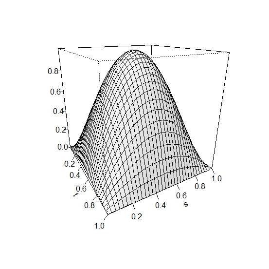
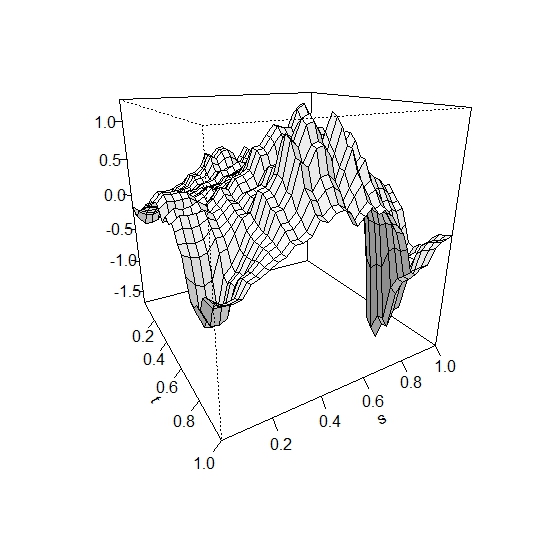
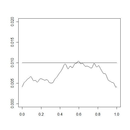
Figure 1: $\beta(t,s)=16s(1-s)t(1-t)$

Figure 2: Using a sample of size $N=30$, we obtain $\hat{\beta}(t,s;2)$ on the left and $\hat{\delta}(t;2)$ with $\delta(t)=.01$ superimposed on the right.

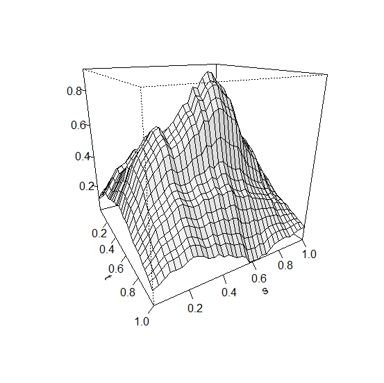
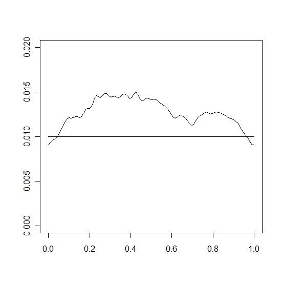
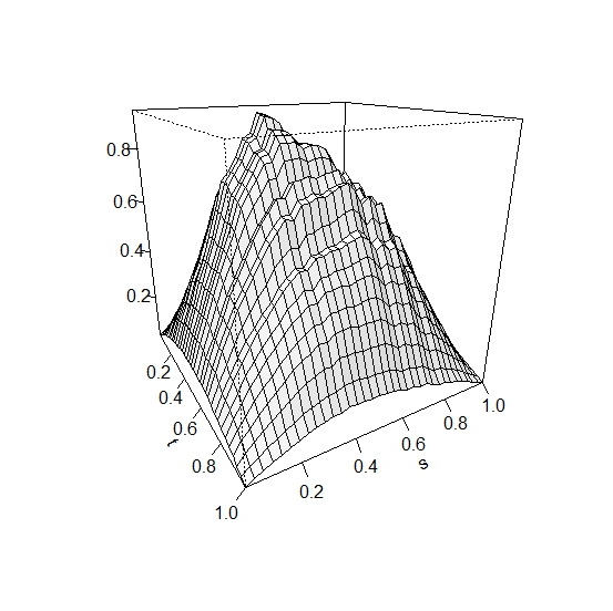
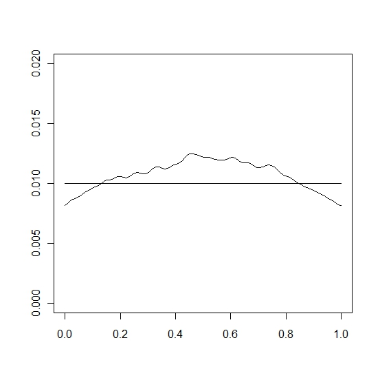
Figure 3: Using a sample of size $N=300$, we obtain $\hat{\beta}(t,s;2)$ on the left and $\hat{\delta}(t;2)$ with $\delta(t)=.01$ superimposed on the right.

Figure 4: Using a sample of size $N=3000$, we obtain $\hat{\beta}(t,s;2)$ on the left and $\hat{\delta}(t;2)$ with $\delta(t)=.01$ superimposed on the right.

4 An example

In this section we show an example illustrating that our model captures the basic features of intraday returns. Let $P_{k}(t)$ denote the price of a stock on day $k$ at time $t$. Then $y_{k}(t)$ can be viewed as the log-returns of the stock, $y_{k}(t)=\log P_{k}(t)-\log P_{k}(t-h)$, during period $h$ (cf. Cyree et al. [10]), where $h$ is typically 1, 5, or 15 minutes. We will use $h=5$ for $5$-minute returns. The volatility of the stock is then represented by $\sigma_{k}^{2}(t)=\mathrm{Var}(y_{k}(t)|\mathcal{F}_{k-1})$.

The first step to simulating the intraday returns is to estimate the parameters, $\delta(t)$ and $\beta(t,s)$, as outlined in Section 3.1. These parameters were estimated for the S&P 100 index based on data from April 1, 1997 to March 30, 2007. The estimated functions, $\hat{\beta}(t,s;2)$ and $\hat{\delta}(t;2)$, are shown in Figure 5.

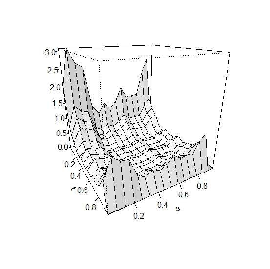
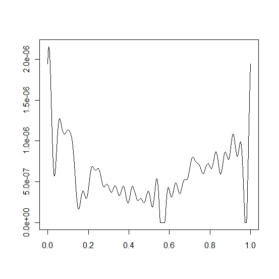
Figure 5: Left: $\hat{\beta}(t,s;2)$ estimated from S&P 100 index. Right: $\hat{\delta}(t;2)$ estimated from S&P 100 index.

Notice in Figure 5 that $\hat{\beta}(t,s;2)$ and $\hat{\delta}(t;2)$ are somewhat larger when $t$ is close to $0$ or $1$. According to (2.2) this suggests that the volatility, $\sigma_{k}^{2}(t)$, tends to be larger at the beginning and end of each trading day. Higher volatilities at the beginning and the end of the trading day have been observed by several authors (cf. Gau [17] and Evans and Speight [15]). This phenomenon is consistent with our observed log-return data based on the S&P 100 index and is captured by our model.

Having estimated the parameters, $\delta(t)$ and $\beta(t,s)$, we can now simulate several days of observations according to (2.1) and (2.2). We will use $\varepsilon_{i}(t)=2^{-200t}\sqrt{\log(2)}W_{i}(2^{400t}/\log(2))$ for the error term, where $W_{i}(t)$ are iid standard Brownian motions. Note that this gives $E(\varepsilon^{2}(t))=1$ for all $t$, which is assumed by our estimation procedure.

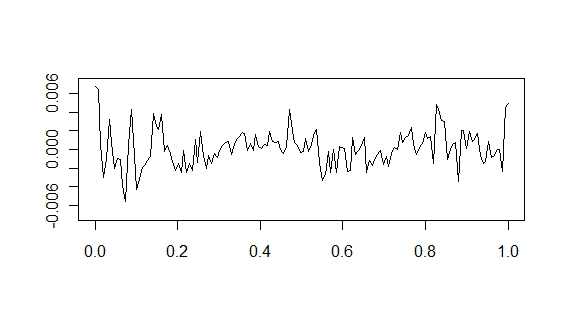
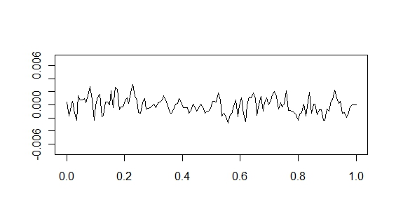
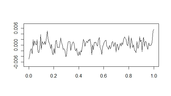
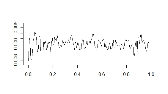
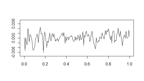
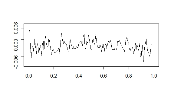
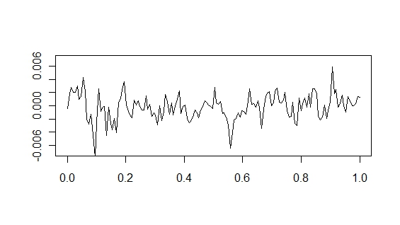
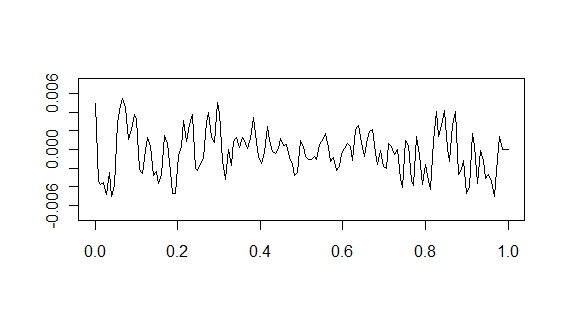
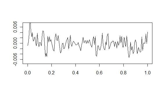
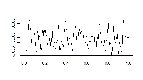
Figure 6: Left panel: Five consecutive days of simulated values for $y_{k}(t)$ . Right panel: 5-minute log-returns for the S&P index between April 11 and April 15, 2000.

We simulated 5 days of log-returns which we compare with the log-returns of the S&P 100 index. The right side of Figure 6 is the plot of the 5-minute returns on the S&P 100 index between April 11 and April 15, 2000. The left side of Figure 6 shows five consecutive days of simulated values for $y_{k}(t)$. The simulations show that our model empirically captures the main characteristics of financial data.

5 Proofs

The proofs of Theorems 2.1 and 2.3 are based on general results for iterated random functions as those in Wu and Shao [27] and Diaconis and Freedman [11]. For the convenience of the reader we shall repeat here the main ideas of [27].

Let $(S,\rho)$ be a complete, separable metric space. Let $\Theta$ be another metric space and let $M:\Theta\times S\to S$ be a measurable function. For a random element $\theta$ with values in $\Theta$, an iterated random function system is defined via the random mappings $M_{\theta}(\cdot)$. More precisely it is assumed that

$$X_{n}=M_{\theta_{n}}(X_{n-1}),\quad n\in\mathbb{N},$$ (5.25)

where $\{\theta_{n},\ -\infty<n<\infty\}$ is an i.i.d. sequence with values in $\Theta$. Thereby it is assumed that $X_{0}$ is independent of $\{\theta_{n},\,n\geq 1\}$. For any $x\in S$ we define

$$S_{n}(x)=M_{\theta_{n}}\circ M_{\theta_{n-1}}\circ\cdots\circ M_{\theta_{1}}(x),\quad n=1,2,\ldots,$$

where $\circ$ denotes the composition of functions. We also introduce the backward version of $S_{n}$, which is given by

$$Z_{n}(x)=M_{\theta_{-1}}\circ M_{\theta_{-2}}\circ\cdots\circ M_{\theta_{-n}}(x),\quad x\in S,\>n=1,2,\ldots.$$

The following theorem is a slight modification of Theorem 2 of [27], so that it is immediately applicable for our purposes.

Theorem 5.1.

(Wu and Shao, 2004.) Assume that
(A) there are $y_{0}\in S$ and $\alpha>0$ such that $E\big{\{}\rho(y_{0},M_{\theta_{0}}(y_{0}))\big{\}}^{\alpha}<\infty$ and
(B) there are $x_{0}\in S$, $\alpha>0$, $0<r_{1}=r_{1}(\alpha)<1$ and $c=c(\alpha)<\infty$ such that

$$E\big{\{}\rho(S_{n}(x),S_{n}(x_{0}))\big{\}}^{\alpha}\leq cr_{1}^{n}\big{\{}\rho(x,x_{0})\big{\}}^{\alpha}$$

for all $x\in S$ and $n\in\mathbb{N}$. Then for all $x\in S$ we have $Z_{n}(x)$ converges almost surely to some $Z_{\infty}$ which is independent of $x$. Furthermore $Z_{\infty}=g(\theta_{0},\theta_{-1},\ldots)$ and

$$E\big{\{}\rho(Z_{n}(x),Z_{\infty})\big{\}}^{\alpha}\leq c_{1}r^{n},$$

where $c_{1}=c_{1}(x,x_{0},y_{0},\alpha)<\infty$ and $0<r=r(\alpha)<1$. Moreover, the process $X_{n}=g(\theta_{n},\theta_{n-1},\ldots)$ is a stationary solution of (5.25). Finally, if we let $X_{0}^{*}=f(\theta_{0}^{\prime},\theta_{-1}^{\prime},\ldots)$ where $\{\theta_{n}^{\prime}\}$ is an independent copy of $\{\theta_{n}\}$, then

$$E\big{\{}\rho(S_{n}(X_{0}^{*}),S_{n}(X_{0}))\big{\}}^{\alpha}\leq c_{2}r_{2}^{n},$$

with some $0<r_{2}=r_{2}(\alpha)<1$ and $c_{2}=c_{2}(\alpha)>0$.

Proof of Theorem 2.1..

We need to show that the conditions of Theorem 5.1 are satisfied when the underlying space is $\mathcal{H}$ with metric $\|\cdot\|_{\mathcal{H}}$ and

$$M_{\theta_{n}}(x)(t)=\delta(t)+\int\beta(t,s)\varepsilon_{n-1}^{2}(s)x(s)ds.$$

To demonstrate (A) of Theorem 5.1 we use $y_{0}(t)=0$, $0\leq t\leq 1$, and get

$$\big{\|}y_{0}-M_{\theta_{0}^{2}}(y_{0})\big{\|}_{\mathcal{H}}^{2}=\int\delta^{2}(t)dt<\infty,$$

by assumption. Since for any $x,x_{0}\in\mathcal{H}$ we have

$$\big{\|}S_{n}(x)-S_{n}(x_{0})\big{\|}_{\mathcal{H}} =\big{\|}M_{\theta_{n}^{2}}(S_{n-1}(x))-M_{\theta_{n}^{2}}(S_{n-1}(x_{0}))\big{\|}_{\mathcal{H}}$$

$$=\bigg{(}\int\bigg{(}\int\beta(t,s)\big{\{}S_{n-1}(x)(s)-S_{n-1}(x_{0})(s)\big{\}}\varepsilon_{n-1}^{2}(s)ds\bigg{)}^{2}dt\bigg{)}^{1/2}$$

$$\leq\bigg{(}\int\bigg{\{}\int\beta^{2}(t,s)\varepsilon_{n-1}^{4}(s)ds\bigg{\}}\int\bigg{\{}S_{n-1}(x)(s)-S_{n-1}(x_{0})(s)\bigg{\}}^{2}dsdt\bigg{)}^{1/2}$$

$$=K(\varepsilon_{n-1}^{2})\,\big{\|}S_{n-1}(x)-S_{n-1}(x_{0})\big{\|}_{\mathcal{H}},$$

by the Cauchy-Schwarz inequality. Repeating the arguments above, we conclude

$$\big{\|}S_{n}(x)-S_{n}(x_{0})\big{\|}_{\mathcal{H}}\leq\big{\|}x-x_{0}\big{\|}_{\mathcal{H}}\prod_{i=0}^{n-1}K(\varepsilon_{i}^{2}).$$

Taking expectations on both sides and using the independence of the $\varepsilon_{i}$ proves (B). ∎

Theorem 2.2 is a simple corollary to Theorem 2.1 and Theorem 5.1. Theorem 2.3 can be proven along the same lines of argumentation and the proof is omitted.

Proof of Propositions 2.1 and 2.2..

First we establish (2.7). We follow the proof of Theorem 2.1. Since $E\big{\{}\|\sigma_{0}^{2}\|_{\mathcal{H}}\big{\}}^{\alpha}=E\big{\{}\|Z_{\infty}\|_{\mathcal{H}}\big{\}}^{\alpha}$, according to the construction in the proof of Theorem 2.1 we have

$$E\big{\{}\|\sigma_{0}^{2}\|_{\mathcal{H}}\big{\}}^{\alpha} =E\big{\{}\|Z_{\infty}\|_{\mathcal{H}}\big{\}}^{\alpha}$$

$$\leq E\big{\{}\|Z_{1}(0)\|_{\mathcal{H}}+\|Z_{1}(0)-Z_{\infty}(0)\|_{\mathcal{H}}\big{\}}^{\alpha}$$

$$\leq 2^{\alpha}\Big{\{}E\big{\{}\|Z_{1}(0)\|_{\mathcal{H}}\big{\}}^{\alpha}+E\big{\{}\|Z_{1}(0)-Z_{\infty}(0)\|_{\mathcal{H}}\big{\}}^{\alpha}\Big{\}},$$

where $0$ denotes the "zero function" on $[0,1]$. According the proof of Theorem 2.1 and Theorem 5.1 the term $E\big{\{}\|Z_{1}(0)-Z_{\infty}(0)\|_{\mathcal{H}}\big{\}}^{\alpha}<\infty$. Furthermore, the term $E\big{\{}\|Z_{1}(0)\|_{\mathcal{H}}\big{\}}^{\alpha}=\Big{(}\int\delta^{2}(t)dt\Big{)}^{\frac{\alpha}{2}}<\infty$. To show (2.10), we note that

$$E\big{\{}\|y_{0}\|_{\mathcal{H}}\big{\}}^{\alpha} =E\bigg{[}\int y_{0}^{2}(t)dt\bigg{]}^{\frac{\alpha}{2}}$$

$$=E\bigg{[}\int\varepsilon_{0}^{2}(t)\sigma_{0}^{2}(t)dt\bigg{]}^{\frac{\alpha}{2}}$$

$$\leq E\big{\{}\|\varepsilon_{0}\|_{\infty}\big{\}}^{\alpha}E\big{\{}\|\sigma_{0}\|_{\mathcal{H}}\big{\}}^{\alpha},$$

since $\varepsilon_{0}$ and $\sigma_{0}$ are independent processes. Proposition 2.1 is proven.

The proof of Proposition 2.2 only requires minor modifications and is therefore omitted. ∎

Proof of Proposition 2.3..

Using recursion 2.1 we have

$$\omega(y_{0},h) =\sup_{0\leq t\leq 1-h}\sup_{0\leq s\leq h}|\varepsilon_{0}(t+s)\sigma_{0}(t+s)-\varepsilon_{0}(t)\sigma_{0}(t)|$$

$$\leq\sup_{0\leq t\leq 1-h}\sup_{0\leq s\leq h}\big{\{}|\varepsilon_{0}(t+s)||\sigma_{0}(t+s)-\sigma_{0}(t)|+|\sigma_{0}(t)||\varepsilon_{0}(t+s)-\varepsilon_{0}(t)|\big{\}}$$

$$\leq\|\varepsilon_{0}\|_{\infty}\omega(\sigma_{0},h)+\|\sigma_{0}\|_{\infty}\omega(\varepsilon_{0},h).$$

The independence of $\varepsilon_{0}$ and $\sigma_{0}$ yields

$$E\big{\{}\|\sigma_{0}\|_{\infty}\omega(\varepsilon_{0},h)\big{\}}^{p}=E\big{\{}\|\sigma_{0}\|_{\infty}\big{\}}^{p}E\big{\{}\omega(\varepsilon_{0},h)\big{\}}^{p}.$$

Proposition 2.2 gives $E\big{\{}\|\sigma_{0}^{2}\|_{\infty}\big{\}}^{p}<\infty$. This implies that $E\big{\{}\|\sigma_{0}\|_{\infty}\big{\}}^{p}<\infty$ and therefore

$$\lim_{h\to 0}E\big{\{}\|\sigma_{0}\|_{\infty}\omega(\varepsilon_{0},h)\big{\}}^{p}=0.$$

The identity $|\sqrt{a}-\sqrt{b}|\leq\sqrt{|a-b|}$, $a,b\geq 0$, implies

$$\omega^{p}(\sigma_{0},h) =\sup_{0\leq t\leq 1-h}\sup_{0\leq s\leq h}|\sigma_{0}(t+s)-\sigma_{0}(t)|^{p}$$

$$\leq\left(\sup_{0\leq t\leq 1-h}\sup_{0\leq s\leq h}|\sigma_{0}^{2}(t+s)-\sigma_{0}^{2}(t)|\right)^{\frac{p}{2}}.$$

Recursion (2.2) gives

$$|\sigma_{0}^{2}(t+s)-\sigma_{0}^{2}(t)| \leq|\delta(t+s)-\delta(t)|+\bigg{|}\int(\beta(t+s,r)-\beta(t,r))y_{-1}^{2}(r)dr\bigg{|}$$

$$\leq\omega(\delta,h)+\sup_{0\leq t\leq 1-h}\sup_{0\leq s\leq h}\sup_{0\leq r\leq 1}|\beta(t+s,r)-\beta(t,r)|\times\int y_{-1}^{2}(r)dr.$$

Hence

$$E\left(\omega^{p}(\sigma_{0},h)\right) =E\big{\{}\sup_{0\leq t\leq 1-h}\sup_{0\leq s\leq h}|\sigma_{0}^{2}(t+s)-\sigma_{0}^{2}(t)|\big{\}}^{\frac{p}{2}}$$

$$\leq 2^{\frac{p}{2}}\Big{\{}\big{[}\sup_{0\leq t\leq 1-h}\sup_{0\leq s\leq h}\sup_{0\leq r\leq 1}|\beta(t+s,r)-\beta(t,r)|\big{]}^{\frac{p}{2}}\times E\big{\{}\|y_{0}\|_{\infty}\}^{p}+\big{[}\omega(\delta,h)\big{]}^{\frac{p}{2}}\Big{\}}.$$

Proposition 2.2 yields that $E\big{\{}\|y_{0}\|_{\infty}\big{\}}^{p}<\infty$ and $E\big{\{}\|\sigma_{0}\|_{\infty}\big{\}}^{p}<\infty$. So by the independence of the processes $\varepsilon_{0}$ and $\sigma_{0}$ we conclude

$$\lim_{h\to 0}\big{\{}\|\varepsilon_{0}\|_{\infty}\omega(\sigma_{0},h)\big{\}}^{p}=0,$$

completing the proof of Proposition 2.3. ∎

Proof of Theorem 3.1.

Under our assumptions it follows from Theorem 2.2 that for any $m\geq 1$

$$E\|Z_{k}-Z_{km}\|_{\mathcal{H}}^{4}\leq\mathrm{const}\times r^{m}$$

where $r\in(0,1)$ and $Z_{km}$ are the $m$–dependent approximations of $Z_{k}$ (constructed by using $\sigma_{km}^{2}$ instead of $\sigma_{k}^{2}$ in the definition of $Z_{k}$). This shows that the notion of $L^{4}$–$m$–approximability suggested in Hörmann and Kokoszka [19] applies to the sequence $\{Z_{k}\}$. As consequence we have with $\hat{c}_{i}=\mathrm{sign}\langle\hat{e}_{i},e_{i}\rangle$ that

$$(a) \quad\max_{1\leq i\leq K}E\|\hat{c}_{i}\hat{e}_{i}-e_{i}\|_{\mathcal{H}}^{2}=O\left(N^{-1}\right);$$

$$(b) \quad\max_{1\leq i\leq K}E|\hat{\lambda}_{i}-\lambda_{i}|^{2}=O\left(N^{-1}\right)$$

and therefore that

$$(a^{\prime}) \quad\max_{1\leq i\leq K}\|\hat{c}_{i}\hat{e}_{i}-e_{i}\|_{\mathcal{H}}=O_{P}\left(N^{-1/2}\right);$$

$$(b^{\prime}) \quad\max_{1\leq i\leq K}|\hat{\lambda}_{i}-\lambda_{i}|=O_{P}\left(N^{-1/2}\right)$$

(See [19, Theorem 3.2].) The random sign $\hat{c}_{i}$ (which we cannot observe) accounts for the fact that $e_{i}$ can be only uniquely identified up to its sign. As our estimator $\hat{\beta}(K)$ doesn’t depend on the signs of the $\hat{e}_{i}$, this poses no problem. We define

$$\sigma_{i,j}=E\langle Z_{1},e_{i}\rangle\langle Z_{2},e_{j}\rangle$$

and let

$$\hat{\sigma}_{i,j}=\frac{1}{N-1}\sum_{k=1}^{N-1}\langle Z_{k},\hat{e}_{i}\rangle\langle Z_{k+1},\hat{e}_{j}\rangle$$

be the empirical counterpart. Then we have

$$E|\sigma_{i,j}-\hat{c}_{i}\hat{c}_{j}\hat{\sigma}_{i,j}| \leq E\left|\frac{1}{N-1}\sum_{k=1}^{N-1}\left(\langle Z_{k},{e}_{i}\rangle\langle Z_{k+1},{e}_{j}\rangle-E\langle Z_{k},{e}_{i}\rangle\langle Z_{k+1},{e}_{j}\rangle\right)\right|$$

$$\quad+E\left|\frac{1}{N-1}\sum_{k=1}^{N-1}\left(\langle Z_{k},\hat{c}_{i}\hat{e}_{i}\rangle\langle Z_{k+1},\hat{c}_{j}\hat{e}_{j}\rangle-\langle Z_{k},{e}_{i}\rangle\langle Z_{k+1},{e}_{j}\rangle\right)\right|$$

$$\quad=:T_{1}(i,j;N)+T_{2}(i,j;N).$$

The processes $\mathcal{Z}_{k}=\mathcal{Z}_{k}(i,j)=\langle Z_{k},{e}_{i}\rangle\langle Z_{k+1},{e}_{j}\rangle$ are strictly stationary for every choice of $i$ and $j$ and we can again define the approximations $\mathcal{Z}_{km}$ in the spirit of Section 2. We have by independence of $\mathcal{Z}_{0}$ and $\mathcal{Z}_{kk}$

$$\sum_{h\geq 0}|\mathrm{Cov}(\mathcal{Z}_{0},\mathcal{Z}_{h})| \leq E\mathcal{Z}_{0}^{2}+\left(E\mathcal{Z}_{0}^{2}\right)^{1/2}\times\sum_{h\geq 1}\left(E(\mathcal{Z}_{h}-\mathcal{Z}_{hh})^{2}\right)^{1/2}$$

$$\leq E\|Z_{0}\|_{\mathcal{H}}^{4}+E\|Z_{0}\|_{\mathcal{H}}^{2}\times\sum_{h\geq 1}\left(E(\mathcal{Z}_{h}-\mathcal{Z}_{hh})^{2}\right)^{1/2}.$$

Further we have by repeated application of the Cauchy-Schwarz inequality that

$$E(\mathcal{Z}_{h}-\mathcal{Z}_{hh})^{2} =E\left[\langle Z_{h},e_{i}\rangle\langle Z_{h+1},e_{j}\rangle-\langle Z_{hh},e_{i}\rangle\langle Z_{h+1,h},e_{j}\rangle\right]^{2}$$

$$\quad\leq 2\left\{E\left[\langle Z_{h}-Z_{hh},e_{i}\rangle\langle Z_{h+1},e_{j}\rangle\right]^{2}+E\left[\langle Z_{hh},e_{i}\rangle\langle Z_{h+1}-Z_{h+1,h},e_{j}\rangle\right]^{2}\right\}$$

$$\quad\leq 2\left\{E\langle Z_{h}-Z_{hh},e_{i}\rangle^{2}E\langle Z_{h},e_{j}\rangle^{2}+E\langle Z_{hh},e_{i}\rangle^{2}E\langle Z_{h+1}-Z_{h+1,h},e_{j}\rangle^{2}\right\}$$

$$\quad\leq 2E\|Z_{0}\|^{2}_{\mathcal{H}}\left\{E\|Z_{h}-Z_{hh}\|_{\mathcal{H}}^{2}+E\|Z_{h+1}-Z_{h+1,h}\|_{\mathcal{H}}^{2}\right\}$$

$$\quad\leq\mathrm{const}\times r^{h},$$

for some $r\in(0,1)$. This proves that the autocovariances of the process $\{\mathcal{Z}_{k}\}$ are absolutely summable. A well known result in time series analysis thus implies that

$$(N-1)\mathrm{Var}\left(\frac{1}{N-1}\sum_{k=1}^{N-1}\mathcal{Z}_{k}\right)\leq 2\sum_{h\geq 0}|\mathrm{Cov}(\mathcal{Z}_{0},\mathcal{Z}_{h})|\leq c_{0},\quad\forall N\geq 2,$$

(see e.g. the proof of Theorem 7.1.1. in Brockwell and Davis [8]) where, as we have shown, the constant $c_{0}$ is independent of the choice of $i$ and $j$ in the definition of $\mathcal{Z}_{k}$. Hence $\max_{1\leq i,j\leq K}T_{1}(i,j;N)=O_{P}\left(N^{-1/2}\right)$.

Using relation ($a$) above, one can show that also $\max_{1\leq i,j\leq K}T_{2}(i,j;N)=O_{P}\left(N^{-1/2}\right)$. We thus have

$$(c)\quad\max_{1\leq i,j\leq K}|\sigma_{i,j}-\hat{c}_{i}\hat{c}_{j}\hat{\sigma}_{i,j}|=O_{P}\left(N^{-1/2}\right).$$

We have now the necessary tools to prove Theorem 3.1. By relations ($a^{\prime}$), ($b^{\prime}$) and ($c$) we have that

$$\left\|\beta(K)-\hat{\beta}(K)\right\|_{\mathcal{S}}=\left\|\sum_{1\leq i,j\leq K}\left(\frac{\sigma_{j,i}}{\lambda_{j}}e_{j}\otimes e_{i}-\frac{\hat{\sigma}_{j,i}}{\hat{\lambda}_{j}}\hat{e}_{j}\otimes\hat{e}_{i}\right)\right\|_{\mathcal{S}}$$

$$\quad\leq\sum_{1\leq i,j\leq K}\left\{\left|\frac{\sigma_{j,i}}{\lambda_{j}}-\frac{\hat{c}_{j}\hat{c}_{i}\hat{\sigma}_{j,i}}{\hat{\lambda}_{j}}\right|+\left|\frac{\sigma_{j,i}}{\hat{\lambda}_{j}}\right|\left\|e_{j}\otimes e_{i}-\hat{c}_{j}\hat{e}_{j}\otimes\hat{c}_{i}\hat{e}_{i}\right\|_{\mathcal{S}}\right\}$$

$$\quad\leq K^{2}\left\{O_{P}\left(N^{-1/2}\right)+O_{P}(1)\max_{1\leq i,j\leq K}\left\|e_{j}\otimes e_{i}-\hat{c}_{j}\hat{e}_{j}\otimes\hat{c}_{i}\hat{e}_{i}\right\|_{\mathcal{S}}\right\}.$$

The proof follows from $\left\|e_{j}\otimes e_{i}-\hat{c}_{j}\hat{e}_{j}\otimes\hat{c}_{i}\hat{e}_{i}\right\|_{\mathcal{S}}\leq\|\hat{c}_{j}\hat{e}_{j}-e_{j}\|_{\mathcal{H}}+\|\hat{c}_{i}\hat{e}_{i}-e_{i}\|_{\mathcal{H}}.$ ∎

References

- [1] Angelidis, T. and Degiannakis, S. (2008). Volatility forecasting: Intra-day versus inter-day models. Journal of International Financial Markets, Institutions & Money, 18, 449-465.
- [2] Aue, A., Hörmann, S., Horváth, L., Hǔsková, M., and Steinebach, J. (2010+). Sequential testing for the stability of high frequencey portfolio betas. Preprint.
- [3] Barndorff-Nielsen, O.E., Hansen, P.R., Lunde, A. and Shephard, N. (2008). Designing realised kernels to measure the ex-post variation of equity prices in the presence of noise. Econometrica 76, 1481–1536.
- [4] Barndorff-Nielsen, O.E. and Shephard, N. (2004). Econometric analysis of realized covariation: High frequency based covariance, regression, and correlation in financial economics. Econometrica 72, 885–925.
- [5] Bollerslev, T. (1990). Modeling the coherence in short-run nominal exchange rates: multivariate generalized ARCH model. Review of Economics and Statistics, 74, 498–505.
- [6] Bosq, D. (2000). Linear Processes in Function Spaces. Springer, New York.
- [7] Bougerol, P. and Picard, N. (1992). Stationarity of GARCH processes and of some nonnegative time series. Journal of Econometrics, 52, 115–127.
- [8] Brockwell, P. J. and Davis, R. A. (1991). Time Series: Theory and Methods Springer.
- [9] Cardot, H., Ferraty, F. and Sarda, P. (1999). Functional linear model. Statistics & Probability Letters 45, 11-22.
- [10] Cyree, K. K., Griffiths, M. D. and Winters, D. B. (2004). An empirical examination of intraday volatility in euro-dollar rates. The Quaterly Review of Economics and Finance, 44, 44-57.
- [11] Diaconis, P. and Freedman, D. (1999). Iterated random functions. Siam Review, 41, 45–76.
- [12] Didericksen, D. and Kokoszka, P. and Zhang, X. (2010). Empirical properties of forecasts with the functional autoregressive model. Technical Report, Utah State University.
- [13] Elezović, S. (2009). Functional modelling of volatility in the Swedish limit order book. Computational Statistics & Data Analysis, 53, 2107-2118.
- [14] Engle, R. F. (1982). Autoregressive conditional heteroskedasticity with estimates of the variance of United Kingdom inflation. Econometrica, 50, 987–1007.
- [15] Evans, K. P. and Speight, A. E. H. (2010). Intraday periodicity, calendar and announcement effects in Euro exchange rate volatility. Research in International Business and Finance, 24, 82-101.
- [16] Fatum, R. and Pedersen, J. (2009). Real-time effects of central bank intervention in the euro market. Journal of International Economics, 78, 11-20.
- [17] Gau, Y-F. (2005). Intraday volatility in the Taipei FX market. Pacific-Basin Finance Journal, 13, 471-487.
- [18] Harrison, J.M., Pitbladdo, R. and Schaefer, S.M. (1984). Continuous prices in frictionless markets have infinite variation. Journal of Business,57, 353–365.
- [19] Hörmann, S. and Kokoszka, P. (2010). Weakly dependent functional data. The Annals of Statistics, 38, 1845–1884.
- [20] Jacod, J., Li, Y., Mykland, P.A., Podolskij, M. and Vetter, M. (2009). Microstructure noise in the continuous case: the pre-averaging approach. Stochastic Processes and their Applications 119, 2249–2276.
- [21] Jeantheau, T. (1998). Strong consistency of estimators for multivariate ARCH models. Econometric Theory, 14, 70–86.
- [22] Ling, S. and McAleer, M. (2002). Necessary and sufficient moment conditions for the GARCH(p,q) and asymmetric power GARCH(p,q) models. Econometric Theory 18, 722-729.
- [23] Nelson, D. B. (1990). Stationarity and persistence in the GARCH () model. Econometric Theory, 6, 318–334.
- [24] Polyanin, A. and Manzhirov, A. (1998). Handbook of Integral Equations CRC Press, London.
- [25] Silvennoinen, A. and Teräsvirta, T. (2009). Multivariate GARCH models. In: Handbook of Financial Time Series (Eds: T.G. Anderson et al.) pp. 201-229. Springer-Verlag, New York.
- [26] Stout, W.F. (1974). Almost Sure Convergence. Acadamemic Press, New York.
- [27] Wu, W. and Shao, X. (2004). Limit theorems for iterated random functions. Journal of Applied Probability, 41, 425–436.
- [28] Zhang, L., Mykland, P.A. and Aït-Sahalia, Y. (2005). A tale of two time scales: determining integrated volatility with noisy high-frequency data. Journal of the American Statistical Association 100, 1394–1411.