Abstract

We characterize the completely positive trace-preserving maps on qutrits, (qutrit channels) according to their covariance and symmetry properties. Both discrete and continuous groups are considered. It is shown how each symmetry group, restricts arbitrariness in the parameters of the channel to a very small set. Although the explicit examples are related to qutrit channels, the formalism is sufficiently general to be applied to qudit channels.

Keywords: Quantum channels, covariant channels, symmetry.
PACS Numbers: $03.67$.-a, $03.65$.Aa, $03.67$.Hk

1 Introduction

The problem of characterization of quantum channels is one of the interesting and important problems of quantum information science. On the physical side, a quantum channel is the most general physical process that a quantum system can undergo [1, 2], when initially it is only classically correlated [3] with its environment. (Non-positivity of the corresponding map indicates the presence of an initial quantum correlation between the system and the environment [3]). On the mathematical side, this problem is equivalent to characterizing completely positive maps. One of the basic results is that, any channel has an operator sum representation, that is, for any such channel ${\cal E}$ can be represented as

$${\cal E}(\rho)=\sum_{k}A_{k}\rho A_{k}^{\dagger},$$ (1)

where the condition $\sum_{k}A_{k}^{\dagger}A_{k}=I$ guarantees that the channel is trace preserving. What renders the characterization of such channels difficult, is due to the non-uniqueness of the kraus representation. That is any channel can have infinitely many equivalent Kraus representation. Any two such representations, one by the Kraus set $\{A_{a}\}$, and the other by $\{B_{a}\}$ are related by a unitary transformation [4], that is, there is a unitary matrix $\Omega$ such that

$$B_{a}=\sum_{b}\Omega_{ab}A_{b}.$$ (2)

Despite this difficulty, a complete characterization of qubit channels is at hand thanks to the works of [5] and [6]. We now know that any qubit channel is of the following form

$${\cal E}(\rho)=U{\cal E}_{{\bf t},\Lambda}(V\rho V^{-1})U^{-1},$$ (3)

where ${\cal E}_{{\bf t},\Lambda}(\rho)$ maps the vectors in the Bloch sphere as follows ${\bf r}\longrightarrow{\bf r^{\prime}}={\bf{\Lambda}}{\bf r}+{\bf t}$, where ${\bf t}$ is a three-dimensional vector, $\Lambda=diag(\lambda_{1},\lambda_{2},\lambda_{3})$ and the vector $\overrightarrow{\lambda}=(\lambda_{1},\lambda_{2},\lambda_{3})$ is contained in a tetrahedron spanned by the four corners of the unit cube with $\lambda_{1}\lambda_{2}\lambda_{3}=1$ [6, 7]. For higher dimensional channels no such characterization has yet been made, even for the simplest case of qutrit channels. The difficulty with higher dimensional channels, lies with both the large number of parameters needed for description of states and with the absence of a proper geometrical representation for states, as Bloch sphere for qubits. In fact the positivity of the density matrix for qudits does not lead to simple conditions and simple geometry [8, 9, 10, 11, 12].

To see the root of the problem for characterization of higher dimensional channels, let us take the simplest example of $d=3$. A qutrit state can be described by a matrix $\rho=\frac{1}{3}(I+{\sqrt{3}}{\bf r}\cdot{\bf\Gamma})$, where $\Gamma_{1}$ to $\Gamma_{8}$ are the Gell-Mann matrices (a Hermitian basis for the Lie algebra of $su(3)$), and ${\bf r}$ is an 8-dimensional vector with ${\bf r}\cdot{\bf r}\leq 1$. Therefore the role of the two-dimensional Bloch sphere is played by a 7 dimensional sphere, however the point and the root of difficulty is that not all the vectors inside this sphere represent physical states, i.e. positive states $\rho$. In general any completely positive map induces an affine transformation on the vector ${\bf r}$ in the form ${\bf r}\longrightarrow{\bf r^{\prime}}={\bf\Lambda}{\bf r}+{\bf t}$. For qubits, local unitary changes of basis for the input and output spaces, diagonalize the matrix $\Lambda$, hence lead to the form (3), however for qutrits, the parameters of these local unitaries ($SU(3)\otimes SU(3)$) are much less than those of ${\bf\Lambda}$ (which is equal to $8^{2}$) and this diagonalization is not possible. This renders a complete characterization of qutrit channels difficult.

Nevertheless, the problem of characterizing qutrit maps, has been tackled from different points of view. In [13], a special class of qutrit channels whose matrix $\Lambda$ of affine transformation is already diagonal has been studied to find the complete positivity constraints on qutrit channels. In [14], general properties of the affine map on polarization vectors, obtained from completely positive maps on d-level states (qudits) ,has been obtained. In particular special classes of qudit channels with special class of Kraus operators, i.e. unitary, Hermitian, and orthogonal, have been investigated.

In this work, we follow a different approach to categorize qutrit channels in terms of their covariance or symmetry property under some discrete or continuous symmetry group. Our study like the ones in [5] and [6] does not provide an exhaustive characterization of qutrit channels, but provides a framework for a better understanding of the space of qutrit channels. This study sheds light on some aspects of these channels which we hope along with other studies will pave the way for a full characterization of these channels in the future.

The structure of this paper is as follows: In section (2), we provide the preliminary notations about completely positive channels and set up our notations and conventions. In sections (3) and (4), we explain the concept of covariance and symmetry of quantum channels and derive the conditions that these properties impose on the Kraus operators of such channels. In sections (5) and (6) we study in detail several classes of examples, both for discrete and for continuous groups. Although we mainly study the qutrit channels, the formalism that we explain and indeed some of the examples we suggest are general and apply for quantum channels on d-dimensional states or qudits.

2 Preliminaries

The vector space of $d$ dimensional complex square matrices is denoted by $M_{d}$. With the definition of the Hilbert-Schmidt inner product $\langle A,B\rangle=tr(A^{\dagger}B)$ it becomes a Hilbert space of dimension $d^{2}$. Let ${\ \Gamma_{\mu}\ (\mu=0,\cdots,d^{2}-1})$ be an orthonormal hermitian basis for this vector space

$$\langle\Gamma_{\mu},\Gamma_{\nu}\rangle=tr(\Gamma_{\mu}^{\dagger}\Gamma_{\nu})=\delta_{\mu,\nu}.$$ (4)

Any unit-trace matrix $\rho\in M_{d}$ can be expanded as

$$\rho=\sum_{\mu=0}^{d^{2}-1}\rho_{\mu}\Gamma_{\mu}=\frac{1}{d}I+\sum_{i=1}^{d^{2}-1}\rho_{i}\Gamma_{i},$$ (5)

where

$$\rho_{\mu}=\langle\Gamma_{\mu},\rho\rangle=tr(\Gamma_{\mu}^{\dagger}\rho),$$ (6)

and for the first component we have

$$\Gamma_{0}=\frac{1}{\sqrt{d}}I,\hskip 28.45274pt\rho_{0}=\frac{1}{\sqrt{d}}.$$ (7)

This, together with (4) implies that the matrices $\Gamma_{i}$ are traceless. Note that we use the Latin indices $i,j,\cdots$ for $\mu\neq 0$. For a density matrix, the condition $tr(\rho^{2})\leq 1$, constrains the polarization vector to lie within a sphere of radius $\sqrt{1-\frac{1}{d}}$. However not all the vectors in this sphere represent density matrices, due to the extra condition of the positivity of the density matrix [9].

A completely positive map ${\cal E}:M_{d}\longrightarrow M_{d}$, i.e. a channel is represented as

$$\rho^{\prime}={\cal E}(\rho)=\sum_{a}A_{a}\rho A_{a}^{\dagger},$$ (8)

where the set of operators $\{{\cal A}_{a}\}$ are called Kraus operators [2]. It is well-known that any two Kraus representations of a channel are connected by a unitary transformation [4], that is if $\{A_{a}\}$ and $\{B_{a}\}$ are Kraus operators of the same channel ${\cal E}$, then there exists a unitary matrix $\Omega$ such that

$$A_{a}=\sum_{b}\Omega_{ab}B_{b}.$$ (9)

In writing this transformation, one assumes that the two sets of Kraus operators are of equal size, since one can always add zero Kraus operators without changing the channel.

To find how the polarization vector transforms under such a map, we note that

$${\cal E}(\rho)=\sum_{\mu}\rho^{\prime}_{\mu}\Gamma_{\mu}=\sum_{a,\nu}\rho_{\nu}A_{a}\Gamma_{\nu}A_{a}^{\dagger},$$ (10)

from which we obtain

$$\rho^{\prime}_{\mu}=\Lambda_{\mu,\nu}\rho_{\nu},$$ (11)

in which

$$\Lambda_{\mu,\nu}=\langle\Gamma_{\mu},{\cal E}(\Gamma_{\nu})\rangle=\sum_{a}tr(\Gamma_{\mu}^{\dagger}A_{a}\Gamma_{\nu}A_{a}^{\dagger}).$$ (12)

For a trace-preserving map ($tr({\cal E}(\rho)=tr(\rho)$), we have $\sum_{a}A_{a}^{\dagger}A_{a}=I$ and for a unital (${\cal E}(I)=I$), we have $\sum_{a}A_{a}A_{a}^{\dagger}=I$. Therefore using (12), we find

$$\Lambda_{0i}=0\hskip 28.45274pt{\rm if\ \ {\cal E}\ \ is\ trace-preserving\ },$$ (13)

$$\Lambda_{i0}=0\hskip 28.45274pt{\rm if\ \ {\cal E}\ \ is\ unital\ }.$$ (14)

In both cases, we always have $\Lambda_{00}=1$. For trace-preserving maps the form of the matrix $\Lambda$ becomes

$$\left(\begin{array}[]{c}\frac{1}{\sqrt{d}}\\ {\bf\rho^{\prime}}\end{array}\right)=\left(\begin{array}[]{cc}1&0\\ {\bf T}&{\bf\Lambda}\end{array}\right)\left(\begin{array}[]{c}\frac{1}{\sqrt{d}}\\ {\bf\rho}\end{array}\right),$$ (15)

which means the action of the channel on the vector ${\bf\rho}:=(\rho_{1},\cdots\rho_{d^{2}-1})$ is an affine map, i.e. ${\rho}\longrightarrow{\bf\Lambda}{\bf\rho}+{\bf T}$. An analysis of the completely positive maps based on these affine maps, with examples of qutrit channels has been carried out in [14].

As pointed out in the introduction, we want to study qutrit channels from the perspective of their covariance and symmetry properties. To this end, we begin the next section with general remarks on covariance of completely positive maps.

3 Covariant Channels

Let $G$ be a group with $D^{{}^{(1)}}$ and $D^{{}^{(2)}}$ being its representations on $M_{d}$. We call the channel ${\cal E}$ covariant under group $G$ with respect to these two representations if for all $g\in G$, the following relation holds

$$D^{{}^{(2)}}(g){\cal E}(\rho)D^{{}^{(2)}}(g^{-1})={\cal E}(D^{{}^{(1)}}(g)\rho D^{{}^{(1)}}(g^{-1})).$$ (16)

This means that a transformation of the input density matrix by $D^{{}^{(1)}}(g)$ results in a corresponding transformation of the output density matrix by $D^{{}^{(2)}}(g)$. Note that although the input and output density matrices may be of the same dimensions, they may transform according to different representations of the symmetry group. We will see examples in section (6.3), when we discuss channels covariant under the $Su(3)$ group which has two inequivalent 3-dimensional representations.

Besides this appealing property, such channels offer a lot of convenience, when we want to calculate their one-shot classical capacities $C^{1}({\cal E})$ [15]. To see this, we note

$$C^{1}({\cal E})=Sup_{\{p_{i},\rho_{i}\}}\chi({\cal E},\{p_{i},\rho_{i}\})=Sup_{\{p_{i},\rho_{i}\}}\left[S(\sum_{i}p_{i}{\cal E}(\rho_{i}))-\sum_{i}p_{i}S({\cal E}(\rho_{i}))\right].$$ (17)

Here, $\chi$ and $S$ denote respectively the Holevo quantity and the von Newmann entropy, and the maximization is performed over all input ensembles $\{p_{i},\rho_{i}\}$. For a covariant channel, with irreducible representation $D^{{}^{(2)}}$, the problem of finding an optimal ensemble reduces to the problem of finding the minimum output entropy state $\rho^{*}:=|\psi^{*}\rangle\langle\psi^{*}|$, i.e. the pure state which minimizes the second term $S({\cal E}(\rho^{*}))$ [16, 17]. (Purity of this state follows from the convexity of the output entropy) Once this state is found, we can maximize the first term and hence the Holevo quantity itself by taking as the input ensemble the uniformly distributed ensemble of $\rho(g)=D^{{}^{(1)}}(g)\rho^{*}D^{{}^{(1)}}(g^{-1})$. In case that $D^{{}^{(2)}}$ is an irreducible representation, one finds that [18]

$$\frac{1}{|G|}\sum_{g\in G}D^{{}^{(2)}}(g){\cal E}(\rho^{*})D^{{}^{(2)}}(g^{-1})=\frac{1}{d}I,$$ (18)

which means that the first term will take its maximum value for such an ensemble. Therefore the one-shot classical capacity of covariant channels will be found to be

$$C({\cal E})=\log_{2}d-S({\cal E}(\rho^{*})).$$ (19)

Here we see how covariant property of the channel reduces a problem which involved an optimization over a large parameter space (in this case the space of input ensembles) to the much simpler problem of finding the minimum output entropy of the channel. The input space that we have to search for can be further reduced if the channel has some kind of symmetry, like

$${\cal E}(\rho)={\cal E}(h\rho h^{-1}),$$

where $h$ is an element of a group $H$ . In such a case it is enough to search over a subset of states which are invariant under $H$. Furthermore, due to the convexity of the output entropy, the search can be restricted to be over pure states with that symmetry.

Before going to a systematic discussion for constructing covariant maps, let us note the simplest examples. Clearly the identity channel ${\cal E}_{I}(\rho)=\rho$, is a CPT map which is covariant under any group of transformations, with $D^{(1)}=D^{(2)}.$ The completely mixing CPT map ${\cal E}_{0}(\rho)=\frac{1}{d}tr(\rho)I$ is covariant under any transformation group with arbitrary representations $D^{(1)}$ and $D^{(2)}$. As a less trivial example, consider the map ${\cal E}_{T}(\rho)=\frac{1}{d+1}(tr(\rho)I+\rho^{T})$, where $\rho^{T}$ denotes the transpose of $\rho$. Although transposition by itself is not a completely positive map, the above convex combination with the mixing map is a CPT, since it has a Kraus representation in the form:

$${\cal E}_{T}(\rho)=\frac{1}{2(d+1)}\sum_{i,j}A_{ij}\rho A_{i,j}^{\dagger},$$ (20)

where $A_{ij}=|i\rangle\langle j|+|j\rangle\langle i|.$ This channel is covariant under any group where $D^{(1)}(g)=g$ and $D^{(2)}(g)=g^{*}$. The convex combination of any two channels which are covariant under the same representations of a given group, is also covariant under the same group with the same representations. For example consider a qudit channel. Considering the qudit as the state of a spin-$(d-1)/2$ particle, the group $SO(d)$ has a natural action on it in the form of rotation $|\psi\rangle\longrightarrow R|\psi\rangle$, or $\rho\longrightarrow R\rho R^{T}$. Noting that the representation $R$ is real, $R=R^{*}$, we find that the following qudit channel is covariant under the rotation group $SO(d)$:

$${\cal E}(\rho)=a{\cal E}_{I}(\rho)+b{\cal E}_{0}(\rho)+(1-a-b){\cal E}_{T}(\rho),$$ (21)

or by redefining the parameters,

$${\cal E}(\rho)=\alpha\ tr(\rho)\ I+\beta\ \rho+\gamma\ \rho^{T},$$ (22)

with $\alpha d+\beta+\gamma=1.$

In order to characterize covariant channels in a systematic way, it is best to consider the Kraus representation of such channels in terms of which, equation (16) reads

$$D^{{}^{(2)}}(g)\sum_{a}A_{a}\rho A_{a}^{\dagger}D^{{}^{(2)}}(g^{-1})=\sum_{a}A_{a}(D^{{}^{(1)}}(g)\rho D^{{}^{(1)}}(g^{-1}))A_{a}^{\dagger},$$ (23)

or equivalently

$$\sum_{a}A_{a}\rho A_{a}^{\dagger}=\sum_{a}D^{{}^{(2)}}(g^{-1})A_{a}(D^{{}^{(1)}}(g)\rho D^{{}^{(1)}}(g^{-1}))A_{a}^{\dagger}D^{{}^{(2)}}(g).$$ (24)

However according to (9) any two different Kraus representations of a channels are necessarily related by a unitary transformation, which implies that

$$D^{{}^{(2)}}(g^{-1})A_{a}D^{{}^{(1)}}(g)=\sum_{b}\Omega_{ab}(g)A_{b}.$$ (25)

Repeating this relation for two different group elements $g$ and $g^{\prime}$ and combining the two we find that

$$\sum_{b}\Omega_{ab}(g)\Omega_{bc}(g^{\prime})=\Omega_{ac}(gg^{\prime}),$$

which means that $\Omega$ is a unitary representation of the group $G$. The dimension of this representation is the same as the number of Kraus operators. Moreover from (25) one finds that

$$D^{{}^{(1)}}(g^{-1})A_{a}^{\dagger}D^{{}^{(2)}}(g)=\sum_{b}\Omega^{*}_{ab}(g)A_{b}^{\dagger}.$$ (26)

Combining this relation with (25), we find that

$$[D^{{}^{(1)}}(g),\sum_{a}A_{a}^{\dagger}A_{a}]=0,$$ (27)

$$[D^{{}^{(2)}}(g),\sum_{a}A_{a}A_{a}^{\dagger}]=0.$$ (28)

The first relation implies that if $D^{{}^{(1)}}$ is an irreducible representation, then according to the Schur’s Lemma [18], $\sum_{a}A_{a}^{\dagger}A_{a}\propto I$ and hence by appropriate normalization, the map ${\cal E}$ can be made trace-preserving. Similarly the second relation implies that if $D^{{}^{(2)}}$ is an irreducible representation, $\sum_{a}A_{a}A_{a}^{\dagger}$ $\propto I$ and hence by appropriate normalization, the channel ${\cal E}$ can be made unital.

To find channels with covariant property we should find a set of Kruas operators satisfying equation (25), where $D^{{}^{(1)}}$, $D^{{}^{(2)}}$ and $\Omega$ are the representations of the group. There are many different choices for the representations of a group, but they may give the same or equivalent maps. By the following remarks we introduce the strategy by which we can restrict our attention to limited number of representations for $D^{{}^{(2)}}$, $D^{{}^{(1)}}$ and $\Omega$.

Remark 1: For $\Omega$ it is enough to consider all the irreducible representations of the group. For each irreducible representation $\Omega^{(i)}$ we can find a set of Kraus operators satisfying

$$D^{{}^{(2)}}(g^{-1})A^{(i)}_{a}D^{{}^{(1)}}(g)={\Omega}^{(i)}_{ab}(g)A^{(i)}_{b},\hskip 28.45274pt$$ (29)

where ${\Omega}^{(i)}$ is an irreducible representation of $G$ ($i=1\cdots K$, labels the $K$ different irreducible representation of $G$). Therefore we can define $K$ sets of Kraus operators or equivalently $K$ channels which are covariant under $G$

$${\cal E}^{(i)}(\rho)=\sum_{a}A^{(i)}_{a}\rho A^{(i)^{\dagger}}_{a}.$$ (30)

It is clear that any convex combination of these maps is also covariant under the action of the group $G$. Therefore the overall solution can be represented by

$${\cal E}=\sum_{i=1}^{K}\lambda_{i}{\cal E}^{(i)},$$ (31)

and it is enough to consider irreducible representations of $\Omega$ without loss of generality. Note that the representations which we choose for $D^{{}^{(1)}}$ and $D^{{}^{(2)}}$ need not be irreducible. In fact we will see explicit cases of reducible representations in the examples which follow the general formalism.

Remark 2: Let the representations $D^{{}^{(1)}}$ and $D^{{}^{(2)}}$ be respectively equivalent to the representations $D^{\prime}_{1}$ and $D^{\prime}_{2}$, i.e. let $U$ and $V$ be unitary operators acting on $M_{d}$ such that for all $g\in G$

$$D^{\prime}_{1}(g)=UD^{{}^{(1)}}(g)U^{\dagger},\hskip 28.45274ptD^{\prime}_{2}(g)=VD^{{}^{(2)}}(g)V^{\dagger},$$

If the channel ${\cal E}$ is covariant with respect to $D^{{}^{(1)}}$ and $D^{{}^{(2)}}$, the channel ${\cal E^{\prime}}:=V\circ{\cal E}\circ U$ will be covariant with respect to $D^{\prime}_{1}$, and $D^{\prime}_{2}$. The channel ${\cal E}^{\prime}$ is defined as

$${\cal E}^{\prime}(\rho)=V{\cal E}(U\rho U^{-1})V^{-1}.$$ (32)

Therefore without loss of generality we consider only non-equivalent representations for $D^{{}^{(1)}}$ and $D^{{}^{(2)}}$.

Before embarking into an investigation of such maps for qutrit channels, we first study in general another important property, namely symmetry of a channel under a group of transformation.

4 Symmetric Maps

A symmetric channel has the property that for elements $g\in G$ of a group the following property holds

$${\cal E}(D(g)\rho D(g^{-1}))={\cal E}(\rho).$$ (33)

In this case, we say that ${\cal E}$ is symmetric with respect to the representation $D$ of the group. An example of such a channel is the bit-flip channel, ${\cal E}(\rho)=(1-p)\rho+p\ X\rho X$, with $p=\frac{1}{2}$ which is symmetry under the group $G=\{I,X\},$ where $X$ is the bit-flip operator.

In terms of the Kraus representations, this is equivalent to

$$\sum_{a}A_{a}D(g)\rho D(g^{-1})A_{a}^{\dagger}=\sum_{a}A_{a}\rho A_{a}^{\dagger},$$ (34)

or according to (9)

$$A_{a}D(g)=\sum_{b}\Omega_{ab}(g)A_{b},$$ (35)

where again $\Omega$ is a representation of $G$. Obviously if the channel ${\cal E}$ is symmetric with respect to the representation $D$, then the channel ${\cal E}\circ{\cal U}$ will be symmetric with respect to the equivalent representation $D^{\prime}=UDU^{-1}$ . Therefore we only need to consider the completely positive maps which are symmetric under inequivalent representations of a given group.

In the next sections we investigate in more detail examples of completely positive maps which are covariant or symmetric under various discrete or continuous groups, with an emphasis on qutrit channels. We split the examples into two separate parts and consider first the discrete groups and then the continuous groups.

5 Examples of covariant qutrit channels under discrete groups

In this section we consider several discrete groups and find classes of channels which are covariant and/or symmetric with respect to different representations of these groups. First we consider a cyclic group and then proceed to other Abelian and Non-Abelian discrete groups.

5.1 The Abelian case: Cyclic groups

Consider a cyclic group of order $n$ which is generated by a single operator called $X$, where $X^{n}=I$. The order of the group is generally has nothing to do with the dimension of the Hilbert space, for example $X$ can be the operator which flips the basis states $|1\rangle$ and $|2\rangle$ without affecting the basis state $|0\rangle$ in which case $n=2$, or it can shift all the basis states by one unit, i.e. $X|i\rangle=|i+1,\ {\rm mod\ d}\rangle$ in which case $n=d$. Being Abelian, we know that all the irreducible representations of this group are one dimensional [18]. Each such representation is labeled by one integer $k\in\{0,1,\cdots n-1\}$. According to (29), for $\Omega$ we need only take one such representation where $X$ is represented by $e^{\frac{2\pi ik}{n}}$. We have to solve the following equation for the single Kraus operator $A^{(k)}$

$$D^{{}^{(2)}}(X^{-1})A^{(k)}D^{{}^{(1)}}(X)=e^{\frac{2\pi ik}{n}}A^{(k)}.$$ (36)

To solve this equation we use the eigenvectors of the operators $D^{{}^{(1)}}(X)$ and $D^{{}^{(2)}}(X)$. Let

$$D^{{}^{(1)}}(X)|\xi_{r}\rangle=e^{\frac{2\pi ir}{n}}|\xi_{r}\rangle$$ (37)

and

$$D^{{}^{(2)}}(X)|\eta_{s}\rangle=e^{\frac{2\pi is}{n}}|\eta_{s}\rangle,$$ (38)

then the general solution of (36) will be given by

$$A^{(k)}:=\sum_{l}a_{l,l+k}|\eta_{l}\rangle\langle\xi_{l+k}|.$$ (39)

A map whose Kraus operators are of the above form, will be covariant with respect to the given cyclic group. To make such a map trace-preserving, the condition $\sum_{k}{A^{(k)}}^{\dagger}A^{(k)}$ is imposed which in view of the explicit form (39), leads to the condition

$$\sum_{n}|a_{n,m}|^{2}=1\ \ \ \forall\ m.$$ (40)

On the other hand, when the following condition holds, the channel will be unital

$$\sum_{m}|a_{n,m}|^{2}=1\ \ \ \forall\ n.$$ (41)

Example 1: As a concrete example for qutrits, we consider the order-3 cyclic group generated by the operator $Z=diagonal(1,\omega,\omega^{2})$ where $\omega^{3}=1$, and take the representations $D^{(1)}(Z)=D^{(2)}(Z)=Z$. This is a case where the order of the cyclic group coincides with the dimension of the Hilbert space which is 3. In the sequel we consider an example where these two numbers are not equal. Here we have three Kraus operators which according to (39) are given by the following, where $|0\rangle,|1\rangle$ and $|2\rangle$ are the computational basis vectors (eigenvectors of $Z$);

$$A^{(0)}=a_{00}|0\rangle\langle 0|+a_{11}|1\rangle\langle 1|+a_{22}|2\rangle\langle 2|,$$ (42)

$$A^{(1)}=a_{01}|0\rangle\langle 1|+a_{12}|1\rangle\langle 2|+a_{20}|2\rangle\langle 0|,$$ (43)

$$A^{(2)}=a_{02}|0\rangle\langle 2|+a_{10}|1\rangle\langle 0|+a_{21}|2\rangle\langle 1|,$$ (44)

or in matrix form

$$A^{(0)}=\left(\begin{array}[]{ccc}a_{00}&0&0\\ 0&a_{11}&0\\ 0&0&a_{22}\end{array}\right),$$ (48)

$$A^{(1)}=\left(\begin{array}[]{ccc}0&a_{01}&0\\ 0&0&a_{12}\\ a_{20}&0&0\end{array}\right),$$ (52)

$$A^{(2)}=\left(\begin{array}[]{ccc}0&0&a_{02}\\ a_{10}&0&0\\ 0&a_{21}&0\end{array}\right).$$ (56)

The map will be trace-preserving, if the vectors ${\bf a}_{m}=(a_{0m},a_{1m},a_{2m})$ are normalized, and will be a unital channel if the vectors $\tilde{{\bf a}}_{n}=(a_{n0},a_{n1},a_{n2})$ are normalized.

Example 2: We now use another type of action, namely the Hadamard operator

$$H=\frac{1}{\sqrt{d}}\sum_{i,j=0}^{d-1}\omega^{ij}|i\rangle\langle j|,$$

in which $\omega^{d}=1$. The group which is generated by the Hadamard operators has only four elements, namely $\{I,H,H^{2},H^{3}\}$, since in any dimension $H^{4}=I$. This means that the eigenvalues of the Hadamard operator are restricted to the set $\{1,-1,i,-i\}.$ Again this group is Abellian and all its irreducible representations are one dimensional. Taking as the representations of $H$, its defining representation which is reducible, we find from (29), the following

$$H^{-1}A^{(\mu)}H=\mu A^{(\mu)},$$ (57)

where $\mu\in\{1,-1,i,-i\}$. The solutions for $A^{(\mu)}$ are obtained in the same way as before from the eigenvectors of the operator $H$. The above considerations apply for any dimension, for the three dimensional case, we have to note that the eigenvalues of the three dimensional Hadamard operator

$$H=\frac{1}{\sqrt{3}}\left(\begin{array}[]{ccc}1&1&1\\ 1&\omega&\omega^{2}\\ 1&\omega^{2}&\omega\end{array}\right),$$ (58)

are confined to the subset $\{1,-1,i\}$. This can be verified either by explicit calculations of the eigenvalues or by noting that $tr(H)=i$ and $tr(H^{2})=1$.

Let us denote the orthonormal set of eigenvectors by $|\eta_{1}\rangle,\ |\eta_{-1}\rangle$ and $|\eta_{i}\rangle$ respectively. A simple calculation shows that their un-normalized form are as follows

$$|\eta_{{}_{1}}\rangle=\left(\begin{array}[]{c}1+\sqrt{3}\\ 1\\ 1\end{array}\right),\hskip 28.45274pt|\eta_{{}_{1}}\rangle=\left(\begin{array}[]{c}1-\sqrt{3}\\ 1\\ 1\end{array}\right),\hskip 28.45274pt|\eta_{{}_{i}}\rangle=\left(\begin{array}[]{c}0\\ -1\\ 1\end{array}\right).$$ (68)

With a judicious choice of the labeling of free parameters, the solution of (57) will be given by

$$A^{{}^{(1)}} = a_{11}|\eta_{{}_{1}}\rangle\langle\eta_{{}_{1}}|+a_{22}|\eta_{{}_{-1}}\rangle\langle\eta_{{}_{-1}}|+a_{33}|\eta_{{}_{i}}\rangle\langle\eta_{{}_{i}}|,$$ (69)

$$A^{{}^{(-1)}} = a_{21}|\eta_{{}_{1}}\rangle\langle\eta_{{}_{-1}}|+a_{12}|\eta_{{}_{-1}}\rangle\langle\eta_{{}_{1}}|,$$ (70)

$$A^{{}^{(-i)}} = a_{31}|\eta_{{}_{1}}\rangle\langle\eta_{{}_{i}}|+a_{23}|\eta_{{}_{i}}\rangle\langle\eta_{{}_{-1}}|,$$ (71)

$$A^{{}^{(i)}} = a_{13}|\eta_{{}_{i}}\rangle\langle\eta_{{}_{1}}|+a_{32}|\eta_{{}_{-1}}\rangle\langle\eta_{{}_{i}}|.$$ (72)

Using the orthonormal property of the eigenvectors, and defining the vectors ${\bf a}_{i}:=(a_{i1},a_{i2},a_{i3})$ and $\tilde{\bf a}_{i}:=(a_{1i},a_{2i},a_{3i})$, we find that

$$\sum{A^{{(\mu)}}}^{\dagger}A^{{(\mu)}}=|{\bf a}_{1}|^{2}|\eta_{{}_{1}}\rangle\langle\eta_{{}_{1}}|+|{\bf a}_{2}|^{2}|\eta_{{}_{-1}}\rangle\langle\eta_{{}_{-1}}|+|{\bf a}_{3}|^{2}|\eta_{{}_{i}}\rangle\langle\eta_{{}_{i}}|$$ (73)

and

$$\sum A^{{(\mu)}}{A^{{(\mu)}}}^{\dagger}=|\tilde{\bf a}_{1}|^{2}|\eta_{{}_{1}}\rangle\langle\eta_{{}_{1}}|+|\tilde{\bf a}_{2}|^{2}|\eta_{{}_{-1}}\rangle\langle\eta_{{}_{-1}}|+|\tilde{\bf a}_{3}|^{2}|\eta_{{}_{i}}\rangle\langle\eta_{{}_{i}}|.$$ (74)

Therefore the CP map will be trace-preserving if the vectors ${\bf a}_{i}$ are of unit length and will be unital if the vectors $\tilde{\bf a}_{i}$ are of unit length.

Certainly one can study other examples of cyclic groups, for example a group generated by one single element which swaps the basis states $|1\rangle$ and $|2\rangle$ or a group which is generated by a single discrete phase operator $|1\rangle\longrightarrow|1\rangle,|2\rangle\longrightarrow e^{\frac{2\pi ik_{1}}{n}}|2\rangle,|3\rangle\longrightarrow e^{\frac{2\pi ik_{2}}{n}}|3\rangle$. However we now consider a non-Abelian discrete group, the simplest of which is the generalized Pauli group.

5.2 The Non-Abelian Case: Pauli and Permutation Groups

i) Pauli Group As the first example in this class, we consider the generalized Pauli group, whose elements consists of generalized Pauli operators $\{X_{mn}=X^{m}Z^{n}=\sum_{j=0}^{d-1}\omega^{jn}|j+m\rangle\langle j|\}$, where $\omega=e^{\frac{2\pi i}{d}}$ and $X$, $Z$ are the generalized $\sigma_{x}$ and $\sigma_{z}$ operators with $X|j\rangle=|j+1\rangle$ and $Z|j\rangle=\omega^{j}|j\rangle$. Due to the simple commutation

$$X_{kl}X_{mn}=\omega^{lm-kn}X_{mn}X_{kl},$$

the collection of all the Pauli operators and their multiples of discrete powers of $\omega$ make a group, which is called Pauli group. From the above relation one easily obtains

$$X_{mn}^{\dagger}X_{kl}^{\dagger}=\omega^{-(lm-kn)}X_{kl}^{\dagger}X_{mn}^{\dagger},$$

from which we find that any channel of the following form, i.e. a Pauli channel,

$${\cal E}_{p}(\rho):=\sum_{i,j}p_{ij}X_{ij}\rho X_{ij}^{\dagger},$$ (75)

is covariant under the generalized Pauli group.

To find the symmetry properties of a Pauli channel, consider the case where the channel is symmetric under one Pauli operator $X_{mn}$, i.e. ${\cal E}_{p}(\rho)={\cal E}_{p}(X_{mn}\rho X_{mn}^{\dagger})$. Using the Kraus decomposition of this channel (75) and the relation $X_{kl}X_{mn}=\omega^{ml}X_{k+m,l+n}$, we find that the channel will be symmetric provided that the following relations hold among the error probabilities,

$$p_{kl}=p_{k+m,l+n}\hskip 28.45274pt\forall(k,l).$$ (76)

Such a channel is symmetric under the action of a subgroup $H\subset G$ of the Pauli group, generated by $X_{mn}$. Let this subgroup be of size $r$. According to Lagrange’s theorem, $r$ divides the size of the group $Z_{d}\times Z_{d}$. Equation (76) shows that the error probabilities are constant in each co-set of the subgroup, so in total there are $d^{2}/r-1$ independent parameters for the channel. For qutrits, since $d=3$ is a prime number, it is readily verified that the symmetry under any subgroup $\langle X_{mn}\rangle$ generated by one single operator $(m,n)\neq(0,0)$, reduces the number of parameters from $8$ to $2$. For example a channel which is symmetric under $\langle X_{01}=Z\rangle$ has the following form

$${\cal E}_{01}(\rho)=\sum_{i,j=0}^{2}p_{i}X_{ij}\rho X_{ij}^{\dagger}.$$ (77)

This channel is also covariant under Pauli group. The symmetry property, i.e. ${\cal E}(\rho)={\cal E}(Z\rho Z^{\dagger})$, implies that the minimum output entropy states are the computational basis vectors, $|0\rangle,\ |1\rangle$, and $|2\rangle$, each with the same output entropy given by

$$H(p)=-(p_{0}\log p_{0}+p_{1}\log p_{1}+p_{2}\log p_{2}).$$ (78)

This leads to the one-shot capacity $C=\log_{3}3-H(p).$

Another example is a channel which is both Pauli covariant and symmetric under $\langle X_{10}=X\rangle$

$${\cal E}_{10}(\rho)=\sum_{i,j=0}^{2}p_{j}X_{ij}\rho X_{ij}^{\dagger}.$$ (79)

Since the channel is symmetric under the action of $X$, the minimum output entropy states are the $X$-invariant states, i.e. eigenstates of $X$, which are $|\xi_{n}\rangle:=\frac{1}{\sqrt{3}}\sum_{j}\omega^{nj}|j\rangle$ ($\omega^{3}=1$), giving the same output entropy and the same one-shot capacity as in the previous example (78 ).

Finally a channel which is Pauli covariant and symmetric under $\langle X_{11}=XZ\rangle$ is as follows:

$${\cal E}_{11}(\rho)=\sum_{i,j=0}^{2}p_{j}X_{i,i+j}\rho X_{i,i+j}^{\dagger}.$$ (80)

Similar arguments as before show that the one-shot capacity of this channel is also given by (78).

ii) Permutation Group As another example of a non-Abelian discrete group, consider the permutation group $S_{3}$ whose action on the input qutrit state $a|0\rangle+b|1\rangle+c|2\rangle$ is generated by two unitary operators, which we denote by $\sigma_{1}$ and $\sigma_{2}$. Here $\sigma_{1}$ interchanges only the computational states $|0\rangle$ and $|1\rangle$, while $\sigma_{2}$ interchanges the basis states $|1\rangle$ and $|2\rangle$. We take the representations $D^{{}^{(1)}}$ and $D^{{}^{(2)}}$ to coincide with this defining representation. Therefore we have

$$D^{{}^{(1)}}(\sigma_{1})=D^{{}^{(2)}}(\sigma_{1})=\left(\begin{array}[]{ccc}0&1&0\\ 1&0&0\\ 0&0&1\end{array}\right),\hskip 28.45274ptD^{{}^{(1)}}(\sigma_{2})=D^{{}^{(2)}}(\sigma_{2})=\left(\begin{array}[]{ccc}1&0&0\\ 0&0&1\\ 0&1&0\end{array}\right).$$ (81)

The elements of the permutation group $S_{3}$ are given as $S_{3}=\{e,\sigma_{1},\sigma_{2},\sigma_{1}\sigma_{2},\sigma_{2}\sigma_{1},\sigma_{1}\sigma_{2}\sigma_{1}\}$, where $e$ is the identity element and the relations $\sigma_{1}^{2}=\sigma_{2}^{2}=e$ and $\sigma_{1}\sigma_{2}\sigma_{1}=\sigma_{2}\sigma_{1}\sigma_{2}$ hold.

The group $S_{3}$ has three inequivalent irreducible representations. These are two 1-dimensional ones, which we denote by $\Omega^{{}^{(1)}}$ and $\Omega^{{}^{(1^{\prime})}}$ and a 2-dimensional one which we denote by $\Omega^{{}^{(2)}}$. These are

$$\Omega^{{}^{(1)}}(\sigma_{1})=\Omega^{{}^{(1)}}(\sigma_{2})=1,$$ (82)

$$\Omega^{{}^{(1^{\prime})}}(\sigma_{1})=\Omega^{{}^{(1^{\prime})}}(\sigma_{2})=-1$$ (83)

and

$$\Omega^{{}^{(2)}}(\sigma_{1})=\left(\begin{array}[]{cc}1&0\\ 0&-1\end{array}\right),\hskip 56.9055pt\Omega^{{}^{(2)}}(\sigma_{2})=\frac{1}{2}\left(\begin{array}[]{cc}-1&\sqrt{3}\\ \sqrt{3}&1\end{array}\right).$$ (84)

We consider these representations separately and then combine the results to find a channel which is covariant with respect to permutation group. Dropping for simplicity the symbols $D^{{}^{(1)}}$ and $D^{{}^{(2)}}$ in the basic equation (25), we have for the representation $\Omega^{{}^{(1)}}$ one single Kraus operator satisfying the following two equations

$$\sigma_{1}A\sigma_{1}=A,\hskip 28.45274pt\sigma_{2}A\sigma_{2}=A,$$ (85)

the solution of which is given by

$$A=\left(\begin{array}[]{ccc}a&b&b\\ b&a&b\\ b&b&a\end{array}\right).$$ (86)

For the representation $\Omega^{{}^{(1^{\prime})}}$ the single Kraus operator $B$ should satisfy the following two equations

$$\sigma_{1}B\sigma_{1}=-B,\hskip 28.45274pt\sigma_{2}B\sigma_{2}=-B,$$ (87)

with the solution given by

$$B=\left(\begin{array}[]{ccc}0&c&-c\\ -c&0&c\\ c&-c&0\end{array}\right).$$ (88)

Finally for the representation $\Omega^{{}^{(2)}}$, we have two Kraus operators which should satisfy the following equations

$$\sigma_{1}C_{1}\sigma_{1}=C_{1},\hskip 28.45274pt\sigma_{1}C_{2}\sigma_{1}=-C_{2}$$ (89)

and

$$\sigma_{2}C_{1}\sigma_{2}=\frac{-1}{2}C_{1}+\frac{\sqrt{3}}{2}C_{2},\hskip 28.45274pt\sigma_{2}C_{2}\sigma_{2}=\frac{\sqrt{3}}{2}C_{1}+\frac{1}{2}C_{2},$$ (90)

the solution of which is

$$C_{1}=\left(\begin{array}[]{ccc}d&-e-f&e\\ -e-f&d&e\\ f&f&-2d\end{array}\right),\hskip 28.45274ptC_{2}=\frac{1}{\sqrt{3}}\left(\begin{array}[]{ccc}3d&e-f&-e-2f\\ f-e&-3d&e+2f\\ -2e-f&2e+f&0\end{array}\right).$$ (91)

Any CP map of the form

$${\cal E}(\rho)=A\rho A^{\dagger}+B\rho B^{\dagger}+C_{1}\rho C_{1}^{\dagger}+C_{2}\rho C_{2}^{\dagger},$$ (92)

is covariant with respect to the permutation group $S_{3}$. The above CP map has $6$ free parameters. To put the additional condition of trace-preserving CP map, we have to solve the equation

$$A^{\dagger}A+B^{\dagger}B+C_{1}^{\dagger}C_{1}+C_{2}^{\dagger}C_{2}=I.$$ (93)

This condition constrains the parameters to a smaller manifold.

For this channel to be symmetric under permutation group, we have to solve equations (35). For the representations $\Omega^{{}^{(1)}}$ this takes the form

$$A\sigma_{1}=A,\hskip 28.45274ptA\sigma_{2}=A,$$ (94)

its solution is given by

$$A=\left(\begin{array}[]{ccc}a&a&a\\ b&b&b\\ c&c&c\end{array}\right),$$

where $a,b$ and $c$ are free parameters. For the representations $\Omega^{{}^{(1^{\prime})}}$ this takes the form

$$B\sigma_{1}=-B,\hskip 28.45274ptB\sigma_{2}=-B,$$ (95)

whose solution is $B=0$. Finally for the representation $\Omega^{{}^{(2)}}$, the equations are

$$C_{1}\sigma_{1}=C_{1},\hskip 28.45274ptC_{2}\sigma_{1}=-C_{2}$$ (96)

and

$$C_{1}\sigma_{2}=\frac{1}{2}(-C_{1}+\sqrt{3}C_{2}),\hskip 28.45274ptC_{2}\sigma_{2}=\frac{1}{2}(\sqrt{3}C_{1}+C_{2}),$$ (97)

the solution of which is

$$C_{1}=\left(\begin{array}[]{ccc}d&d&-2d\\ e&e&-2e\\ f&f&-2f\end{array}\right),\hskip 28.45274ptC_{2}=\sqrt{3}\left(\begin{array}[]{ccc}d&-d&0\\ e&-e&0\\ f&-f&0\end{array}\right).$$ (98)

A simple calculation shows that the following completely positive map which is symmetric under permutation group,

$${\cal E}_{S}(\rho):=A\rho A^{\dagger}+C_{1}^{\dagger}\rho C_{1}+C_{2}^{\dagger}\rho C_{2},$$

will also be trace-preserving provided that the parameters satisfy the following conditions:

$$a=b=c=\frac{1}{3},\hskip 28.45274pt|d|^{2}+|d|^{2}+|f|^{2}=\frac{1}{6}.\$$ (99)

Clearly many special cases in this class with simple solutions can be considered. It is now desirable to leave the examples of discrete transformation groups and continue with the investigation of examples from continuous groups.

6 Continuous Groups

We consider three continuous groups acting on qutrit states, namely $U(1)$, $U(1)\times U(1)$ and $SU(3)$. The first two are Abelian and the third one is non-Abelian.

6.1 The U(1) group

As our first example of a continuous group of transformations, let us consider a group of phase shift operators, whose action on any qutrit state is defined as $g(\theta)(a|0\rangle+b|1\rangle+c|2\rangle=a|0\rangle+b|1\rangle+ce^{i\theta}|2\rangle).$ This group is isomorphic to $U(1)$ whose irreducible representations are all one dimensional and are labeled by a real number $\alpha\in[0,2\pi]$, i.e. $\Omega^{(\alpha)}(g=e^{i\theta})=e^{i\alpha\theta}$. Taking $D^{(1)}(g)=D^{(2)}(g)=g=diagonal(1,1,e^{i\theta})$, we have to solve the following equation

$$g^{-1}A^{\alpha}g=e^{i\alpha\theta}A^{\alpha},$$ (100)

whose solution depend on the value of $\alpha$. The only representations (i.e. values of $\alpha$) which yield non-zero solutions are found to be

$$A^{(0)}=\left(\begin{array}[]{cc}B&{\bf 0}\\ {\bf 0}&a\end{array}\right),$$ (101)

where $B$ is an arbitrary two-dimensional matrix,

$$A^{(1)}=\left(\begin{array}[]{ccc}0&0&0\\ 0&0&0\\ b&c&0\end{array}\right)$$ (102)

and

$$A^{(-1)}=\left(\begin{array}[]{ccc}0&0&d\\ 0&0&e\\ 0&0&0\end{array}\right).$$ (103)

The covariant channel under these $U(1)$ transformations will be of the form

$${\cal E}(\rho)=A^{(0)}\rho{A^{(0)}}^{\dagger}+A^{(1)}\rho{A^{(1)}}^{\dagger}+A^{(-1)}\rho{A^{(-1)}}^{\dagger},$$ (104)

where for trace-preserving property, we should have

$$B^{\dagger}B+\left(\begin{array}[]{cc}|b|^{2}&0\\ 0&|c|^{2}\end{array}\right)=I,\hskip 28.45274pt|a|^{2}+|d|^{2}+|e|^{2}=1.$$ (105)

6.2 The $U(1)\times U(1)$ group

Another interesting continuous group which is Abelian has the following action on qutrits, $g(\theta_{1},\theta_{2})$ $(a|0\rangle+b|1\rangle+c|2\rangle)=a|0\rangle+e^{i\theta_{1}}|1\rangle+e^{i\theta_{2}}|2\rangle$. This group is isomorphic to $U(1)\times U(1)$ whose irreducible representations are defined by two real numbers, $\Omega^{(\alpha_{1},\alpha_{2})}(g)=e^{i\alpha_{1}\theta_{1}+\alpha_{2}\theta_{2}}.$ Proceeding along the same lines as before we find that only for a limited number of representations there are non-zero solutions, and these solutions are

$$A^{(0,0)}=a_{0}|0\rangle\langle 0|+a_{1}|1\rangle\langle 1|+a_{2}|2\rangle\langle 2|$$ (106)

and

$$A^{(i,-j)}=|i\rangle\langle j|,\ \ \ (i,j)\neq(0,0).$$ (107)

The channel will be of the form

$${\cal E}(\rho)=A^{(0,0)}\rho{A^{(0,0)}}^{\dagger}+\sum_{(i,j)\neq(0,0)}p_{ij}|i\rangle\langle j|\rho|j\rangle\langle i|.$$ (108)

It is readily found that this CP map will be trace preserving provided that the following condition holds:

$$|a_{j}|^{2}+\sum_{i=0}^{2}p_{ij}=1,\ \ \ \ \ j=0,1,2.$$

These considerations can easily be generalized to the $d-$ dimensional case.

6.3 The SU(3) group

When considering non-Abellian continuous groups, we can resort to the infinitesimal generators, i.e. the elements of the Lie algebra of the group. These relations render all the relations linear and easy to solve. Let $G$ be a continuous group of transformations on the input state. The local coordinates and the infinitesimal generators of $G$ are denoted respectively by $\theta_{n}$ and $T_{n}$, i.e. $g=e^{i\sum_{n}\theta_{n}T_{n}}$. Any representation of the Lie algebra induces a representation of the Lie group. In this case we have

$$D^{{}^{(1)}}(g)=e^{i\theta_{n}D^{{}^{(1)}}(T_{n})},\hskip 28.45274ptD^{{}^{(2)}}(g)=e^{i\theta_{n}D^{{}^{(2)}}(T_{n})},\hskip 28.45274pt\Omega(g)=e^{i\theta_{n}\Omega({T}_{n})}.$$ (109)

In terms of Lie algebra generators, condition (25) now reads

$$A_{a}D^{{}^{(1)}}(T_{n})-D^{{}^{(2)}}(T_{n})A_{a}=\sum_{b}{\Omega({T_{n}})}_{ab}A_{b}.$$ (110)

For qutrit channels $D^{{}^{(1)}}$ and $D^{{}^{(2)}}$ are three dimensional representations of the group, and the dimension of $\Omega$ determines the number of Kraus operators.

The $SU(3)$ group has also a natural action on a qutrit and it is desirable to study qutrit channels which are covariant or symmetric under this group. The interesting point about this groups is that there are two inequivalent irreducible 3-dimensional representations, denoted as $3$ (or quark) and $\overline{3}$ (or anti-quark) [19] and there is a possibility that the channel be covariant under different input and output representations. It is interesting to investigate this possibility. To explore fully the covariance property of a qutrit channel with respect to this group, we proceed as before by treating all the possible irreducible representations for the matrix $\Omega$. For any given channel on a qutrit, the maximum number of Kraus operators can always be reduced to $9$, which is the square of the dimension of the Hilbert space. There are a finite number of irreducible representations of $su(3)$ with dimension less than $9$. So once we analyze these representations and the corresponding covariant channels, we will be able to construct all the other channels, simply be taking the convex combination of such covariant channels.

The basic facts about the Lie algebra $su(3)$ and it’s irreducible representations are collected in the appendix. The material collected in this appendix is essential for the method we use for solving the basic equation (110). In order to solve these equation, we use the vectorized form of the Kraus operators $A_{a}$. That is we write a matrix $A=\sum_{i,j}A_{i,j}|i\rangle\langle j|\in M_{d}$ as a vector $|A\rangle=\sum_{i,j}A_{i,j}|i,j\rangle\in C^{d}\otimes C^{d}$. In this notation, the following product of matrices take the following forms

$$|BA\rangle=(B\otimes I)|A\rangle,\hskip 28.45274pt|AB\rangle=(I\otimes B^{T})|A\rangle.$$ (111)

With these notations, and by using the definition of the conjugate representation, namely $\overline{D}(x)=-[D(x)]^{T}$, equation (110) will transform to

$$(I\otimes\overline{D^{{}^{(1)}}}(T_{m})+D^{{}^{(2)}}(T_{m})\otimes I)|A_{a}\rangle=[\overline{\Omega}(T_{m})]_{ba}|A_{b}\rangle.$$ (112)

This equation not only gives us the explicit solutions of the Kraus operators, but also it readily gives the condition under which non-zero solutions exists. Since the operator in the left hand side is nothing but the representation of $T_{m}$ in the tensor product of $\overline{D^{{}^{(1)}}}$ and $D^{{}^{(2)}}$ [18], we conclude that nonzero solutions of (110) exist only if the representation $\overline{\Omega}$ is contained in the decomposition of $\overline{D^{{}^{(1)}}}\otimes D^{{}^{(2)}}$ or by conjugating both sides, if

$$\Omega\subset D^{{}^{(1)}}\otimes\overline{D^{{}^{(2)}}}.$$ (113)

So if $D^{{}^{(1)}}$ and $D^{{}^{(2)}}$ are irreducible representations, then in view of this condition and the rules (136) for decomposition of tensor products of representations of $su(3)$ [19], we find that equation (113) allows only the solutions collected in table 1.

$D^{{}^{(1)}}$	$D^{{}^{(2)}}$	$\Omega$
3	3	8   or  1
3	$\overline{3}$	6   or  $\overline{3}$
$\overline{3}$	3	$\overline{6}$  or  3
$\overline{3}$	$\overline{3}$	8   or  1

Table 1: The allowed representations for solving equation (110).

The first row of table (1), gives us two solutions with 8 and 1 Kraus operators respectively, whose vectorized forms transform under the representations $8$ and $1$ of $su(3)$. From the construction given in the appendix, these vectors are given by

$$|A^{8}_{ij}\rangle=|\mu_{i}\rangle|\overline{\mu}_{j}\rangle-\frac{1}{3}\delta_{ij}(\sum_{k=1}^{3}|\mu_{k}\rangle|\overline{\mu}_{k}\rangle)$$ (114)

and

$$|A^{1}_{ij}\rangle=\delta_{ij}(\sum_{k=1}^{3}|\mu_{k}\rangle|\overline{\mu}_{k}\rangle),$$ (115)

which gives the Kraus operators

$$A^{8}_{ij}=|\mu_{i}\rangle\langle\overline{\mu}_{j}|-\frac{1}{3}\delta_{ij}(\sum_{k=1}^{3}|\mu_{k}\rangle\langle\overline{\mu}_{k}|)=E_{ij}-\frac{1}{3}\delta_{ij}I$$ (116)

and

$$A^{1}_{ij}=\delta_{ij}(\sum_{k=1}^{3}|\mu_{k}\rangle\langle\overline{\mu}_{k}|)=\delta_{ij}I.$$ (117)

Thus we obtain two trace preserving maps covariant under $3$ and $3$ in the form

$${\cal E}^{8}(\rho)=\frac{1}{2}\sum_{ij}(E_{ij}-\frac{1}{3}\delta_{ij}I)\rho(E_{ji}-\frac{1}{3}\delta_{ij}I)=\frac{1}{2}(tr(\rho)I-\rho)$$ (118)

and

$${\cal E}^{1}(\rho)=\rho.$$ (119)

A similar reasoning from the last row of table (1) gives the same set of Kraus operators and the same map as above, which is also covariant with respect to $\overline{3}$ and $\overline{3}$.

The convex combination of these two maps has the same covariance property and is given by

$${\cal E}(\rho)=\frac{1}{2}[p\ tr(\rho)I+(2-3p)\rho],$$ (120)

which is a one parameter trace-preserving and unital channel with $0\leq p\leq 1$.

The capacity $C^{(1)}$ is easily found for this channel. Since the action of $su(3)$ is transitive on all qutrits, the output entropy of all pure states are the same, so we should only find an ensemble of pure states that maximizes the first term of Holevo quantity. The ensemble $\{|0>,|1>,|2>\}$ with uniform probability distribution is the intended ensemble. A simple calculation leads to

$$C^{(1)}=\log(3)+(1-p)\log(1-p)+p\log(\frac{p}{2}).$$ (121)

Consider now the second row of the table (1). There are two kinds of map here, one with $6$ and the other with $3$ Kraus operators, both of which are covariant with respect to the representations $3$ and $\overline{3}$. From the relations in the appendix , the vectors of $6$ are given by

$$|A^{6}_{ij}\rangle=|\mu_{i}\rangle|\mu_{j}\rangle+|\mu_{j}\rangle|\mu_{i}\rangle,$$ (122)

and those of $\overline{3}$ are given by

$$|A^{\overline{3}}_{ij}\rangle=|\mu_{i}\rangle|\mu_{j}\rangle-|\mu_{j}\rangle|\mu_{i}\rangle,$$ (123)

leading to the Kraus operators

$$A^{6}_{ij}=E_{ij}+E_{ji},$$ (124)

and those of $\overline{3}$ are given by

$$A^{\overline{3}}_{ij}=E_{ij}-E_{ji}.$$ (125)

The corresponding positive trace preserving covariant maps are given by

$${\cal E}^{6}(\rho)=\frac{1}{8}\sum_{ij}(E_{ij}+E_{ji})\rho(E_{ji}+E_{ij})=\frac{1}{4}(tr(\rho)I+\rho^{T})$$ (126)

and

$${\cal E}^{\overline{3}}(\rho)=\frac{1}{4}\sum_{ij}[i(E_{ij}-E_{ji})]\rho[-i(E_{ji}-E_{ij})]=\frac{1}{2}(tr(\rho)I-\rho^{T}).$$ (127)

From the third row of table (1) we see that the maps corresponding to $\overline{6}$ and $3$ are the same as (126) and (127) and hence these two maps are also covariant with respect to the representations $\overline{3}$ and $3$.

Finally the convex combination of these two channels has the same covariance property and will be a CPT map by $0\leq p\leq 1,$

$${\cal E}(\rho)=\frac{1}{4}[(2-p)\ tr(\rho)I+(3p-2)\ \rho^{T}].$$ (128)

Following the same reasoning as in the previous case, we find the one-shot capacity to be

$$C^{(1)}=\log(3)+\frac{p}{2}\log(\frac{p}{2})+\frac{2-p}{2}\log(\frac{2-p}{4}).$$ (129)

7 Summary and Outlook

We have studied the problem of characterizing qutrit channels from a different point of view than previously done, namely we have focused on the covariance and symmetry properties of such channels to categorize qutrit channels. By using the Kraus representation of such maps, we have developed a formalism which turns the investigation of such channels, not only for qutrits but for any channel and for any transformation group into a systematic problem in the representation theory of the group and its algebra. Although our examples are mainly for the qutrit channels, to comply with the main theme of our work, this formalism has much wider application and we hope that other authors will apply this method for study of a much larger class of channels.

Needless to say, this is only a first step toward understanding the space of completely positive maps on three dimensional matrices. There is a long road ahead to gain a complete understanding of this space.

Acknowledgements We would like to thank S. Alipour , S. Baghbanzadeh, M. R. Koochakie, A. T. Rezakhani and M. H. Zare for valuable comments and interesting discussions.

8 Appendix: Some basic facts about $su(3)$ and its representations

For ease of reference, we collect here some basic facts about the $su(3)$ algebra and its representations [18, 19]. The algebra $su(3)$ is a rank-2 algebra with two commuting elements (i.e. basis of Cartan subalgebra) $H_{1}$ and $H_{2}$ $[H_{1},H_{2}]=0$. The other generators of $su(3)$ can be organized in such a way to be common eigenvectors of these two generators under commutation (or adjoint action in more mathematical term), that is:

$$[H_{1},E_{\bf\alpha}]=\alpha_{1}E_{\bf\alpha},\hskip 28.45274pt[H_{2},E_{\bf\alpha}]=\alpha_{2}E_{\bf\alpha},$$ (130)

where there are six two dimensional vectors ${\bf a}$ (called roots) and correspondingly six other generators. The roots of $su(3)$, like any other Lie algebra, have a very rigid structure, reflecting the rigid structure of the commutation relations of the algebra. Usually they are organized in a diagram called the root diagram. The roots $\alpha,\beta$ and $\gamma$ act as raising operators in any representation, while $-\alpha,-\beta$, and $-\gamma$ act as lowering operators. Figure (1) shows the root diagram of $su(3)$.

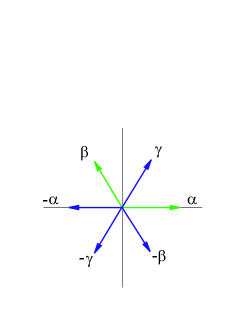
Figure 1: (Color online) The root diagram of $su(3)$.

Apart from the trivial one dimensional representation, where all the generators are assigned by the number $0$, there are a countably infinite number of unitary irreducible representations of $su(3)$. For any Lie algebra and any unitary representation of it say, $D$, there is a complex conjugate representation $\overline{D}$, where $\overline{D}(T)=[-D(T)]^{T}$. To see this one needs to invoke the fact that in a unitary representation of a group, the generators are represented by Hermitian matrices, so if $D(T_{a})$ satisfy the commutation relations of an algebra, so do $\overline{D}(T_{a}).$ As in the simpler case of $su(2)$, any representation of $su(3)$ is specified by its weights, that is the common eigenvalues of its vectors $|{\bf\mu}\rangle$ for the commuting operators $H_{1}$ and $H_{2}$;

$$H_{1}|{\bf\mu}\rangle=\mu_{1}|{\bf\mu}\rangle,\hskip 28.45274ptH_{2}|{\bf\mu}\rangle=\mu_{2}|{\bf\mu}\rangle.$$ (131)

There are two three dimensional representations which we denote simply by $3$ and $\overline{3}$. Their weight diagrams are shown in figure (2). Note that the weight diagram of $\overline{3}$ is obtained from that of $3$ by a reflection through the origin. The basis vectors of the $3$ representation are:

$$|\mu_{1}\rangle=|\frac{1}{2},\frac{1}{2\sqrt{3}}\rangle=\left(\begin{array}[]{c}1\\ 0\\ 0\end{array}\right),\ \ \ |\mu_{2}\rangle=|\frac{-1}{2},\frac{1}{2\sqrt{3}}\rangle=\left(\begin{array}[]{c}0\\ 1\\ 0\end{array}\right),\ \ \ |\mu_{3}\rangle=|0,\frac{-1}{\sqrt{3}}\rangle\left(\begin{array}[]{c}0\\ 0\\ 1\end{array}\right).$$ (132)

In such a representation the Cartan matrices are represented by

$$H_{1}=\frac{1}{2}\left(\begin{array}[]{ccc}1&&\\ &-1&\\ &&0\end{array}\right),\hskip 28.45274ptH_{2}=\frac{1}{2\sqrt{3}}\left(\begin{array}[]{ccc}1&&\\ &1&\\ &&-2\end{array}\right)$$ (133)

Similarly the basis vectors of the representation $\overline{3}$ are

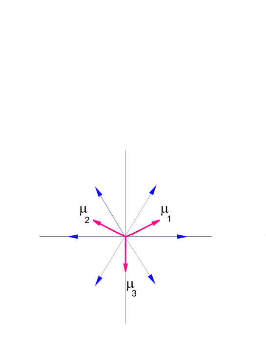
Figure 2: (Color online) The weight diagrams of the representations $3$ (left) and $\overline{3}$ (right).

$$|\overline{\mu}_{1}\rangle=|-\frac{1}{2},-\frac{1}{2\sqrt{3}}\rangle=\left(\begin{array}[]{c}1\\ 0\\ 0\end{array}\right),\ \ \ |\overline{\mu}_{2}\rangle=|\frac{1}{2},\frac{-1}{2\sqrt{3}}\rangle=\left(\begin{array}[]{c}0\\ 1\\ 0\end{array}\right),\ \ \ |\overline{\mu}_{3}\rangle=|0,\frac{1}{\sqrt{3}}\rangle\left(\begin{array}[]{c}0\\ 0\\ 1\end{array}\right).$$ (134)

In this representation, the Cartan matrices are represented by

$$H_{1}=\frac{1}{2}\left(\begin{array}[]{ccc}-1&&\\ &1&\\ &&0\end{array}\right),\hskip 28.45274ptH_{2}=\frac{1}{2\sqrt{3}}\left(\begin{array}[]{ccc}-1&&\\ &-1&\\ &&2\end{array}\right).$$ (135)

Other representations of small dimensions which we need for our discussions are $6$, $\overline{6}$, and $8$, where again the numbers denote dimensions of the representations. Note that a representation like $8$ is self-conjugate (real). The weight diagram of this representation is symmetric under reflection through the origin. Like $su(2)$, higher dimensional representations of $su(3)$ can be obtained simply by reducing the tensor product of the basic representations $3$ and $\overline{3}$. In particular it is well known that the tensor product of the basic representations decompose as follows [19]:

$$3\otimes 3 = 6\oplus\overline{3},$$ (136)

$$\overline{3}\otimes\overline{3} = \overline{6}\oplus 3,$$ (137)

$$3\otimes\overline{3} = 8\oplus 1,$$ (138)

$$\overline{3}\otimes 3 = 8\oplus 1.$$ (139)

There is a simple way for decomposing these representations based on symmetry under permutation. For example the basis states of $3\otimes 3$, are written as the sum of a symmetric and anti-symmetric combination, i.e.

$$|\mu_{i}\rangle|\mu_{j}\rangle=\frac{1}{2}(|\mu_{i}\rangle|\mu_{j}\rangle+|\mu_{j}\rangle|\mu_{i}\rangle)+\frac{1}{2}(|\mu_{i}\rangle|\mu_{j}\rangle-|\mu_{i}\rangle|\mu_{j}\rangle)$$ (140)

The symmetric multiplet forms the basis states of the representation $6$ and the antisymmetric multiplet that of $\overline{3}$. In a similar way, one can decompose $\overline{3}\otimes\overline{3}$ by writing $|\overline{\mu}_{i}\rangle|\overline{\mu}_{j}\rangle$ as a sum of a symmetric part ($\overline{6}$) and antisymmetric part ($3$). The decomposition of $3\otimes\overline{3}$ takes place by subtracting the trace part from the combination $|\mu_{i}\rangle|\overline{\mu}_{j}\rangle$ leaving us with an $8$ and a $1$, i.e.

$$|\mu_{i}\rangle|\overline{\mu}_{j}\rangle=(|\mu_{i}\rangle|\overline{\mu}_{j}\rangle-\frac{1}{3}\delta_{ij}\sum_{i}|\mu_{i}\rangle|\overline{\mu}_{i}\rangle)+\frac{1}{3}\delta_{ij}(\sum_{i}|\mu_{i}\rangle|\overline{\mu}_{i}\rangle).$$ (141)

References

• [1] E. C. G. Sudarshan, P. M. Mathews and J. Rau, Phys. Rev. 121, 920 (1961).
• [2] K. Kraus, States, Effects and Operations: Fundamental Notions of Quantum Theory, Springer, Berlin, 1983.
• [3] C. A. Rodr guez-Rosario, K. Modi, A. Kuah, A. Shaji, and E. C. G. Sudarshan, J. Phys. A: Math. Theor. 41 (2008) 205301.
• [4] M. A. Nielsen, and I. L. Chuang; Quantum computation and quantum information, Cambridge University Press, Cambridge, 2000.
• [5] M. B. Ruskai, S. Szarek, E. Werner, Lin. Alg. Appl. 347, 159 (2002)
• [6] A. Fujiwara, P. Algoet, Phys. Rev. A 59, 3290 (1999).
• [7] C. King, M. B. Ruskai, IEEE Trans. Info. Theory, 47 192 (2001).
• [8] G. Kimura, Phys. Lett. A 314, 339 (2003).
• [9] M. S. Byrd, N. Khanej, Phys. Rev. A 68, 062322 (2003).
• [10] I. P. Mendas, J. Math. Phys 49, 092102 (2008).
• [11] L. J. Boya, K. Dixit, Phys. Rev. A 78, 042108 (2008).
• [12] S. Kryszewski, M. Zachcia, J. Phys. A: Math. Gen. 39 5921 (2006).
• [13] A. Checinska, K. W odkiewicz, Phys. Rev. A 80, 032322 (2009).
• [14] M. S. Byrd, C. A. Bishop, Y. C. Ou, Phys. Rev. A 83, 012301 (2011).
• [15] A. S. Holevo, IEEE Trans. Info. Theory 44, 269-273 (1998).
• [16] A. S. Holevo, (2002), [ arxiv:0212025 [quant-ph]].
• [17] C. Macchiavello, G. M. Palma, and S. Virmani, Phys. Rev. A 69, 010303(R) (2004).
• [18] J. E. Humphreys, Introduction to Lie Algebras and representation theory, Springer (1973).
• [19] Georgi, Howard; Lie algebras in particle physics, Addison-Wesley publishing company, Canada, 1982.