Abstract

The famous equivalence theorem is reexamined in order to make it applicable to the case of effective theories. We slightly modify the formulation of this theorem and prove it basing on the notion of generating functional for Green functions. This allows one to trace (directly in terms of graphs) the mutual cancelation of different groups of contributions.

1 Introduction

The equivalence theorem (ET) is known since the early sixties [1] – [6]. Then, from time to time it was considered by different authors from various points of view (see, e.g., [7] – [13]). However, many practical aspects of this theorem remain unclear. In particular, the possibility to use it in the framework of effective theories still seems questionable. The point is that the very formulation of the equivalence theorem needs a refinement in order to adjust it to the case of effective theory.

Perhaps the most comprehensive consideration of this theorem along with the discussion of shortcomings in the previous proofs has been done in the papers [11], [13]. In those papers the ET is treated as the statement that $S$-matrix in quantum theory does not depend on the choice of variables in the corresponding classical Lagrangian. In other words, the canonical transformations in classical theory are considered as a kind of symmetry and the problem of the proof of ET thus reduces to that of conserving this symmetry in the process of quantization. Clearly, in this approach the form of classical Lagrangian cannot be arbitrary: the number of field derivatives must be at least finite. Moreover, the quantum theory under consideration must be renormalizable, otherwise the $S$-matrix would make no sense (both these points are specially stressed in [11]).

Meanwhile, the construction of effective theory is not based on any classical Lagrangian (or Hamiltonian), it is only restricted by the postulated structure of asymptotic states and the requirements of certain linear symmetry along with general principles like unitarity, causality (cluster decomposition) and Lorentz invariance of the $S$-matrix. As a consequence, the number (as well as the degree) of field derivatives appearing in the effective theory Hamiltonian is actually infinite. This makes the quantum theory renormalizable ab initio (see, e.g., [18]) but, at the same time, makes it impossible to point out the relevant classical Hamiltonian construction subjected to the quantization procedure. This means that the commonly accepted formulation (and, hence, proofs) of ET cannot be considered suitable in the case of effective theory. In this case one needs to prove a similar theorem (below we call it as modified equivalence theorem – MET) stating the perturbative equivalence of $S$-matrices in two inherently quantum theories with different Hamiltonians. Those Hamiltonians must be constructed from the same set of free field operators and connected with one another by certain transformation of the kind

$$\phi(x)\rightarrow\phi(x)+\alpha\sum_{k=2}^{\infty}\int\!\!\frac{1}{k!}\,F_{k}(x|y_{1},...,y_{k})\,\phi(y_{\scriptscriptstyle 1})\ldots\phi(y_{k})\,dy_{\scriptscriptstyle 1}\ldots dy_{k}\,.$$ (1)

Here $\alpha$ is just an auxiliary parameter and, by construction, $F_{n}(x|y_{\scriptscriptstyle 1},...,y_{k})$ is implied symmetric in arguments $y_{1},...,y_{k}$. There is no need in refereing to quantization of any particular classical theory. Note that usually the equivalence theorem is formulated for local transformations or, the same, for the case when

$$F_{k}(x|y_{\scriptscriptstyle 1},...,y_{k})\sim\prod_{i=1}^{k}\delta(x-y_{i})\,.$$

Here it is pertinent to note that the term “perturbative equivalence” makes no sense until the perturbation schemes for both theories are specified. Then, to compare the renormalized $S$-matrices in two theories one needs to perform the renormalization which, in turn, requires fixing the relevant renormalization prescriptions. At this point one meets a difficulty: the number of necessary prescriptions in two theories may prove to be different, at least, at first glance. Such a situation occurs, for example, when one performs the nonlinear change of field variables, say,

$$\phi\rightarrow F(\phi)=\phi+\alpha{\phi}^{2}$$

in the free field Lagrangian. The resulting Lagrangian contains the interaction term of the form ${\alpha}^{2}(\phi{\partial}_{\mu}\phi)^{2}$ and thus belongs to the class of non-renormalizable theories which require an infinite set of counterterms and the corresponding number of renormalization prescriptions. In fact, however, this is only true with respect to Green functions. It can be shown that the $S$-matrix in such a transformed theory remains trivial. Of course, the Green functions make no sense after removing the regularization.

The written above shows that, when formulating and proving the MET for the case of effective theory, one needs to trace the fine mutual cancellation of the contributions $\sim\alpha$ from all $S$-matrix graphs with a given number of external lines. There is no need in performing the complete renormalization – it is quite sufficient to prove this cancellation on the regularized $S$-matrix graphs (those with external lines on the mass shell). Surely, the proof must be based on the graph language. Attracting the functional integral technique is undesirable because in the case of effective theory the very definition of functional integral looks unconvincing: there is no classical action needed to construct it. Alternative definition – the formal sum of the loop perturbation series – also looks unacceptable because an infinite set of graphs with the same number of loops requires special ordering to avoid divergencies. Until this is done even the individual terms of loop series make no sense and, hence, their formal sum cannot be reasonably defined.

The paper is organized as follows. In Sec. 2 we explain our notations and give a list of formulae used throughout the paper. In Sec. 3 we give the precise formulation of MET statement. Sec. 4 is devoted to the proof of MET. It consists of 6 subsections. In Subsec. 4.1 we write down the generating functional $\widetilde{G}$ for Green functions of the transformed theory and show that it is connected with the functional $G$ of the initial one as follows: $\widetilde{G}=QG$. Here $Q$ is the variational operator functional fixed completely by the form of substitution law (1). Besides, it is shown that this operator takes the form of product of two series: determinant and exponential. In Subsec. 4.2 we consider the simplified example which helps one to understand the graphic technique needed to study the operator $Q$ structure. Then we list the set of graphic rules adjusted for the case of general transformation law (1). In Subsec. 4.3 we classify the types of graphs presenting the exponential series. Subsec. 4.4 is devoted to the analysis of graphic structure of determinant series. In Subsec. 4.5 it is shown that only one type (of three) of graphs survive in the series that presents the operator $Q$. Subsec. 4.6 completes the proof. Here we calculate the field strength renormalization constant $\widetilde{z}$ in transformed theory and show the absence of mass shift and tadpoles. Then we calculate renormalized $n$-point $S$-matrix element and demonstrate that it turns out the same as that in initial theory. Subsec. 5 contains the concluding remarks.

The variational functional formalism which we rely upon in this paper is not widely known. For this reason we find it pertinent to give a brief outlook of this formalism. This is done in Appendix A. Besides, when analyzing the structure of the operator $Q$ we make use of the first Mayer’s theorem [19]. The legality of this step is shown in Appendix B.

One note is in order. From the very beginning we work in the framework of renormalized perturbation scheme. Nevertheless, it is not difficult to check that the correctness of the result does not depend of this circumstance.

2 Preliminaries

In accordance with LSZ formula the renormalized $n$-particle $S$-matrix element can be obtained in four steps. First, one has to calculate the relevant Green function $G_{n}(x_{1},\ldots,x_{n})$. Second, every external line should be dotted by $D^{-1}$, where

$$D(x)=\frac{1}{(2{\pi})^{4}}\,\int\!\!dq\;{\rm exp}\{iqx\}\,D(q)\,,\ \ \ \ \ \ \ \ \ \ D(q)=\frac{i}{q^{2}-m^{2}+i0}\,,$$ (2)

and $D^{-1}$ – stands for the corresponding inverse operator. Third, every external line must be dotted by the factor $z^{\scriptscriptstyle-1/2}$ where $z$ is the field strength renormalization constant

$$z={\rm Res}\bigg{|}_{p^{2}=m^{2}}[-iG_{2}(p^{2})]=\left(1-\Sigma^{\prime}(p^{2})\bigg{|}_{p^{2}=m^{2}}\right)^{-1}$$ (3)

(here $G_{2}$ stands for the 2-point Green function while $\Sigma^{\prime}(p^{2})$ – for the self energy derivative with respect to $p^{2}$). At last, in the obtained expression one has to perform a transition to the mass shell.

So, only two last steps are connected with transition to the mass shell. For this reason on the first stage of our proof we concentrate solely on consideration of Green functions of transformed theory. The properties of renormalized $S$-matrix are studied on the second stage.

Before formulating and proving MET it is necessary to explain the notations used below. Throughout the paper we follow the monograph [20] and use shortened (matrix) notations omitting the integration symbols. For example, the expression $aDa$ should be understood as follows:

$$aDa\stackrel{{\scriptstyle\rm def}}{{=}}\int\!\!dxdy\,a(x)D(x-y)a(y).$$

Similarly, the operator expression $\delta_{a}D\delta_{a}$ means

$$\delta_{a}D\delta_{a}\stackrel{{\scriptstyle\rm def}}{{=}}\int\!\!dxdy\frac{\delta}{\delta a(x)}D(x-y)\frac{\delta}{\delta a(y)}\,.$$

Here the symbol

$$\delta_{a}\stackrel{{\scriptstyle\rm def}}{{=}}\frac{\delta}{\delta a}\stackrel{{\scriptstyle\rm def}}{{=}}\overrightarrow{\delta_{a}}$$ (4)

stands for the conventional left variational derivative acting to the right (‘L-derivative’). As usually,

$$Tr\,\,ln[1-{f^{\prime}}(a)]\stackrel{{\scriptstyle\rm def}}{{=}}-\int\!\!dx{f^{\prime}}(x;x|a)-\frac{1}{2}\int\!\!dxdy{f^{\prime}}(x;y|a){f^{\prime}}(y;x|a)-\ldots\,.$$ (5)

Hereafter the notation $f^{(n)}(x;y_{\scriptscriptstyle 1},\ldots,y_{n}|a)$ is used for the functional derivative of $f(x|a)$ with respect to $a(z)$:

$$f^{(n)}\equiv f^{(n)}(x;z_{\scriptscriptstyle 1},\ldots,z_{n}|a)\stackrel{{\scriptstyle\rm def}}{{=}}\frac{\delta^{n}f(x|a)}{\delta a(z_{\scriptscriptstyle 1})\ldots\delta a(z_{n})}\,,\ \ \ \ \ f^{\prime}\equiv f^{(1)}.$$ (6)

In what follows we call the first argument as the main index (or, the same, “main argument”) while ($z_{\scriptscriptstyle 1},\ldots,z_{n}$) placed between the semicolon and vertical line – as “induced”.

The generating functional of Green functions $G_{n}(x_{1},\ldots,x_{n})$ is defined as follows:

$$G(a)\stackrel{{\scriptstyle\rm def}}{{=}}\sum_{n=0}\frac{1}{n!}\int\!\!dx_{1}\ldots dx_{n}G_{n}(\ldots)a(x_{1})\ldots a(x_{n})\,.$$ (7)

Throughout the paper the notation $\phi(x)$ is used solely for free quantum field. The Latin letters are used for arbitrary classical fields.

We introduce two more variational differentiation operators in addition to the L-derivative defined by (4). The R-derivative $\overleftarrow{\delta_{a}}$ (acts from right to left) and LR-derivative $\overleftrightarrow{\delta_{a}}$ (the sum of L- and R- derivatives) are defined as follows:

$$f(a)\overleftarrow{\delta_{a}}g(a)\stackrel{{\scriptstyle\rm def}}{{=}}f^{\prime}(a)g(a)\,,$$ (8)

$$f(a)\overleftrightarrow{\delta_{a}}g(a)\stackrel{{\scriptstyle\rm def}}{{=}}f^{\prime}(a)g(a)+f(a)g^{\prime}(a).$$ (9)

It is easy to show that

$$\left[\overleftrightarrow{\delta_{a}},a\right]_{-}=0;\ \ \ \ \ \ \ \ \ \ \left[\overleftrightarrow{\delta_{a}},\overrightarrow{\delta_{a}}\right]_{-}=0\,.$$ (10)

So, to calculate the $S$-matrix elements one needs to calculate first the generating functional for Green functions (7) of the theory under consideration. This can be done with the help of relation (see [20]):

$$G(a)=\exp\left[V\!\left(\overrightarrow{\delta_{a}}\right)\right]\exp\left[\frac{1}{2}aDa\right]\cdot 1\,.$$ (11)

Here the symbol $\cdot 1$ is used to stress that the derivatives only operate on the second exponential: $\overrightarrow{\delta_{a}}\cdot 1=0.$ The variational functional

$$V(\overrightarrow{\delta_{a}})=V(b)\bigg{|}_{b=\overrightarrow{\delta_{a}}}\stackrel{{\scriptstyle\rm def}}{{=}}-i\int\!dx\,H_{int}^{\rm res}(b)\bigg{|}_{b=\overrightarrow{\delta_{a}}}$$ (12)

stands for the resultant functional image of symmetrized form (Sym-form) of quantum interaction Hamiltonian $H_{int}^{\rm res}(b)\,.$ The structure of this object is explained in [20] (brief explanations are also given in Appendix A below). In what follows there is no need to specify the construction of this functional.

3 Formulating the MET

In accordance with what is written in the previous Section (and in Appendix A) we work with the resultant image $V(a)$ that depends on arbitrary classical source field $a(x)$ (and with the corresponding variational functional $V(\delta_{a})$).

The MET statement is formulated as follows. Two quantum field theories with the resultant images $V(a)$ and $\widetilde{V}(a)$ lead to the same renormalized $S$-matrix under the condition that

$$\widetilde{V}(a)=V(a-f(a))+aD^{-1}f(a)-\frac{1}{2}\,f(a)D^{-1}f(a)+{\rm Tr}\,\,{\rm ln}[1-{f^{\prime}}_{\scriptscriptstyle a}(a)]\,.$$ (13)

Here $f(a)$ stands for the functional series (finite or formal infinite)

$$f(x|a)=\sum_{m=2}^{\infty}f_{m}(x|a)=\alpha\sum_{m=2}^{\infty}\frac{1}{m!}\int\!\!F_{m}(x|y_{\scriptscriptstyle 1},...,y_{m})\,a(y_{\scriptscriptstyle 1})\ldots a(y_{m})\,dy_{\scriptscriptstyle 1}\ldots dy_{m}\,,$$ (14)

where $\alpha$ is just a parameter. It is tacitly implied that the Fourier transform of $F_{m}(x|y_{1},...,y_{m})$ in $(y_{1},...,y_{m})$ does not contain negative powers of momenta.

Our proof of the above-formulated theorem is built upon the comparison of two functionals: $G(a)$ and $\widetilde{G}(a)$ constructed in accordance with (11) from $V$ and $\widetilde{V}$, respectively. This language allows us to trace in detail the effect of partial cancelation between groups of graphs that appear in the transformed theory and, at the same time, does not introduce any difficulties compared to the functional integral language used in [11]. We would like to stress that the problem of renormalizability has nothing to do with MET: the proof applies to regularized graphs irrelevantly to the possibility of removing regularization.

4 The proof

4.1 Step 1: the generating functional of transformed theory

According to the relation (11) the generating functional (7) for Green functions of transformed theory reads

$$\begin{split}\widetilde{G}(a)=\exp\left\{-\frac{1}{2}f\left(\overrightarrow{\delta_{a}}\right)D^{-1}f\left(\overrightarrow{\delta_{a}}\right)+V\left[\overrightarrow{\delta_{a}}-f\left(\overrightarrow{\delta_{a}}\right)\right]+f\left(\overrightarrow{\delta_{a}}\right)D^{-1}\overrightarrow{\delta_{a}}\right\}\\ \times\exp\left\{{\rm Tr}\,{\rm ln}\left(1-f_{a}^{\prime}\left(\overrightarrow{\delta_{a}}\right)\right)\right\}\exp\left[\frac{1}{2}aDa\right]\cdot 1\,.\end{split}$$ (15)

In this Section we will show that this expression can be rewritten as follows

$$\widetilde{G}(a)=\exp\left\{{\rm Tr}\,{\rm ln}\left(1-f_{a}^{\prime}\left(\overrightarrow{\delta_{a}}\right)\right)\right\}:\exp\left[af(\overrightarrow{\delta_{a}})\right]:G(a)\stackrel{{\scriptstyle\rm def}}{{=}}Q\left(a,\overrightarrow{\delta_{a}}\right)\,G(a).$$ (16)

The notation $:\ldots:$ (“anti-normal form”) should be read as follows

$$:\exp\left[f\left(\overrightarrow{\delta_{a}}\right)a\right]\!:\stackrel{{\scriptstyle\rm def}}{{=}}\sum_{n=0}^{\infty}\frac{1}{n!}f^{n}\left(\overrightarrow{\delta_{a}}\right)a^{n}.$$ (17)

The relations (8), (9) and (10) allow one to change the direction of arrows above certain operators $\overrightarrow{\delta_{a}}$ in (15) and rearrange them as follows (recall that $1\cdot\overleftarrow{\delta_{a}}=\overrightarrow{\delta_{a}}\cdot 1=0$):

$$\begin{split}\widetilde{G}(a)=1\cdot{\cal D}\cdot{\cal F}\cdot\exp{V\left[\overrightarrow{\delta_{a}}-f\left(\overleftrightarrow{\delta_{a}}\right)\right]}\exp{\left[f\left(\overleftrightarrow{\delta_{a}}\right)D^{-1}\overrightarrow{\delta_{a}}\right]}\exp\left[\frac{1}{2}aDa\right]\cdot 1{}\,.\end{split}$$ (18)

Here

$${\cal D}\stackrel{{\scriptstyle\rm def}}{{=}}\exp\left\{{\rm Tr}\,\,{\rm ln}\left[1-f_{a}^{\prime}\left(\overleftrightarrow{\delta_{a}}\right)\right]\right\}={\rm det}\left[1-f_{a}^{\prime}\left(\overleftrightarrow{\delta_{a}}\right)\right]$$ (19)

and

$${\cal F}\stackrel{{\scriptstyle\rm def}}{{=}}\exp\left\{-\,\frac{1}{2}f\left(\overleftrightarrow{\delta_{a}}\right)D^{-1}f\left(\overleftrightarrow{\delta_{a}}\right)\right\}.$$ (20)

Because $f(\overleftrightarrow{\delta_{a}})$ commutes with $a$ one can make use of the identity

$$\exp\left[h\overrightarrow{\delta_{a}}\right]F(a)\cdot 1=F(a+h)\,,$$ (21)

and rewrite two last exponentials in (18) as follows:

$$\begin{split}\exp&\left[f\left(\overleftrightarrow{\delta_{a}}\right)D^{-1}\overrightarrow{\delta_{a}}\right]\exp\left[\frac{1}{2}aDa\right]\cdot 1=\\ =&\exp\left\{\frac{1}{2}\left[a+f\left(\overleftrightarrow{\delta_{a}}\right)D^{-1}\right]D\left[a+f\left(\overleftrightarrow{\delta_{a}}\right)D^{-1}\right]\right\}\cdot 1=\\ =&\exp\left[\frac{1}{2}f\left(\overleftrightarrow{\delta_{a}}\right)D^{-1}f\left(\overleftrightarrow{\delta_{a}}\right)\right]\exp\left[af\left(\overleftrightarrow{\delta_{a}}\right)\right]\exp\left(\frac{1}{2}aDa\right)\cdot 1=\\ =&\,{\cal F}^{-1}\exp\left[af\left(\overleftrightarrow{\delta_{a}}\right)\right]\exp\left(\frac{1}{2}aDa\right)\cdot 1\,.\end{split}$$ (22)

The last equality follows from the definition (20). Substituting (22) in (18) we obtain

$$\widetilde{G}(a)=1\cdot{\cal D}\cdot\exp{V\left[\overrightarrow{\delta_{a}}-f\left(\overleftrightarrow{\delta_{a}}\right)\right]}\exp\left[af\left(\overleftrightarrow{\delta_{a}}\right)\right]\exp\left(\frac{1}{2}aDa\right)\cdot 1\,.$$ (23)

Let us now make use of another identity, namely,

$$F\left(\overrightarrow{\delta_{a}}\right)\exp[ha]\cdot\Phi(a)=\exp[ha]F\left(\overrightarrow{\delta_{a}}+h\right)\cdot\Phi(a)\,.$$ (24)

It allows one to rewrite (23) as follows

$$\begin{split}\widetilde{G}(a)=&1\cdot{\rm det}\left[1-f_{a}^{\prime}\left(\overleftrightarrow{\delta_{a}}\right)\right]\exp\left[af\left(\overleftrightarrow{\delta_{a}}\right)\right]\exp\left[V\left(\overrightarrow{\delta_{a}}\right)\right]\exp\left(\frac{1}{2}aDa\right)\cdot 1\,\,.\end{split}$$ (25)

The relations (10) allow one to change the direction of arrows in (25). Indeed,

$$\begin{split}\widetilde{G}(a)=\,\,&1\cdot{\rm det}\left[1-f_{a}^{\prime}\left(\overleftrightarrow{\delta_{a}}\right)\right]\sum_{k=1}^{\infty}\frac{1}{k!}\left[af\left(\overleftrightarrow{\delta_{a}}\right)\right]^{k}G(a)\equiv\\ \equiv\,\,&1\cdot{\rm det}\left[1-f_{a}^{\prime}\left(\overleftrightarrow{\delta_{a}}\right)\right]\sum_{k=1}^{\infty}\frac{1}{k!}\left[f\left(\overleftrightarrow{\delta_{a}}\right)\right]^{k}a^{k}\,\,G(a)\stackrel{{\scriptstyle\rm def}}{{=}}\\ \stackrel{{\scriptstyle\rm def}}{{=}}\,\,&1\cdot{\rm det}\left[1-f_{a}^{\prime}\left(\overrightarrow{\delta_{a}}\right)\right]:\exp\left[f\left(\overrightarrow{\delta_{a}}\right)a\right]\!:G(a)\,.\end{split}$$ (26)

Here the account was taken of the relation (11). So, we obtain finally

$$\widetilde{G}(a)=1\cdot{\rm det}\left[1-f_{a}^{\prime}\left(\overrightarrow{\delta_{a}}\right)\right]:\exp\left[f\left(\overrightarrow{\delta_{a}}\right)a\right]\!:G(a)\equiv Q\left(a,\overrightarrow{\delta_{a}}\right)\,G(a)\,.$$ (27)

Now the relation (16) is obtained and the first step is done. Recall that both the determinant and exponential are just shortened notations for corresponding operator series.

Our next goal is to bring the operator $Q\left(a,\overrightarrow{\delta_{a}}\right)$ to the “normal” form where all source fields $a(x)$ are placed in front of all variational operators $\delta_{a}$.

4.2 Step 2: the operator graphic technique

Let us now turn to a consideration of the structure of operator

$$Q\left(a,\overrightarrow{\delta_{a}}\right)\stackrel{{\scriptstyle\rm def}}{{=}}1\cdot{\rm det}\left[1-f_{a}^{\prime}\left(\overrightarrow{\delta_{a}}\right)\right]:\exp\left[f\left(\overrightarrow{\delta_{a}}\right)a\right]:\,.$$ (28)

This will require developing the special graphic technique which, however, has nothing to do with conventional Feynman graphs of the quantum theory in question.

To do this step by step we first consider the exponential series (17). The simple example discussed below allows one to better understand the graphical structure of this series.

Suppose that the sum in (14) contains only one term

$$f_{m}(x|a)=0,\ \ \ \ (m\neq k).$$ (29)

For simplicity we took $\alpha=1$. In this case the exponential under consideration takes the form (here $\vec{y}_{i}\stackrel{{\scriptstyle\rm def}}{{=}}(y_{i\!{\scriptscriptstyle 1}},\ldots,y_{ik}).$)

$$:\exp\left[f\left(\overrightarrow{\delta_{a}}\right)a\right]:\,\,=\sum_{n=0}^{\infty}e_{n}=\sum_{n=0}^{\infty}\frac{1}{n!}\int\!\!dx_{\!\scriptscriptstyle 1}\ldots dx_{n}d\vec{y}_{\scriptscriptstyle 1}\ldots d\vec{y}_{n}\left(\frac{1}{k!}\right)^{n}\,\times\\ F_{k}(x_{\!\scriptscriptstyle 1}|\vec{y}_{\scriptscriptstyle 1})\ldots F_{k}(x_{n}|\vec{y}_{n})\frac{\overrightarrow{\delta}}{\delta a(y_{\!\scriptscriptstyle 1\!1})}\ldots\frac{\overrightarrow{\delta}}{\delta a(y_{{\!\scriptscriptstyle 1}k)}}\ldots\frac{\overrightarrow{\delta}}{\delta a(y_{n{\!\scriptscriptstyle 1}})}\ldots\frac{\overrightarrow{\delta}}{\delta a(y_{nk})}a(x_{\!\scriptscriptstyle 1})\ldots a(x_{n})\,.$$ (30)

This expression should be brought into the normal form which can be easily interpreted graphically. First of all let us reduce the first nontrivial term to the form where the source field $a$ stands before all differentiation operators. This gives

$$e_{1}=:\left[f\left(\overrightarrow{\delta_{a}}\right)a\right]:\,\,\equiv\,\,\int\!dx_{\!\scriptscriptstyle 1}\frac{1}{k!}\int\!d\vec{y}_{\scriptscriptstyle 1}\,F_{k}(x_{\!\scriptscriptstyle 1}|\vec{y}_{\!\scriptscriptstyle 1})\frac{\overrightarrow{\delta}}{\delta a(y_{\!\scriptscriptstyle 11})}\ldots\frac{\overrightarrow{\delta}}{\delta a(y_{\!{\scriptscriptstyle 1}k})}a(x_{1})\,=\\ \int\!dx_{\!\scriptscriptstyle 1}\left\{\frac{1}{k!}\,\int\!d\vec{y}_{\scriptscriptstyle 1}F_{k}(x_{\!\scriptscriptstyle 1}|\vec{y}_{\!\scriptscriptstyle 1})\left[\sum_{i=1}^{k}\delta(x_{\!\scriptscriptstyle 1}-y_{{\!\scriptscriptstyle 1}i})\prod_{r=1\atop r\neq i}^{k}\frac{\overrightarrow{\delta}}{\delta a(y_{{\!\scriptscriptstyle 1}r})}\right]\,+\,\right.\\ \left.a(x_{\!\scriptscriptstyle 1})\frac{1}{k!}\int\!d\vec{y}_{\!\scriptscriptstyle 1}\,F_{k}(x_{\!\scriptscriptstyle 1}|\vec{y}_{\!\scriptscriptstyle 1})\frac{\overrightarrow{\delta}}{\delta a(y_{\!\scriptscriptstyle 11})}\ldots\frac{\overrightarrow{\delta}}{\delta a(y_{{\!\scriptscriptstyle 1}k})}\right\}\,\equiv\,\\ \int\!dx_{\!\scriptscriptstyle 1}\left[f^{\prime}(x_{\!\scriptscriptstyle 1};x_{\!\scriptscriptstyle 1}|\overrightarrow{\delta_{a}})\,+\,a(x_{\!\scriptscriptstyle 1})f(x_{\!\scriptscriptstyle 1}|\overrightarrow{\delta_{a}})\right]\,.$$ (31)

Note that the first term in the last line of (31) results from the integrating with relevant $\delta$-functions and accounting for the symmetry of $F_{k}(x|y_{\scriptscriptstyle 1},\ldots,y_{k})$ in arguments $(y_{\scriptscriptstyle 1},\ldots,y_{k})$. Note, also, that in this term the induced argument coincides with the main one.

To better understand the structure of higher terms of the series (17) let us calculate the third term

$$e_{2}=\frac{1}{2!}\int\!\!dx_{\scriptscriptstyle 1}dx_{\scriptscriptstyle 2}d\vec{y_{\scriptscriptstyle 1}}d\vec{y_{\scriptscriptstyle 2}}F_{2}(x_{\scriptscriptstyle 1}|\vec{y_{\scriptscriptstyle 1}})F_{2}(x_{\scriptscriptstyle 2}|\vec{y_{\scriptscriptstyle 2}})\frac{\overrightarrow{\delta}}{\delta a(y_{\scriptscriptstyle 11})}\frac{\overrightarrow{\delta}}{\delta a(y_{\scriptscriptstyle 12})}\frac{\overrightarrow{\delta}}{\delta a(y_{\scriptscriptstyle 21})}\frac{\overrightarrow{\delta}}{\delta a(y_{\scriptscriptstyle 22})}a(x_{\scriptscriptstyle 1})a(x_{\scriptscriptstyle 2})$$

of the expansion (30) using the compact notations (6) (for brevity we consider the case $k=2$).

This gives (the integrating over repeating arguments $x_{1},x_{2}$ is implied; the operator arguments $\overrightarrow{\delta_{a}}$ are not shown):

$$e_{2}=\frac{1}{2!}f_{2}(x_{1}|)f_{2}(x_{2}|)a(x_{1})a(x_{2})=\frac{1}{2!}f_{\scriptscriptstyle 2}(x_{1}|)\left[a(x_{1})f_{2}(x_{2}|)+f_{2}^{(1)}(x_{2};x_{1}|)\right]a(x_{2})=\ldots=\\ \frac{1}{2!}\left\{a(x_{1})a(x_{2})f_{2}(x_{1}|)f_{2}(x_{2}|)+a(x_{2})f_{2}^{(1)}(x_{1};x_{1}|)f_{2}(x_{2}|)+a(x_{1})f_{2}^{(1)}(x_{2};x_{2}|)f_{2}(x_{1}|)+\right.\\ \left.f_{2}^{(1)}(x_{1};x_{1}|)f_{2}^{(1)}(x_{2};x_{2}|)+a(x_{1})f_{2}^{(1)}(x_{1};x_{2}|)f_{2}(x_{2}|)+a(x_{2})f_{2}^{(1)}(x_{2};x_{1}|)f_{2}(x_{1}|)+\right.\\ \left.f_{2}^{(1)}(x_{1};x_{2}|)f_{2}^{(1)}(x_{2};x_{1}|)+f_{2}(x_{2}|)f_{2}^{(2)}(x_{1};x_{1},x_{2}|)+f_{2}(x_{1}|)f_{2}^{(2)}(x_{2};x_{1},x_{2}|)\right\}.\qquad$$ (32)

Here the relation

$$f^{(p)}_{k}(x_{i};z_{i{\scriptscriptstyle 1}},\ldots,z_{ip}|)a(x_{r})=a(x_{r})f^{(p)}_{k}(x_{i};z_{i{\scriptscriptstyle 1}},\ldots,z_{ip}|)+f^{(p+1)}_{k}(x_{i}\,;x_{r},z_{i{\scriptscriptstyle 1}},\ldots,z_{ip}|)$$ (33)

has been multiply used.

The above considered examples allow one to formulate simple rules needed to present the exponential series in graphic form. Indeed, calculating higher terms of the expansion (30) ($e_{\scriptscriptstyle 3}$, $e_{\scriptscriptstyle 4}\ldots$) we see that the result always takes a form of sum of products of independent (“disconnected”) integrals over repeating arguments of relevant factors (in operator graphic language – vertices, or, more precisely, vertex variational functionals). Let us consider the graphic structure of individual independent integrals (“connected graphs”). For this it is necessary to formulate the set of rules needed to present the terms of the expansion (17) (under the condition (29)) in graphical form. This set reads:

1. The $n$th order term is presented by the sum of oriented graphs (both connected and disconnected). Every individual item (graph) of this sum has $n$ vertices marked by the main arguments of relevant vertex factors.

2. Every connected graph consists of vertices, oriented propagator lines (propagators) connecting the vertices with one another or a given vertex with itself, and free lines of two kinds: outgoing and incoming. The analytical form corresponding to a given connected graph should be constructed in accordance with the rules listed below.

3. Every vertex has one incoming line and $k$ outgoing ones.

4. The vertex marked by its main index $x_{\scriptscriptstyle 1}$ with $p$ outgoing propagator lines (which connect it with vertices marked by $z_{\scriptscriptstyle 1},\ldots,z_{p}$), $(k-p)$ outgoing free lines and one incoming line (the type of which is immaterial) corresponds to the non-local variational operator expression

   $$f_{k}^{(p)}(x_{\scriptscriptstyle 1};z_{\scriptscriptstyle 1},\ldots,z_{p}|).$$

5. The incoming free line (of the vertex marked by $x_{r}$) corresponds to $a(x_{r})$.

6. The propagator line is oriented: it starts at the vertex with index $x_{k}$ and ends at that with index $x_{l}$. This means that one of induced arguments of the vertex marked by $x_{k}$ coincides with $x_{l}$. The corresponding factor is just a unity.

7. The integration over the main indices of all vertices is implied.

8. Every graph of $n$th order should be dotted by the factor $1/n!$ appearing in the exponential series.

9. To avoid confusion one should arrange the product of factors associated with elements of a given graph such that the source field $a(x_{i})$ is placed first.

The graphical representations of the expressions (31) and (32) are shown on Figs. 1 and 2, respectively.

Clearly, if the function $f(x|a)$ is defined by the general relation (14), the corresponding complex vertex are constructed as direct sum of elementary ones described above. Such a composite vertex can be drawn as a bullet (see Fig. 3).

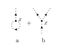
Figure 1: The graphical representation of the terms in the fourth line of (31).

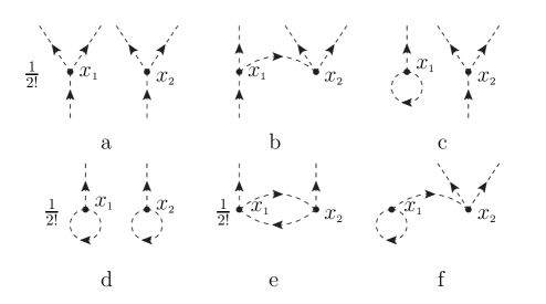
Figure 2: The third term of the series (30). The integral over $x_{\scriptscriptstyle 1}$ and $x_{\scriptscriptstyle 2}$ is implied.

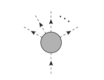
Figure 3: Non-local composite vertex.

From the above-listed rules it follows that: 1) Connected graph can have at most one incoming line; 2) The connected graph cannot have more than one loop; 3) The one-loop graphs have no incoming line or, the same, such graphs do not contain the source field $a(x)$.

The given above set of compact graphic rules is convenient just because every connected graph presents nothing but a product of relevant vertex factors (integrated over their main indices), the factor that contains the source field $a(x_{i})$ being placed in front of all others.

It seems us pertinent to note that in often discussed case when the function $F_{n}$ is taken singular

$$F_{n}(x|y_{\!\scriptscriptstyle 1}\ldots y_{n})\sim\prod_{i=1}^{n}\delta(x-y_{i})$$

the loop graphs become singular and one needs to introduce regularization. This fact is usually neglected. Nevertheless, this is not a mistake. Below we will prove that the loop graphs stemming from the determinant series cancel those stemming from exponential. This means that the result does not depend on the type of regularization chosen. In our approach the regularization appears in natural way: it is provided by non-local character of the transformation law (1).

4.3 The exponential series: general structure

The discussion in previous Subsection allows one to conclude that the exponential series (17) results in three different types of connected operator graphs:

• Trees. They have one incoming line, the others are outgoing (like the graph b in Fig. 2). This means that each of these graphs contains the field $a$ surviving after all variational derivatives inside the exponential are done.

• One particle irreducible (1PI) one loop graphs (“garlands”). These graphs have no incoming lines coordinated with the source field (see, e.g., the graph e and every one of two subgraphs d on Fig. 2).

• 1PI one loop graphs connected to some number of tree graphs (e.g., the graph f of the sum presented on Fig. 2). This kind graphs also have only outgoing lines.

Recall that the exponential does not produce connected graphs with the number of loops $l>1$.

4.4 The determinant series

Let us now turn to a consideration of the determinant series

$${\cal D}=\exp\left\{{\rm Tr}\,\,{\rm ln}\left[1-f_{a}^{\prime}\left(\overrightarrow{\delta_{a}}\right)\right]\right\}.$$ (34)

As it follows from (5) and the listed above set of compact graphic rules, the expression (34) can be graphically presented in the form of an infinite series of disconnected garlands. Every garland has the same vertices and is constructed precisely in the same way as the above-described graph of the type B. The first nontrivial term in the series (34) reads

$$-\sum_{k=1}^{\infty}\frac{1}{k}\,\,L_{k}\,,$$ (35)

where $L_{k}$ stands for the garland with $k$ vertices.

4.5 The operator Q series

From the written above it follows that the operator $Q$, which is the product of two series – determinant and exponential, results precisely in the same graphs as those stemming from the exponential; the only difference is connected with the values of combinatorial factors. Indeed, the garlands from the determinant series only may act on trees produced by exponential – they commute with exponential loop graphs just because the latter ones have no incoming arrows.

Let us show now that, in fact, only the graphs of the type A survive in this product: the loop graphs cancel each other. For this it is sufficient to show that the sum of connected graphs $W(\overrightarrow{\delta_{a}},a)$ does not contain loop contributions.

First of all, it is clear that the $k$-vertex graphs of the type B (garlands) stemming from the determinant completely cancel those from the exponential. This follows from the comparison of relevant symmetry factors: as pointed above (see (35)) the symmetry factor of the determinant garland equals $-1/k$ while that of the exponential one is $1/k$. The latter value results from the product of two factors: the numerical coefficient $1/k!$ that appears in the exponential series and $(k-1)!$ provided by the garland-type contribution from the operator term $:\!\prod_{i=1}^{k}f(x_{i}|\overrightarrow{\delta_{a}})a(x_{i})\!:.$ Recall that we only consider the connected graphs.

Next, let us consider the type C graphs with only one $l$-vertex tree (“tail”) connected to the $k$-vertex garland. There are two different sources of such kind graphs. First, as explained above, they appear in the exponential series. The corresponding combinatorial factor we denote as $S_{exp}^{C}(k,l)$. Second, they appear as the result of acting the $k$-vertex garland from determinant on the relevant $l$-vertex tree from exponential (graph f on Fig. 2). The symmetry factor for the graph stemming from this latter source we denote as $S_{d-e}^{C}(k,l)$. We need to show that

$$S_{exp}^{C}(k,l)=-S_{d-e}^{C}(k,l).$$ (36)

It is not difficult to show that the symmetry coefficient for $k$-vertex garland equals $1/k$. The detailed structure of the $l$-vertex tree graph (the number of its branches) is not essential for the further analysis. Suppose its combinatorial factor is $S^{A}(l)$. Then the factor $S_{exp}^{C}(k,l)$ reads:

$$S_{exp}^{C}(k,l)=\frac{1}{(l+k)!}\,C^{k}_{l+k}\,(k-1)!\,k\,S^{A}(l)=S^{A}(l).$$ (37)

Here the multiplier $C^{k}_{l+k}$ accounts for the possibility to choose $k$ vertices needed to construct the garland from $(k+l)$ ones, $1/(k+l)!$ stems from the exponential series, while the meaning of $(k-1)!$ is explained above. At last, the factor $k$ accounts for the possibility to choose one of $k$ vertices of the garland which the tree is connected to.

Let us now compute the factor $S_{d-e}^{C}(k,l)$. Taking account of (35) we obtain

$$S_{d-e}^{C}(k,l)=-\,S^{A}(l)\,k\frac{1}{k}=-\,S_{exp}^{C}(k,l).$$ (38)

Here the factor $k$ appears due to the same reason as in (37) while $1/k$ is the symmetry coefficient of a garland. This shows that the relation (36) is true in the case of one-tail garlands. The generalization to the case of garlands with many tails is straightforward.

4.6 Step 3: mass shift, tadpoles and the field renormalization constant

In this Subsection we closely follow the reasoning of [11]. As shown above, the graphs for $\widetilde{G}(a)$ result from the action of the series of operator trees stemming from the exponential on the graphs of generating functional $G(a)$ of the initial theory. Therefore the typical graph of the $n$-point Green function $\widetilde{G}_{n}(x_{1},\ldots,x_{n})$ of transformed theory appears as that presented on Fig. 4.

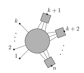
Figure 4: The typical connected Green function graph of transformed theory. It is implied that the circle corresponds to the full (containing both strongly and weakly connected parts) connected Green function of the initial theory..

On that Figure the circle corresponds to the connected (amputated) Green function of the initial theory while squares present the full sum of operator trees (the type A graphs described in Sec. 4). It is implied summation over the number of operator subgraph legs.

It is clear that the only type of Green function graphs providing nontrivial contribution to $n$-particle $S$-matrix elements of transformed theory is that presented on Fig. 5

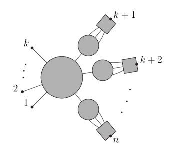
Figure 5: Green function graph with $\sigma$-legs.

with $k=0,1,\ldots,n$. These graphs have two kinds of legs:

• ‘Conventional’ legs each of which corresponds to the full propagator of initial theory (on Fig. 4 they are marked by numbers $1,2,\ldots,k$).

• The so-called $\sigma$-legs (marked by numbers $k+1,k+2,\ldots,n$ on Fig. 4). Every one of such legs presents the 2-point $\sigma$-graph (shown on Fig. 6) weakly connected to the rest part of the whole graph in question. We would like to stress that, by construction, $\sigma$-graphs have no poles in $p^{2}$.

  

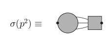
  Figure 6: The structure of $\sigma$-graph. By construction, it has no pole in $p^{2}$.

To calculate the renormalized $S$-matrix in transformed theory we need first to consider two point Green function $\widetilde{G}_{2}$ in order to find its pole position and the corresponding residue. The relevant sum of graphs is shown on the Fig. 7. Recall that every solid line corresponds to the full propagator of the initial theory and all vertices are implied full. In other words, every graph depicted in Fig. 7 presents an infinite series. Note that the last graph in this sum is one particle irreducible.

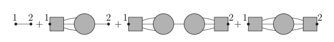
Figure 7: Full 2-point Green function $\widetilde{G_{2}}(p^{2})$.

Let us now suppose that the pole of full two point Green function of the initial theory is located at $p^{2}=m^{2}$. From Fig. 7 it follows immediately that the pole position of two point function $\widetilde{G}_{2}(p^{2})$ of transformed theory remains unchanged – the mass shift is absent.

Similar analysis shows that the tadpole graphs do not appear in the transformed theory if – as we tacitly imply – they were absent (due to relevant renormalization condition) in the initial one.

Further, denoting the $\sigma$-graph (Fig. 6) at $p^{2}=m^{2}$ as $\sigma$ one can present the expression for the residue of the full propagator of transformed theory (see Fig. 7; note that only the first three graphs contribute, the second one having the symmetry factor 2) as follows:

$${\rm Res}\,\widetilde{G}_{2}\bigg{|}_{p^{2}=m^{2}}=i\left[1+2\sigma+{\sigma}^{2}\right]\cdot{\rm Res}\,G_{2}\bigg{|}_{p^{2}=m^{2}}\,.$$ (39)

Therefore the field strength renormalization constant in the transformed theory differs from that in the initial one; it reads:

$$\widetilde{z}=-i\,{\rm Res}\,\widetilde{G}_{2}\bigg{|}_{p^{2}=m^{2}}=z\,[1+\sigma]^{2}\,.$$ (40)

Let us now consider the new renormalized $S$-matrix. The connected $n$-leg $S$-matrix graph in the transformed theory can be obtained from the $n$-point Green function graph $\widetilde{G}_{n}$ with the help of substitution

$$a_{i}\longrightarrow\widetilde{z}^{-1/2}D^{-1}(p_{i})$$ (41)

and subsequent taking the limit $p_{i}^{2}\rightarrow m^{2}.$ This results in disappearance of factors $D$ from external lines and from $\sigma$-legs. Besides, this introduces the common factor $\widetilde{z}^{-n/2}.$ As is seen from Fig. 5, the resulting factor that appears after summing graphs with different number of $\sigma$-legs reads:

$$\widetilde{N}=\widetilde{z}^{-n/2}\sum_{k=0}^{n}C_{n}^{k}\sigma^{k}=[1+\sigma]^{n}z^{-n/2}[1+\sigma]^{-n}=z^{-n/2}\,.$$ (42)

Here the multiplier $C_{n}^{k}$ accounts for various possibilities to choose the $(n-k)$ $\sigma$-legs from the total number $n$ of legs of the graph in question.

Thus it is shown that (the symbol $\widetilde{G}_{n}(k)$ stands for $n$-point Green function with $k$ $\sigma$-legs)

$$\widetilde{z}^{-n/2}\sum_{k=0}^{n}\widetilde{G}_{n}(k)=z^{-n/2}G_{n}.$$ (43)

From this it follows immediately that the renormalized $n$-leg $S$-matrix graphs in two theories (initial and transformed) coincide identically. In other words, these two theories result in the same renormalized $S$-matrix:

$$\widetilde{S}^{\rm ren}=S^{\rm ren}$$

This proves the theorem under consideration.

5 Concluding remarks

As we have already mentioned in Sec 1, the very formulation of the proved above theorem differs from that considered previously in the literature (see, e.g., [11], [13]). For this reason it makes sense to discuss the consequences in more detail.

1. Our proof is not connected with any quantization scheme. It is not connected with the structure of classical field theory at all. We work directly with the quantum interaction Hamiltonian in the interaction picture and rely upon the conventional perturbation scheme (Dyson’s $T$-exponential presented in the form of generating functional for Green functions). This makes the MET applicable for the case of effective theory.

2. Our treatment – in contrast to the conventional one – is well suited for a consideration of “good enough” non-local field transformations. This is especially important in effective theories which are non-local by their very construction.

3. The above-given proof does not require using the functional integral technique which looks unconvincing in the case of effective theory. For this reason our result may be considered as independent proof of the admissibility of changing variables in the formally written functional integral that depends on the special kind of source function.

4. It is pertinent to note that the substitution of the form (14) adds an additional set of parameters to that presented in the initial theory. For this reason when comparing two $S$-matrices one needs to work within the perturbation scheme defined by the initial theory. In this case, as it follows from our proof, all the terms depending on new parameters, will disappear at every order of the initial perturbation expansion.

5. Clearly, our proof can be easily generalized for the case of infinite number of scalar (and spinor) fields.

At last we would like to mention the idea first suggested by Veltman [22]. In that paper it was shown that the local (very simple) theory of one stable and one unstable particle with masses $m$ and $M>2m$, respectively, can be reformulated solely in terms of the stable particle field with non-local Lagrangian. The resulting $S$-matrix, defined on the space of asymptotic states of stable particles, turns out to be unitary and causal; its elements are the same as the corresponding $S$-matrix elements in initial (simple and local) theory. Does it mean that one can find, at least in principle, the equivalent transformation of a local theory with stable particle $\phi$ and resonance $\kappa$ to the non-local one only containing the $\phi$ field? It seems us interesting to explore such a possibility. The MET may turn out to be a useful tool for this purpose.

Appendix A

Since the variational functional technique described in the monograph [20] is not as widely known as, say, the functional integral, it seems pertinent to devote this Appendix to brief outline of certain aspects which we rely upon in the main text.

First we have to remind what is Sym-form. The precise definition of Sym-form of operator product looks as follows:

$${\rm Sym}\left[Q_{1}Q_{2}\ldots Q_{n}\right]\stackrel{{\scriptstyle\rm def}}{{=}}\frac{1}{n!}\sum_{P}\varepsilon_{\scriptscriptstyle P}P\left[Q_{1}Q_{2}\ldots Q_{n}\right].$$

Here summation runs over all $n!$ permutations $P$ of the operators $Q_{i}$ while $\varepsilon_{\scriptscriptstyle P}$ is nothing but conventional statistical factor (-1 for permutation of two fermionic operators and +1 for bosonic ones). The above definition along with many useful relations connecting Sym-product with T- (time-ordered) and N- (normal-ordered) products can be found in [20]. The usefulness of using the Sym-form of quantum Hamiltonian follows from the possibility to exploit the variational form of Wick theorems first suggested in [21].

Let us now outline the relation between two methods – quantum and variational classical – of calculating Green functions. Let $H(\phi)$ be the quantum interaction Hamiltonian (depending on free quantum field $\phi$ and its derivatives and containing all necessary counterterms). The well known Dyson T-exponential together with Wick theorems allow one to establish Feynman rules and to calculate Green functions. This can be done in two ways. The first way is to rely upon quantum commutation relations and use Wick theorems in their original form. The second one consists of rewriting those theorems in terms of classical (commuting or, in case of fermions, anticommuting) objects (Hori’s theorems [21]) and subsequent reformulating the formalism of Green function calculations. It is this latter way which we briefly describe below.

The variational language allows one to perform the calculation of Green functions operating with classical objects. For this it is necessary to present $H(\phi)$ in Sym-form. Suppose this is already done:

$$H(\phi)\stackrel{{\scriptstyle\rm def}}{{=}}H^{\rm Sym}_{int}(\phi)={\rm Sym}H(\phi).$$ (44)

To make use of the relations (11) and (12) one needs to construct the resultant image $H_{int}^{\rm res}(b)$ of $H^{\rm Sym}_{int}(\phi).$ This can be done as follows. First, define the time derivatives of free quantum field $\phi$ as new independent quantum fields

$$\frac{{\partial}^{k}\phi}{{\partial t}^{k}}\stackrel{{\scriptstyle\rm def}}{{=}}{\phi}_{k}\,.$$ (45)

Second, calculate the relevant Dyson and Wick contractions $D_{mn}^{\scriptscriptstyle D}$ and $D_{mn}^{\scriptscriptstyle W}$ and corresponding differences

$$\alpha_{mn}\equiv D_{mn}^{\rm{\scriptscriptstyle D}}-D_{mn}^{\rm{\scriptscriptstyle W}}\,;$$

(surely, $\alpha_{\scriptscriptstyle 00}=0,$ $D_{\scriptscriptstyle 00}^{\rm{\scriptscriptstyle D}}=D_{\scriptscriptstyle 00}^{\rm{\scriptscriptstyle W}}=D;$ $D(x)$ is defined in (2)). Third, rewrite the quantum interaction Hamiltonian $(\ref{H_quant_sym})$ in terms of new fields ${\phi}_{k}$. By construction

$$H_{int}^{\rm Sym}({\phi}_{0},{\phi}_{1},\ldots)\stackrel{{\scriptstyle\rm def}}{{=}}H(\phi)\bigg{|}_{\partial^{k}\phi/\partial t^{k}={\phi}_{k}}={\rm Sym}\,H^{\rm Sym}_{int}({\phi}_{0},{\phi}_{1},\ldots)\,.$$

Fourth, construct the classical image

$$H_{int}^{\scriptscriptstyle\rm Cl}(b_{\scriptscriptstyle 0},b_{\scriptscriptstyle 1},\ldots)\stackrel{{\scriptstyle\rm def}}{{=}}H_{int}^{\rm Sym}({\phi}_{0},{\phi}_{1},\ldots)\bigg{|}_{{\phi}_{i}\rightarrow b_{i}}$$

of this latter Sym-form. At last, calculate the resultant classical image $H_{int}^{\rm res}(a_{0},a_{1},\ldots)$ according to the relation:

$${\rm exp}\left\{iH_{int}^{\rm res}(b_{\scriptscriptstyle 0},b_{\scriptscriptstyle 1},\ldots)\right\}={\rm exp}\left(\frac{1}{2}\sum_{mn}\frac{\delta}{\delta b_{m}}\alpha_{mn}\frac{\delta}{\delta b_{n}}\right){\rm exp}\left\{iH^{\scriptscriptstyle\rm Cl}_{int}(b_{\scriptscriptstyle 0},b_{\scriptscriptstyle 1},\ldots)\right\}\,\cdot 1\,$$ (46)

and construct the resultant functional

$$V(a)\stackrel{{\scriptstyle\rm def}}{{=}}-i\int\!dx\,H_{int}^{\rm res}(b_{\scriptscriptstyle 0},b_{\scriptscriptstyle 1},\ldots)\bigg{|}_{b_{\scriptscriptstyle k}\rightarrow\partial^{k}a/\partial t^{k}}\,.$$ (47)

As shown in [20], the relation (11) with $V$ defined by (47) results in generating functional (7) for Green functions of the theory containing time derivatives. We would like to emphasize that the resultant functional should be treated as just some classical image of the given quantum interaction; it does not present the characteristic of the classical system whose canonical quantization could result in the quantum theory under consideration. We consider the quantum interaction Hamiltonian in the interaction picture as a starting point without any refereing to the corresponding classical system. It is this approach (first suggested by S. Weinberg; see [18] and references therein) which makes it possible to formulate the concept of effective theory.

One more note is in order. The Sym-form of quantum interaction Hamiltonian

$$H(\phi_{\scriptscriptstyle 0},\phi_{\scriptscriptstyle 1},\ldots)\equiv{\rm Sym}H(\phi_{\scriptscriptstyle 0},\phi_{\scriptscriptstyle 1},\ldots)$$

depending on free quantum field $\phi$ (and its derivatives) can be uniquely restored from its resultant image $H_{int}^{\rm res}(a_{\scriptscriptstyle 0},a_{\scriptscriptstyle 1},\ldots)$. In turn, this Sym-form can be further rewritten in whatever form one likes. This means that one can formulate the MET either in terms of the classical resultant functional or in terms of Sym-form of quantum interaction Hamiltonian. We do this in classical terms.

Appendix B

In this Appendix we would like to prove the applicability of the first Mayer’s theorem [19] for the analysis of the structure of operator $Q(\overrightarrow{\delta_{a}},a)$ defined by the relation (28). This – purely combinatorial – theorem states that for arbitrary functional $R$ of the form (11) the full sum $S$ of its graphs can be presented as follows:

$$S\equiv e^{W},$$ (48)

where $W$ stands for the sum of all connected graphs. The difficulty, of course, is that the form (28) of the functional $Q(\overrightarrow{\delta_{a}},a)$ differs from that required by Mayer’s theorem – the factor $\cdot 1$ is absent and many terms (variational operators!) survive in addition to those appearing in (11).

To prove the desired statement let us look more closely at the operator $Q$ as a whole. From the written above (see Sec. 4) it follows that this operator only produces the graphs of three above-described types – no other graphs appear in its graphical representation.

Let us consider the auxiliary functional (not an operator!)

$$\widetilde{Q}\stackrel{{\scriptstyle\rm def}}{{=}}1\cdot\exp\left\{\frac{1}{2}\sum_{i,j=1}^{2}\frac{\delta}{\delta c_{i}}\Delta_{ij}\frac{\delta}{\delta c_{j}}\right\}\exp\left[\Lambda(c_{2})+c_{1}f(c_{2})\right]\cdot 1\,,$$ (49)

where

$$(c_{1},c_{2})\equiv(a,b),\ \ \ \ \ \Delta_{ij}=1-\delta_{ij},\ \ \ \ \ \Lambda(b)\equiv{\rm Tr}\,\,{\rm ln}\!\left[1-f^{\prime}(b)\right]\,.$$ (50)

The identity

$$\exp\left[h\overrightarrow{\delta_{b}}\right]f(b)=f(b+h)\exp\left[h\overrightarrow{\delta_{b}}\right]$$ (51)

(together with specific structure of the matrix $\Delta$) allows one to rewrite $\widetilde{Q}$ as follows:

$$\begin{split}\widetilde{Q}=&1\cdot\exp\left(\overleftrightarrow{\delta_{a}}\overrightarrow{\delta_{b}}\right)\exp\left[\Lambda(b)+af(b)\right]\cdot 1=\\ =&1\cdot\exp\left[\Lambda\left(b+\overleftrightarrow{\delta_{a}}\right)\right]\exp\left(\overleftrightarrow{\delta_{a}}\overrightarrow{\delta_{b}}\right)\exp\left[af(b)\right]\cdot 1=\\ =&1\cdot\exp\left[\Lambda\left(b+\overleftrightarrow{\delta_{a}}\right)\right]\exp\left[af\left(b+\overleftrightarrow{\delta_{a}}\right)\right]\exp\left[\overleftrightarrow{\delta_{a}}\overrightarrow{\delta_{b}}\right]\cdot 1\,=\\ =&1\cdot\exp\left[\Lambda\left(b+\overleftrightarrow{\delta_{a}}\right)\right]\exp\left[af\left(b+\overleftrightarrow{\delta_{a}}\right)\right]\cdot 1\,=\\ =&1\cdot\exp\left[\Lambda\left(b+\overrightarrow{\delta_{a}}\right)\right]:\exp\left[f\left(b+\overrightarrow{\delta_{a}}\right)\,a\right]\!:\cdot 1\,.\end{split}$$ (52)

Since

$$\left[b+\overrightarrow{\delta_{a}},a\right]_{-}\cdot 1=\left[\overrightarrow{\delta_{a}},a\right]_{-}\cdot 1=I,$$

we see that the inner lines of graphs corresponding to the functional $\widetilde{Q}$ are precisely the same as those of graphs produced by the operator

$$Q\left(a,\overrightarrow{\delta_{a}}\right)\equiv 1\cdot{\rm det}\left[1-f_{a}^{\prime}\left(\overrightarrow{\delta_{a}}\right)\right]:\exp\left[f\left(\overrightarrow{\delta_{a}}\right)\,a\right]\!:.$$

At the same time, the presence of the factor $\cdot 1$ in (52) results in disappearing of the functional derivatives $\overrightarrow{\delta_{a}}$ from the factors $(b+\overrightarrow{\delta_{a}})$ coordinated with external lines. All this means that the functional $\widetilde{Q}$ results in the same set of graphs and the same values of corresponding combinatorial coefficients as the operator $Q(a,\overrightarrow{\delta_{a}})$ does. To obtain the operator graphs of $Q(a,\overrightarrow{\delta_{a}})$ from the functional ones of $\widetilde{Q}(a,b)$ one only needs to perform a substitution $b\rightarrow\overrightarrow{\delta_{a}}$ in the factors correlated with external lines.

From (49) it follows that $\widetilde{Q}$ can be interpreted as the generating functional for the $S$-matrix of a theory of two interacting fields: $a$ and $b$. The functionals of this form meet the conditions that allow one to make use of the first Mayer’s theorem.

As shown above, the operator graphs resulting from $Q(a,\overrightarrow{\delta_{a}})$ are in one-to-one correspondence with the functional ones resulting from $\widetilde{Q}$. Therefore, it is shown that the first Mayer’s theorem is quite applicable for analyzing the graphic structure of the operator $Q(a,\overrightarrow{\delta_{a}}).$

This is the statement which was to be proved.

References

- [1] J. S. R. Chisholm, Nucl. Phys., 26, 469 (1961).
- [2] S. Kamefuchi, L. O’Raifeartaigh and A. Salam, Nucl. Phys., 28, 529 (1961).
- [3] P. P. Divakaran, Nucl. Phys., 42, 235 (1963).
- [4] D. G. Boulware and L. S. Brown, Phys. Rev., 172, 1628 (1968).
- [5] S. Coleman, J. Wess and B. Zumino, Phys. Rev., 177, 2239 (1969).
- [6] A. Salam and J. Strathdee, Phys. Rev. D 2, 2869 (1970).
- [7] Yuk-Ming P. Lam, Phys. Rev. D 7, 2943 (1973).
- [8] Yuk-Ming P. Lam and B. Schroer, Phys. Rev. D 8, 657 (1973).
- [9] M. C. Bergere and Yuk-Ming P. Lam, Phys. Rev. D 19, 3247 (1976).
- [10] G. t’Hooft and M. Veltman, Diagrammar. Preprint CERN 73-9 (1973).
- [11] R. E. Kallosh, I. V. Tyutin, Yad. Fiz., 17, 19 (1973). (Sov. J. Nucl. Phys. 17, 98 (1973)).
- [12] A. Blasi, N. Maggiore, S. P. Sorella and C. Q. Vilar, Phys. Rev. D 59, (1999) 121701.
- [13] I. V. Tyutin, Yad. Fiz., 65, 194 (2002). (Physics of Atomic Nuclei 65, n. 1, 194 (2002); arXiv:hep-th/0001050)
- [14] S. Weinberg, Physica A 96, 327 (1979).
- [15] A. Vereshagin and V. Vereshagin, Phys. Rev. D 59, 016002 (1998).
- [16] A. Vereshagin and V. Vereshagin, Phys. Rev. D 69, 025002 (2004).
- [17] K. Semenov-Tian-Shansky, A. Vereshagin, and V. Vereshagin, Phys. Rev. D 73, 025020 (2006).
- [18] S. Weinberg, The Quantum Theory of Fields, vols. 1–3 (Cambridge University Press, Cambridge, England, 2000).
- [19] J. E. Mayer and M. G. Mayer, Statistical Mechanics (2nd ed., Wiley, New York, 1977)
- [20] A. N. Vasiliev, Functional Methods in Quantum Field Theory and Statistical Physics, (Gordon and Breach Science Publishers, Amsterdam, The Nederlands, 1998).
- [21] S. Hori, Progr. Theor. Phys. 7, 578 (1952).
- [22] M. Veltman, Physica, 29, 186 (1963).