Strange eigenstates and anomalous transport in a Koch fractal with hierarchical interaction

Abstract

Abstract

Stationary states of non-interacting electrons on a Koch fractal are investigated within a tight binding approach. It is observed that if a hierarchically long range hopping is allowed, a suitable correlation between the parameters defining the Hamiltonian leads to spectacular changes in the transport properties of finite, but arbitrarily large fractals. Topologically identical structures, that are found to support the same distribution of the amplitudes of eigenstates, are conducting in some cases and insulating in the others, depending on the choice of the hierarchy parameter. The values of the hierarchical parameter themselves display a self-similar, fractal character.

I Introduction

The localization of single particle states in a disordered system, viz. the Anderson localization pwd . has been explored extensively since its inception way back in 1958. The investigation didn’t remain confined to the cases of randomly disordered systems in one, two or three dimensions alone, but also encompassed quasi one dimensional systems with topological disorder guinea -hjort , quasi-periodic chains koh -luck and deterministic fractals domany - schwalm3 . The basic result is that, all the single particle eigenstates of one and two dimensional randomly disordered lattices should be exponentially localized irrespective of the strength of disorder, while in three dimensions there is a metal-insulator transition.

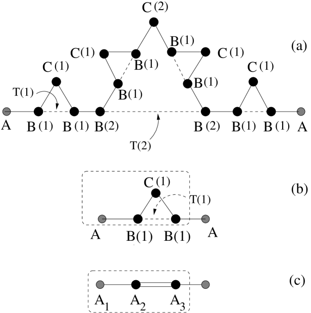
Figure 1: (a) A $2$nd generation Koch fractal with long range hopping. The sites $B(j)$ with $j=1$ and $2$ denote the ‘bulk sites’ where $j$ denotes the stage of hierarchy. Accordingly, the longer ranged hopping integrals are assigned values $T(j)$, $j=1$,$2$. The boundary sites are marked as $A$ and the remaining sites are $C$. (b) A unit cell (inside the dashed box) of a periodic approximant built by repeating a first generation Koch curve is shown. is enclosed in the dashed box, and, (c) The final trimer that is used for the trace analysis.

Exceptional results however, started surfacing in the last decade of the twentieth century, when it was shown by Dunlap et al dunlap that a certain kind of correlated disorder could lead to a finite number of resonant eigenstates in an otherwise disordered one dimensional (1-d) chain. Such states are extended but, of non-Bloch character, and lead to a ballistic transport of electrons at special values of the energy. The so called random dimer model (RDM) proposed by Dunlap et al dunlap led to a thorough investigation of the effect of correlated disorder on the electronic and other excitonic states in one dimensional systems  wu -lyra , where, ordinarily an un-correlated disorder renders all the states exponentially localized.

The effect of such short range correlations among the constituents in a one dimensional system has also led to exotic distribution of extended eigenstates in one dimensional quasi-periodic lattices arun1 -macia2 where, owing to the self similarity of such systems, one encounters an infinity of such extended states in an infinite 1-d system.

Deterministic fractals have also played their part. A subset of these structures has been shown to possess extended non-Bloch single particle states with a variety of transport properties wang1 -schwalm4 . In contrast to the RDM or the quasi-periodic chains in 1-d, the fractal lattices do not exhibit any short range clustering of atomic sites (in the sense of the RDM) that could possibly lead to local resonances resulting in a de-localization of the wave function. Rather, the topology of the entire lattice plays the key role in giving rise to such extended eigenstates at special values of energy of an electron hopping around in these lattices.

The extended states in the cases referred to, appear, in general, in isolation in the energy spectrum where they coexist with an otherwise singular continuous part. However, in recent times extensive numerical studies have pointed out towards a possibility of having a continuum of such extended states in a class of deterministic fractals arun3 -schwalm4 .

A universal feature of such extended states, whether they arise in RDM models or in the fractals reported so far is that, their existence is not sensitive to the numerical values of the Hamiltonian parameters. The short range clustering of the atomic sites or the overall lattice topology determined the criteria of the existence of unscattered eigenstates. In the present communication we report an exceptional case where, well defined correlations between the values of a subset of the Hamiltonian parameters is essential for the construction of an extended eigenstate which has equal amplitude at every lattice point. We explain the phenomenon by solving the Schrödinger equation on a Koch curve with hierarchical interaction maritan . A Koch curve with a long range hierarchical distribution of electron-hopping models, in an approximate manner, a polymeric system maritan . We show that this model can lead to unusual spectral and electronic transport properties when the hierarchy parameter is allowed to vary, mimicking (in a very crude sense though) local distortions in the system. The most astonishing result is that the same distribution of eigenstates, which makes the lattice conducting for a given set of the Hamiltonian parameters, represents a completely localized state with zero transmission across the Koch fractal. In addition to this, we find that such contrasting results are obtained for an infinite variety of values of the hierarchy parameter. These values are distributed in a self-similar manner, as is apparent from a study of the two-terminal transport across a Koch fractal. We work within a tight binding formalism and employ a real space renormalization group (RSRG) decimation scheme to unravel these strange states at all scales of length, and to obtain the end-to-end transmission properties of a Koch fractal of any size.

In what follows, we explain our work. In section II the model and the method are described. Section III contains the results and the discussion, and in section IV we draw our conclusion.

II The model and the method

We start by referring to Fig. 1.

Figure 2: Eigenvalue spectrum of a Koch fractal as a function of the hierarchical parameter $\lambda$ obtained from the trace of the transfer matrix for a $7$th generation fractal, taken as the ‘unit cell’.

The tight binding Hamiltonian in the Wannier basis reads,

$$H=\sum_{i}\epsilon_{i}c_{i}^{\dagger}c_{i}+\sum_{ij}t_{ij}c_{i}^{\dagger}c_{j}+h.c.$$ (1)

where, $\epsilon_{i}$ is the on-site energy of an electron at the site $i$. $t_{ij}$ is the hopping integral between neighboring sites. For nearest neighbor sites along the ridge of the Koch curve we assume $t_{ij}=t$, while the longer range hopping integrals can, in principle, take on any values. We shall illustrate our results for the specific case when the longer ranged hopping integrals assume values $T(n)=R^{n}t$, $R$ being the hierarchy parameter and $n$ represents the level of hierarchy. For a Koch fractal of finite but arbitrarily large size, the on-site potential $\epsilon_{i}$ will be assigned values $\epsilon_{A}$ (the extreme sites) and $\epsilon_{B}(n)$, $\epsilon_{C}(n)$ etc for the bulk sites depending on their positions in the lattice as explained in Fig. 1.

Owing to the self similarity of the lattice an application of the RSRG decimation method is used to scale the original system. An appropriate subset of sites are decimated leading to the recursion relations of the Hamiltonian parameters, viz,

$$\epsilon_{A}^{\prime} = \epsilon_{A}+\frac{(E-\xi)t^{2}}{\delta}$$

$$\epsilon_{B}(n)^{\prime} = \epsilon_{B}(n+1)+2\frac{(E-\xi)t^{2}}{\delta}$$

$$\epsilon_{C}(n)^{\prime} = \epsilon_{C}(n+1)+2\frac{(E-\xi)t^{2}}{\delta}$$

$$t^{\prime} = \frac{t^{2}\tilde{t}}{\delta}$$

$$T(n)^{\prime} = T(n+1)$$ (2)

where,

$$\xi = \epsilon_{B}(1)+\frac{t^{2}}{E-\epsilon_{C}(1)}$$

$$\tilde{t} = T(1)+\frac{t^{2}}{E-\epsilon_{C}(1)}$$

$$\delta = (E-\xi)^{2}-\tilde{t}^{2}$$ (3)

The above set of recursion relations will be used to extract information about the eigenvalue spectrum and to discern the nature of the eigenstates in the light of the motivation presented before.

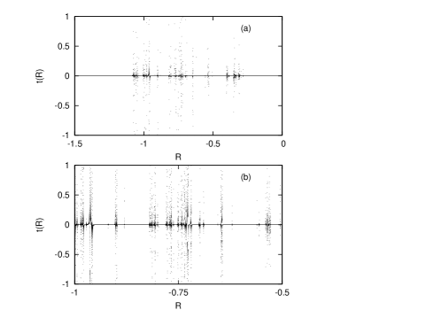
Figure 3: (a) Renormalized hopping between the extremities of a $9$th generation Koch fractal against the hierarchy parameter $R$ at an energy $E=\epsilon_{A}+t$. (b) A fine scan of the values of $R$ reveals the fractal nature of the distribution of the values of $R$.

III Results and discussion

III.1 The eigenvalue spectrum

We try to gain some insight into the spectrum of an infinite Koch fractal in the presence of hierarchically distributed long range interactions. To achieve this, we proceed in the spirit of the one dimensional quasi-periodic lattices koh -luck . The basic idea is to repeat a finite generation Koch curve periodically, pick up the unit cell and extract the energy values for which the trace of the transfer matrix for the unit cell remains bounded by two koh . A prototype unit cell for a periodic approximant generated by repeating the first generation Koch curve is shown in Fig. 1(b). To construct the transfer matrix and work out its trace in this case, the top vertex $C$ is decimated to reduce the system into a ‘triatomic molecule’ $A_{1}$-$A_{2}$-$A_{3}$ (Fig. 1(c)) where,

$$\epsilon_{A_{1}} = \epsilon_{A}$$

$$\epsilon_{A_{2}} = \epsilon_{B}(1)+\frac{t^{2}}{E-\epsilon_{C}(1)}$$ (4)

and, $\epsilon_{A_{3}}=\epsilon_{A_{2}}$. The ‘inter-atomic’ hopping integrals are $t_{{A_{1}}-{A_{2}}}=t$, and $t_{{A_{2}}-{A_{3}}}=T(1)+t^{2}/[E-\epsilon_{C}(1)]$. The transfer matrix across this triatomic molecule is then easily calculated. One can, in principle, begin with a fractal at any arbitrary generation, renormalize the parameters by sequentially applying the recursion relations Eq. 2 $n$-times, bring it down to an effective first generation block and subsequently to an effective triatomic molecule as discussed above to get the trace of the transfer matrix. The spectrum of an infinite lattice is obtained when the unit cell itself becomes infinitely large.

We present the result in Fig. 2 where the unit cell is a seventh generation Koch fractal with hierarchically distributed values of the long range hopping integrals $T(n)=R^{n}t$. The ‘band structure’ is displayed as the hierarchy parameter $R$ is varied. The behavior seems to saturate, at least becomes indistinguishable, for unit cells of larger size. So, the present figure can be taken to represent a very good approximation to the true eigenvalue spectrum in the infinite lattice limit.

With low absolute values of the hierarchy parameter $R$, the spectrum exhibits clustering of eigenvalues, giving rise to the formation of sub-bands. The sub-bands are separated by gaps which widen as $R$ increases. However, for $R$ quite large compared to the nearest neighbor hopping $t$, the sub-bands shrink in their widths and global gaps open up. An indefinite increase in the value of $R$ finds the spectrum consisting of a sparse distribution of points.

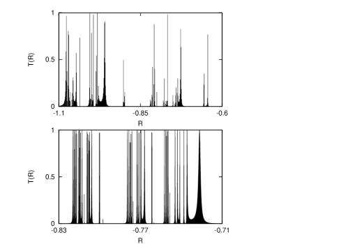
Figure 4: (a) The transmission coefficient of a $7$th generation Koch fractal with hierarchical interactions $-1\leq R\leq-0.6$, and (b) a finer scan for $-0.83\leq R\leq-0.71$. The fractal distribution of $T$ against $R$ is to be noted.

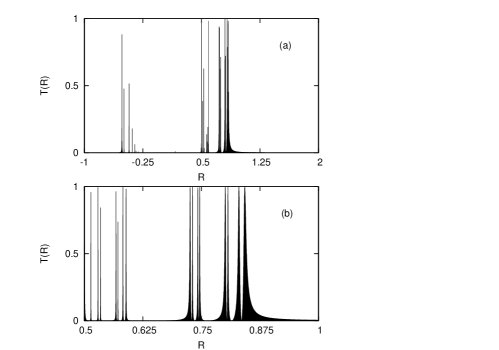
Figure 5: Transmission coefficient of a $6$th generation Koch fractal against the hierarchy parameter $R$. Here, the energy has been obtained from the equation $E=\epsilon_{A}^{\prime}+t^{\prime}$, that is, from a one step renormalized lattice. The variation with $R$ and its fine scan revealing again a self similar character, are shown in figures (a) and (b) respectively.

III.2 The atypically extended eigenstates

In this discussion we highlight certain aspects of a subset of eigenstates on a Koch fractal of finite but arbitrarily large generation. Let us choose the energy of the electron (the Fermi energy) as $E=\epsilon_{A}+t$. With this choice, it is easy to verify that one can construct an eigenstate whose amplitude at each site of the Koch fractal will be identical (normalized to unity, say) if we select

$$\epsilon_{C}(n) = \epsilon_{A}-t$$

$$\epsilon_{B}(n)+T(n) = \epsilon_{A}-t$$ (5)

for all $n\geq 1$. The above choices of the on-site potentials and the hierarchical hopping integrals $T(n)$ define a correlation between the values of the parameters of the Hamiltonian. Interestingly, we can see that once the on-site potential $\epsilon_{A}$ of the extreme sites and the nearest neighbor hopping matrix element $t$ are fixed, $\epsilon_{B}(n)$ and $T(n)$ can, in principle, be chosen from a set of random values, but in such a way, so as to satisfy the desired correlation, viz, $\epsilon_{B}(n)+T(n)=\epsilon_{A}-t$. Since, with this choice, the probability of finding the electron is same on every lattice point, it is not unusual to assume these states to be extended in the conventional language. However, a study of the flow of the nearest neighbor hopping integral $t$ under successive RSRG steps reveals a deeper story. It is known that, if, corresponding to certain value of the energy $E$, the hopping integral remains non-zero under RSRG iteration, it implies that the nearest neighbors are ‘connected’ at all scales of length. Hence, the corresponding eigenstate can legitimately be designated as an extended state. In the present case, the result of this investigation is found to be strongly sensitive to the initial choice of the parameters $\epsilon_{B}(n)$ and $T(n)$.

To clarify the above idea, we consider the particular situation where the longer range hopping integrals $T(n)$ are distributed in a hierarchical fashion, viz, $T(n)=R^{n}t$. We set $E=\epsilon_{A}+t$, and take $\epsilon_{C}(n)=\epsilon_{A}-t$ for all $n$. The choice of $\epsilon_{B}(n)$ is then restricted by the desired correlation as it appears in the last of the equations in Eq. 5. A Koch fractal, on successive renormalization by an appropriate number of steps may be reduced to an effective diatomic molecule comprising of the end sites only. The effective hopping between the surviving end sites will decide on the extendedness of the wave function at that particular energy. Most interestingly we find that, the flow of the hopping integral $t$ under successive iterations is strongly sensitive to the choice of the hierarchy parameter $R$ (which automatically fixes $\epsilon_{B}(n)$). We present one such result in Fig. 3, where the end-to-end renormalized hopping in a $9$th generation Koch fractal is plotted as a function of the hierarchy parameter $R$. We have taken $E=1$ and $T(n)=R^{n}t$ with $\epsilon_{A}=0$, $t=1$, $\epsilon_{C}(n)=-1$ (for all $n$), and $\epsilon_{B}(n)=\epsilon_{A}-t-T(n)$. It must be appreciated that for every value of $R$, with the above conditions being satisfied, the wave function displays an identical pattern of amplitudes on all sites. yet, we find that the end-to-end hopping becomes zero or remains finite depending on the values of $R$ (and hence the values of $\epsilon_{B}(n)$). In addition to that, a finer scan of any of the intervals of $R$ reveals that the values of the hierarchy parameter for which the end-to-end hopping across a Koch fractal of any generation remains non-zero (a true extended state), are distributed in a self-similar, fractal pattern. Every value of $R$, defines a new point in the parameter space $[\epsilon_{A},\epsilon_{B}(n),\epsilon_{C}(n),T(n),t]$. therefore, for $E=\epsilon_{A}+t$, we come across a fractal distribution of points in the parameter space. The features described above are reflected in the end-to-end transmission across a finite Koch curve with hierarchical interactions. The results are presented below.

III.3 The transmission coefficient

We have examined the two-terminal transport of a Koch fractal of an arbitrary generation by placing the lattice between two semi-infinite perfectly periodic leads characterized by a constant on-site potential $\epsilon_{0}$ and nearest neighbor hopping integral $t_{0}$. A $k$-th generation fractal is reduced, by applying the decimation recursion relations Eq. 2 $k$ times, to an effective diatomic molecule comprising of the extreme sites $A-A$ with renormalized on-site potential $\epsilon_{A}^{(k)}$ and renormalized ‘inter atomic’ hopping integral $t^{(k)}$. The transmission coefficient $\tau$ is then obtained from the well known formula stone ,

$$\tau=\frac{4\sin^{2}qa}{[M_{12}-M_{21}+(M_{11}-M_{22})\cos qa]^{2}+[M_{11}+M_{22}]^{2}\sin^{2}qa}$$ (6)

Here,

$$M_{11} = \frac{[E-\epsilon_{A}^{(k)}]^{2}}{t_{0}t^{(k)}}-\frac{t^{(k)}}{t_{0}}$$

$$M_{12} = -\frac{E-\epsilon_{A}^{(k)}}{t^{(k)}}$$

$$M_{21} = -M_{12}$$

$$M_{22} = -\frac{t_{0}}{t^{(k)}}$$ (7)

The lattice spacing $a$ in the leads is taken to be unity, and $q=\cos^{-1}[(E-\epsilon_{0})/(2t_{0})]$. Throughout the calculations we take $\epsilon_{0}=0$ and $t_{0}=1$.

Fig. 4 (a) displays the transmission across a $7$th generation fractal for $E=\epsilon_{A}+t$ for a certain choice of the range of the hierarchy parameter $R$. For every value of $R$ in this range, we have taken $\epsilon_{B}(n)=\epsilon_{A}-t-T(n)$ which makes the amplitudes of the wave function same at every site (normalized to one). The spectrum consists of gaps and resonant transmissions indicating that, for certain values of $R$ the $7$th generation Koch network may become completely transparent to an incoming electron with the above energy, while that same electron finds the network totally opaque for other values of $R$. A fine scan of a sub-interval of $R$ reveals that the values of $R$ presenting the above feature are indeed distributed in a self-similar, fractal manner. This is illustrated in Fig. 4(b) and is in agreement with the initial observations made based on the recursive behavior of the nearest neighbor hopping.

One can construct eigenstates for which the amplitudes will be same (unity) at all the sites of a renormalized Koch fractal as well. The procedure outlined above for the lattice at the bare length scale is to be implemented on a renormalized version of the system. For example, we can set $E=\epsilon_{A}^{\prime}+t^{\prime}$ on a one step renormalized lattice. The eigenvalues of the desired states are then extracted by solving the polynomial equation

$$E-F\left(\epsilon_{A},t,\epsilon_{B}(1),\epsilon_{C}(1),T(1)\right)=0$$ (8)

where,

$$F=\frac{\epsilon_{A}E^{2}+E\left[t^{2}-\epsilon_{A}\left(\epsilon_{B}(1)+\epsilon_{C}(1)+T(1)\right)\right]+\epsilon_{A}\left[\epsilon_{B}(1)\epsilon_{C}(1)-2t^{2}+\epsilon_{C}(1)T(1)\right]-t^{2}\epsilon_{C}(1)}{E^{2}-\left[\epsilon_{B}(1)+\epsilon_{C}(1)+T(1)\right]E+\epsilon_{B}(1)\epsilon_{C}(1)-2t^{2}+\epsilon_{C}(1)T(1)}$$ (9)

The potentials and the hopping integrals appearing as the arguments of $F$ can be chosen independently. It is to be appreciated that the roots of the equations are free from $\epsilon_{B}(n)$ and $\epsilon_{C}(n)$ and $T(n)$ for $n\geq 2$. We shall now demand $\epsilon_{C}(1)^{\prime}=\epsilon_{A}^{\prime}-t^{\prime}$ which leads to an equation defining $\epsilon_{C}(2)$ in the original lattice, viz,

$$\epsilon_{C}(2)=\left[\epsilon_{A}^{\prime}-t^{\prime}-\Delta\right]_{E=\epsilon_{A}^{\prime}+t^{\prime}}$$ (10)

where,

$$\Delta=\frac{t^{2}}{E+T(1)-\epsilon_{B}(1)}+\frac{[E-\epsilon_{C}(1)]t^{2}}{E^{2}-E[\epsilon_{C}(1)+T(1)]+\epsilon_{C}(1)[\epsilon_{B}(1)+T(1)]-2t^{2}}$$ (11)

The energy $E$ is chosen from the solutions of Eq. 8. This settles the initial value of $\epsilon_{C}(2)$ we should begin with. To mimic the earlier situation in the original scheme (the bare length scale) we now set $\epsilon_{C}(n)=\epsilon_{C}(2)$, as obtained above, for all $n\geq 2$ in the original Koch geometry..

In addition to this, we should set $\epsilon_{B}(n)^{\prime}+T(n)^{\prime}=\epsilon_{A}^{\prime}-t^{\prime}$ for $n\geq 1$, which leads to the selection of the un-primed values of $\epsilon_{B}(n)$ and $T(n)$ such that, $\epsilon_{B}(n)+T(n)=(\epsilon_{A}^{\prime}-t^{\prime}-\Delta)_{E=\epsilon_{A}^{\prime}+t^{\prime}}=\epsilon_{C}(2)$, for $n\geq 2$ on the original (bare length scale) lattice. The entire scheme now works just as it worked in the original scale of length. The process can, in principle, go on and every time we extract the energy eigenvalue by solving the polynomial equation $E-\epsilon_{A}^{(k)}-t^{(k)}=0$ from the $k-$th stage of renormalization, we need to pre-define a bigger parameter space to begin with. The energy of course remains independent of $\epsilon_{B}(n)$, $\epsilon_{C}(n)$ or $T(n)$ for $n>k$. The scheme works, the correlations become much more complicated though.

IV Conclusion

In conclusion, we have unraveled a set of atypical extended states in Koch fractals possessing hierarchically long range interactions. The states have identical amplitudes at all atomic sites in the lattice for mutually correlated values of a certain set of the Hamiltonian parameters. The same distribution of amplitudes on a Koch curve of arbitrary generation may represent either a completely transparent state or a strictly localized one depending on the choice of the parameters. This fact has been illustrated by choosing the long range hopping integrals to be distributed in a hierarchical, but deterministic fashion, and by tuning the hierarchical parameter appropriately and according to the terms dictated by the correlation.

ACKNOWLEDGMENT

I thank Enrique Maciá for an early discussion on this work, and Bibhas Bhattacharyya for helpful suggestions.

References

- (1) P. W. Anderson, Phys. Rev. 109, 1492 (1958); E. Abrahams, P. W. Anderson, D. C. Liciardello, and T. V. Ramakrishnan, Phys. Rev. Lett. 42, 673 (1979).
- (2) F. Guinea, and J. A. Vergés, Phys. Rev. B 35, 979 (1987).
- (3) M. Hjort and S. Stafström, Phys. Rev. B 62, 5245 (2000).
- (4) M. Kohmoto, L. P. Kadanoff, and C. Tang, Phys. Rev. Lett. 50, 1870 (1983).
- (5) J. Bellissard, A. Bovier, and J. M. Ghez, Commun. Math. Phys. 135, 379 (1991).
- (6) Y. Liu and R. Riklund, Phys. Rev. B 35, 6034 (1987).
- (7) J. B. Sokoloff, Phys. Rep. 126, 189 (1985).
- (8) J. M. Luck, Phys. Rev. B 39, 5834 (1989).
- (9) E. Domany, S. Alexander, D. Bensimon, and L. P. Kadanoff, Phys. Rev. 28, 3110 (1982).
- (10) R. Rammal and G. Toulose, Phys. Rev. Lett. 49, 1194 (1982).
- (11) J. R. Banavar, L. Kadanoff, and A. M. M. Pruisken,
- (12) Ho-Fai Chung, E. K. Riedel, and Y. Gefen, Phys. Rev. Lett. 62, 587 (1989).
- (13) Ho-Fai Chung and E. K. Riedel, Phys. Rev. B 40, 9498 (1989).
- (14) W. A. Schwalm and M. K. Schwalm, Phys. Rev. B 39, 12872 (1989).
- (15) R. F. S. Andrade H. J. Schellnhuber, Europhys. Lett. 10, 73 (1989).
- (16) W. A. Schwalm and M. K. Schwalm, Phys. Rev. B 44, 382 (1991).
- (17) R. F. S. Andrade and H. J Schellnhuber, Phys. Rev. B 44, 13213 (1991).
- (18) W. A. Schwalm and M. K. Schwalm, Phys. Rev. B 47, 7847 (1993).
- (19) D. H. Dunlap, H. L. Wu, and P. Phillips, Phys. Rev. Lett. 65, 88 (1990).
- (20) H. L. Wu and P. Phillips, J. Chem. Phys. 93, 7369 (1990); Phys. Rev. Lett. 66, 1366 (1991).
- (21) P. K. Dutta, D. Giri, and K. Kundu, Phys. Rev. B 47, 10727 (1993).
- (22) E. Diez, A. Sanchez, F. Dominguez-Adame, and G. P. Berman, Phys. Rev. B 54, 14550 (1996).
- (23) F. Dominguez-Adame, A. Sanchez, and E. Diez, Phys. Rev. B 50, 17336 (1994); J. Appl. Phys. 81, 77 (1997).
- (24) M. Hilke and J. C. Flores, Phys. Rev. B 55, 10625 (1997).
- (25) A. Brezini, P. Fulde, and M. Dairi, Int. J. Mod. Phys. B 23, 4987 (2009).
- (26) F. A. B. F. de Moura and M. L. Lyra, Phys. Rev. Lett. 81, 3735 (1998).
- (27) F. A. B. F. de Moura, M. D. Coutinho-Filho, E. P. Raposo, and M. L. Lyra, Phys. Rev. B 66, 014418 (2002); ibid 68, 012202 (2003).
- (28) A. Chakrabarti, S. N. Karmakar, and R. K. Moitra, Phys. Rev. B 49, 9503 (1994).
- (29) A. Chakrabarti, S. N. Karmakar, and R. K. Moitra, Phys. Rev. Lett. 76, 2957 (1996).
- (30) E. Maciá and F. Dominguez-Adame, Electrons, Phonons and Excitons in Low Dimensional Aperiodic Systems, Editorial Complutense, Madrid (2000).
- (31) E. Maciá and F. Dominguez-Adame, Phys. Rev. Lett. 76, 2957 (1996).
- (32) X. R. Wang, Phys. Rev. B 51, 9310 (1994).
- (33) X. R. Wang, Phys. Rev. B 53, 12035 (1996).
- (34) A. Chakrabarti, Phys. Rev. B 60, 10576 (1999).
- (35) A. Chakrabarti, Phys. Rev. B 72, 134207 (2005).
- (36) E. Maciá, Phys. Rev. B 57, 7661 (1998).
- (37) W. Schwalm and B. J. Moritz, Phys. Rev. B 71, 134207 (2005).
- (38) A. Maritan and A. Stella, Phys. Rev. B 34, 456 (1986).
- (39) P. Kappertz, R. F. S. Andrade, and H. J Schellnhuber, Phys. Rev. B 49, 14711 (1994).
- (40) R. F. S. Andrade and H. J Schellnhuber , Phys. Rev. B 55, 12956 (1996).
- (41) R. F. S. Andrade and H. J Schellnhuber, Phys. Rev. B 55, 12956 (1997).
- (42) A. Douglas Stone, J. D. Joannopoulos, and D. J. Chadi, Phys. Rev. B 24, 5583 (1981).