Optical vortices of slow light using tripod scheme

Abstract

We consider propagation, storing and retrieval of slow light (probe beam) in a resonant atomic medium illuminated by two control laser beams of larger intensity. The probe and two control beams act on atoms in a tripod configuration of the light-matter coupling. The first control beam is allowed to have an orbital angular momentum (OAM). Application of the second vortex-free control laser ensures the adiabatic (lossles) propagation of the probe beam at the vortex core where the intensity of the first control laser goes to zero. Storing and release of the probe beam is accomplished by switching off and on the control laser beams leading to the transfer of the optical vortex from the first control beam to the regenerated probe field. A part of the stored probe beam remains frozen in the medium in the form of atomic spin excitations, the number of which increases with increasing the intensity of the second control laser. We analyse such losses in the regenerated probe beam and provide conditions for the optical vortex of the control beam to be transferred efficiently to the restored probe beam.

Keywords: slow light, electromagnetically induced transparency, light storage, orbital angular momentum

1 Introduction

Over the last decade there has been a great deal of activities in slow [1, 2, 3, 4, 5], stored [6, 7, 8, 9, 10, 11, 12, 13, 14, 15, 16, 17, 18] and stationary [19, 20, 21, 22, 23, 24, 25] light. It was demonstated that a resonant weak pulse of light (to be referred to as the probe light) can propagate as slow as several of tens of meters per second [1] in an atomic medium driven by a stronger (control) laser beam. The application of the control laser beam makes the resonant and opaque medium transparent for the probe beam due the electromagnetically induced transparence (EIT) [26, 27, 28, 29, 30], both beams making a $\Lambda$ configuration of the atom-light coupling. The EIT can be used not only to slow down dramatically the light pulses [1, 2, 3, 4, 5], but also to store them [7, 8, 13, 15, 16, 17, 18] in atomic gases. The storage and release of the probe pulses has been accomplished [7, 8, 13, 15, 16, 17, 18] by switching off and on the control laser [6]. The slow and storred light can be applied to reversible quantum memories [6, 9, 10, 13, 29, 30, 31, 32, 33] and, in the case of moving media [34, 35, 36, 37, 38, 39, 40, 41], also to rotational sensing devices.

The orbital angular momentum (OAM) [42, 43] provides additional possibilities in manipulating the slow light. The optical OAM represents a new degree of freedom which can be exploited in the quantum computation and quantum information storage [43]. Most of the previous studies on the vortex slow light have concentrated on situations in which the incident probe beam carries an OAM [44, 45, 41, 46, 47].

Here we consider another situation in which the incident probe beam does not have an optical vortex, yet it gains the OAM when retrieved. For this purpose one of the control laser beam is assumed to have an optical vortex during either the storage or retrieval of the slow light. The intensity of such a control beam goes to zero at the vortex core, potentially leading to the absorption losses of the probe beam in this area. To avoid the losses an extra control laser without an optical vortex is used. This makes a more complex tripod scheme of the atom-light coupling [48, 49, 50, 51, 52, 53, 54, 55, 56, 57, 58, 59]. The total intensity of the control lasers is then non-zero at the vortex core of the first control laser preventing the absorption losses. Subsequently we analyze additional losses appearing because a part of the stored probe beam remains frozen in the atomic cloud in the form of spin excitations during the exchange of the optical vortex between the control laser and the regenerated slow light. A number of such frozen excitations increases with increasing the intensity of the second control laser. We provide conditions for the optical vortex of the control beam to be transferred efficiently to the restored probe beam.

2 Equations for the probe beam

In this Section we shall derive general equations for the propagation of the probe beam in an ensemble of tripod atoms. In doing so we shall not make use of the usual slowly-varying amplitude approximation [55, 57, 56] for the spatial coordinates in the direction perpendicular to the light propagation. This will make it possible to analyse situations where the control and/or probe beams have the OAM.

2.1 Coupled equations for the probe beam and atoms

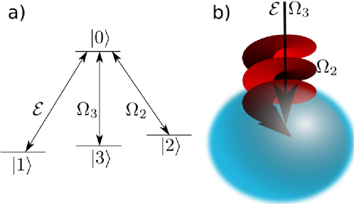
Figure 1: Light induced transitions in the cloud of cold atoms involving a tripod configuration of the internal atomic states.

Let us consider an ensemble of tripod-type atoms characterised by three hyperfine ground levels $1$, $2$, and $3$, as well as an electronic excited level $0$ (figure 1). The translational motion of atoms is represented by a four component column operator $\Psi(\bi{r})$, where the components $\Psi_{1}(\bi{r},t)$, $\Psi_{2}(\bi{r},t)$, $\Psi_{3}(\bi{r},t)$, and $\Psi_{0}(\bi{r},t)$ are the field operators describing to the center of mass motion in the four internal atomic states. The quantum nature of the atoms comprising the medium will determine whether these field operators obey Bose-Einstein or Fermi-Dirac commutation relations. The atoms interact with three light fields in a tripod configuration of the atom-light coupling [48, 53, 55, 56, 57]. Specifically, two strong classical control lasers induce transitions $|2\rangle\rightarrow|0\rangle$, $|3\rangle\rightarrow|0\rangle$ and a weaker quantum probe field drives a transition $|1\rangle\rightarrow|0\rangle$, as shown in figure 1.

The electric field of the probe beam is

$$\bi{E}(\bi{r},t)=\hat{\bi{e}}\sqrt{\frac{\hbar\omega}{2\varepsilon_{0}}}\mathcal{E}(\bi{r},t)\rme^{-\rmi\omega t}+\mathrm{H.c.}\,,$$ (1)

where $\omega=ck$ is the central frequency of the probe photons, $\bi{k}=\hat{\bi{z}}k$ is the wave vector, and $\hat{\bi{e}}\bot\hat{\bi{z}}$ is the unit polarization vector. This field can be considered to be either a quantum operator or a classical variable. We have chosen the dimensions of the electric field amplitude $\mathcal{E}$ to be such that its squared modulus represents the number density of probe photons. The probe field is assumed to be quasi-monochromatic, so the amplitude $\mathcal{E}(\bi{r},t)$ changes little over the time of an optical cycle and thus obeys the following equation:

$$\left(\partial_{t}-\rmi\frac{c^{2}}{2\omega}\nabla^{2}-\rmi\frac{\omega}{2}\right)\mathcal{E}=\rmi g\Phi_{1}^{{\dagger}}\Phi_{0}\,,$$ (2)

where have introduce the slowly varying atomic field operators $\Phi_{1}=\Psi_{1}\rme^{\rmi\omega_{1}t}$, $\Phi_{2}=\Psi_{2}\rme^{\rmi(\omega_{1}+\omega-\omega_{c2})t}$, $\Phi_{3}=\Psi_{3}\rme^{\rmi(\omega_{1}+\omega-\omega_{c3})t}$, $\Phi_{0}=\Psi_{0}\rme^{\rmi(\omega_{1}+\omega)t}$, with $\hbar\omega_{1}$ being the energy of the atomic ground state $1$, $\omega_{c2}$ and $\omega_{c3}$ being the frequencies of the control fields. The parameter $g=\mu\sqrt{\omega/2\varepsilon_{0}\hbar}$ featured in equation (2) characterizes the strength of coupling of the probe field with the atoms , $\mu$ being the dipole moment of the atomic transition $|1\rangle\rightarrow|0\rangle$. Note that, unlike in the usual treatment of slow light, we have retained the second-order derivative $\nabla^{2}$ in the equation of motion (2). This allows one to account for the fast changes of $\mathcal{E}$ in a direction perpendicular to the wave vector $\bi{k}$, i.e., in the $xy$ plane. Therefore our analysis can be applied to the twisted beams of light $\mathcal{E}(\bi{r},t)\sim\exp(\rmi l\varphi)$ carrying an OAM $\hbar l$ per photon.

In the following we shall make use of a semi-classical picture in which both the electromagnetic and matter field operators are replaced by $c$ numbers. The equations for the matter fields are then

$$\rmi\partial_{t}\Phi_{1}=-g\mathcal{E}^{*}\Phi_{0}$$ (3)

$$\rmi\partial_{t}\Phi_{0}=(\omega_{01}-\rmi\gamma)\Phi_{0}-\Omega_{\mathrm{c}2}\Phi_{2}-\Omega_{\mathrm{c}3}\Phi_{3}-g\mathcal{E}\Phi_{1}$$ (4)

$$\rmi\partial_{t}\Phi_{2}=\omega_{21}\Phi_{2}-\Omega_{\mathrm{c}2}^{*}\Phi_{0}$$ (5)

$$\rmi\partial_{t}\Phi_{3}=\omega_{31}\Phi_{3}-\Omega_{\mathrm{c}3}^{*}\Phi_{0}\,,$$ (6)

Here $\Omega_{\mathrm{c}2}$ and $\Omega_{\mathrm{c}3}$ are the Rabi frequencies of control lasers driving the transitions $|2\rangle\rightarrow|0\rangle$ and $|3\rangle\rightarrow|0\rangle$; $\gamma$ is the decay rate of the excited level; $\omega_{21}=\omega_{2}-\omega_{1}+\omega_{c2}-\omega$ and $\omega_{31}=\omega_{3}-\omega_{1}+\omega_{c3}-\omega$ are frequencies of the electronic detuning from the two-photon resonances, $\omega_{01}=\omega_{0}-\omega_{1}-\omega$ is the frequency of the electronic detuning from the one-photon resonance. In writing equations (3)–(6) we used the rotating wave approximation for the atom-light coupling, and neglected the terms containing atomic mass $m$, since from now on we are not interested in the effects due to the atomic motion: The terms containing atomic mass $m$ would be important in equations (3)–(6) for the description of the light-dragging effects [36, 37, 39, 40, 41]. Furthermore we assumed that the trapping potentials for an atom in the electronic state $j$ ($j=1,2,3,0$) are position independent and hence can be omitted.

2.2 Equation for the of probe beam

To analyze the atomic dynamics it is convenient to introduce the bright and dark states of the atomic center of mass motion

$$\Phi_{\mathrm{B}}=\Omega_{\mathrm{c}}^{-1}(\Omega_{\mathrm{c}2}\Phi_{2}+\Omega_{\mathrm{c}3}\Phi_{3})\,,$$ (7)

$$\Phi_{\mathrm{D}}=\Omega_{\mathrm{c}}^{-1}(\Omega_{\mathrm{c}3}^{*}\Phi_{2}-\Omega_{\mathrm{c}2}^{*}\Phi_{3})\,,$$ (8)

where

$$\Omega_{\mathrm{c}}=\sqrt{|\Omega_{\mathrm{c}2}|^{2}+|\Omega_{\mathrm{c}3}|^{2}}$$ (9)

is the total Rabi frequency. It is the wave-function $\Phi_{\mathrm{B}}$ which is featured in the equation of motion (4) for the excited state wave-function. On the other hand, the dark state is not coupled directly to the excited level $0$. The original fields $\Phi_{2}$ and $\Phi_{3}$ can be expressed through $\Phi_{\mathrm{B}}$ and $\Phi_{\mathrm{D}}$ as

$$\Phi_{2}=\Omega_{\mathrm{c}}^{-1}(\Omega_{\mathrm{c}2}^{*}\Phi_{B}+\Omega_{\mathrm{c}3}\Phi_{D})\,,$$ (10)

$$\Phi_{3}=\Omega_{\mathrm{c}}^{-1}(\Omega_{\mathrm{c}3}^{*}\Phi_{B}-\Omega_{\mathrm{c}2}\Phi_{D})\,.$$ (11)

Initially the atoms are in the ground level $1$ and the Rabi frequency of the probe field is considered to be much smaller than $\Omega_{\mathrm{c}}$. Consequently one can neglect the last term in equation (3) that causes depletion of the ground level $1$, giving $i\partial_{t}\Phi_{1}=0$. If the atoms in the internal ground-state $1$ form a BEC, its wave function $\Phi_{1}=\sqrt{n}\exp(iS_{1})$ represents an incident variable determined by the atomic density $n$ and the condensate phase $S_{1}$. The latter phase will not play an important role in our subsequent analysis, since we are not interested in the effects due to the condensate dynamics.

Suppose the control and probe beams are tuned close to the two-photon resonance. Application of such laser beams cause electromagnetically induced transparency (EIT) in which the transitions $|2\rangle\rightarrow|0\rangle$, $|3\rangle\rightarrow|0\rangle$, and $|1\rangle\rightarrow|0\rangle$ interfere destructively preventing population of the excited state $0$. The adiabatic approximation is obtained neglecting the excited state population in equation (4), giving

$$\Phi_{\mathrm{B}}=-g\frac{\Phi_{1}}{\Omega_{\mathrm{c}}}\mathcal{E}\,.$$ (12)

When the adiabatic approximation is valid, the bright and dark states are coupled weakly. Therefore, combining equations (5)), (6) and neglecting the dark state contribution $\Phi_{D}$, we arrive at the equation for the bright state wave-function

$$\rmi\partial_{t}\Phi_{\mathrm{B}}=\delta\Phi_{\mathrm{B}}-\Omega_{\mathrm{c}}\Phi_{0}\,,$$ (13)

where

$$\delta=\omega_{21}|\xi_{2}|^{2}+\omega_{31}|\xi_{3}|^{2}-\rmi(\xi_{2}\partial_{t}\xi_{2}^{*}+\xi_{3}\partial_{t}\xi_{3}^{*})$$ (14)

is the two-photon frequency mismatch, with

$$\xi_{2}=\Omega_{\mathrm{c}2}/\Omega_{\mathrm{c}}\,,\qquad\xi_{3}=\Omega_{\mathrm{c}3}/\Omega_{\mathrm{c}}\,.$$ (15)

The derivation of equation (13) can be found in more details in our earlier work [60] on the light-induced gauge potentials for the $\Lambda$ type atoms. Equation (13) relates $\Phi_{0}$ to the bright state $\Phi_{\mathrm{B}}$ as

$$\Phi_{0}=\Omega_{\mathrm{c}}^{-1}(-\rmi\partial_{t}+\delta)\Phi_{\mathrm{B}}\,.$$ (16)

Finally, equations (2), (12) and (16) provide a closed equation for the electric field amplitude $\mathcal{E}$:

$$\left(\partial_{t}-\rmi\frac{c^{2}}{2\omega}\nabla^{2}-\rmi\frac{\omega}{2}\right)\mathcal{E}=-\rmi\frac{g^{2}\Phi_{1}^{*}}{\Omega_{\mathrm{c}}}(-\rmi\partial_{t}+\delta)\frac{\Phi_{1}}{\Omega_{\mathrm{c}}}\mathcal{E}\,.$$ (17)

This equation applies a wide variety of phenomena. In particular it can be used to model light storage by introducing time dependence in $\Omega_{\mathrm{c}}$ or light dragging due to spatial variation of $\Omega_{\mathrm{c}}$ or $\Phi_{1}$.

2.3 Non-adiabatic corrections

In the next Section we shall consider the releasing of the stored light. For this we should include non-adiabatic corrections to the equation of motion (17). This can be done in the following way. From equation (4) expressing the bright state $\Phi_{\mathrm{B}}$ and substituting equation (16) for $\Phi_{0}$ we get

$$\Phi_{\mathrm{B}}=-\frac{g\mathcal{E}}{\Omega_{\mathrm{c}}}\Phi_{1}+\Omega_{\mathrm{c}}^{-1}(-\rmi\partial_{t}+\omega_{01}-\rmi\gamma)\Omega_{\mathrm{c}}^{-1}(-\rmi\partial_{t}+\delta)\Phi_{\mathrm{B}}\,.$$ (18)

The term with the decay rate $\gamma$ is larger than other non-adiabatic corrections in the above equation. Keeping in the non-adiabatic corrections only the terms proportional to the decay rate $\gamma$ and neglecting, for simplicity, the two-photon detuning $\delta$ we obtain

$$\Phi_{\mathrm{B}}\approx-\frac{g\mathcal{E}}{\Omega_{\mathrm{c}}}\Phi_{1}-\frac{\gamma}{\Omega_{\mathrm{c}}^{2}}\partial_{t}\Phi_{\mathrm{B}}\,.$$ (19)

The solution of this equation, assuming that the control beam is switched on suddenly at $t=0$ an then changes slowly during the characteristic relaxation time $\gamma/\Omega_{\mathrm{c}}^{2}$, is

$$\Phi_{\mathrm{B}}=\Phi_{\mathrm{B}}(0)\rme^{-\frac{\Omega_{c}^{2}}{\gamma}t}-\frac{g\mathcal{E}}{\Omega_{\mathrm{c}}}\Phi_{1}\left(1-\rme^{-\frac{\Omega_{\mathrm{c}}^{2}}{\gamma}t}\right)\,.$$ (20)

Using equations (16) and (20), the equation for the electric field (2) takes the form

$$\left(\partial_{t}-\rmi\frac{c^{2}}{2\omega}\nabla^{2}-\rmi\frac{\omega}{2}\right)\mathcal{E}=-\rmi\frac{g^{2}\Phi_{1}^{*}}{\Omega_{\mathrm{c}}}(-\rmi\partial_{t}+\delta)\frac{\Phi_{1}}{\Omega_{\mathrm{c}}}\mathcal{E}\left(1-\rme^{-\frac{\Omega_{\mathrm{c}}^{2}}{\gamma}t}\right)$$

$$+\rmi\frac{g\Phi_{1}^{*}}{\Omega_{\mathrm{c}}}(-\rmi\partial_{t}+\delta)\Phi_{\mathrm{B}}(0)\rme^{-\frac{\Omega_{\mathrm{c}}^{2}}{\gamma}t}\,.$$ (21)

At $t=0$ the probe field is off, and the information on the previously stored probe beam being contained in the atomic coherence $\Phi_{\mathrm{B}}(0)$. The regeneration of the probe beam is described by the second term on the r.h.s. of equation (21) representing the source for the electric field. Retaining only the temporal derivatives in equation (21), we get the equation describing the generation of the electric field:

$$\left[1+\frac{g^{2}n}{\Omega_{\mathrm{c}}^{2}}\left(1-\rme^{-\frac{\Omega_{\mathrm{c}}^{2}}{\gamma}t}\right)\right]\partial_{t}\mathcal{E}=-\frac{g\Phi_{1}^{*}}{\gamma}[g\Phi_{1}\mathcal{E}+\Omega_{\mathrm{c}}\Phi_{\mathrm{B}}(0)]\rme^{-\frac{\Omega_{\mathrm{c}}^{2}}{\gamma}t}\,,$$ (22)

with the initial condition $\mathcal{E}(0)=0$ at $t=0$. For time in access of the relaxation time $\gamma/\Omega_{\mathrm{c}}^{2}$ the regenerated probe field evolves to a steady-state value complying with the adiabatic condition (12)

$$\mathcal{E}=-\frac{\Omega_{\mathrm{c}}}{g\Phi_{1}}\Phi_{\mathrm{B}}(0)\,.$$ (23)

In this way, the regenerated electric field $\mathcal{E}$ is indeed determined by the initial atomic coherence $\Phi_{\mathrm{B}}(0)$. The subsequent evolution of the probe field is described by the adiabatic equation of motion (17) containing both the temporal and spatial derivatives subject to the initial condition (23).

2.4 Co-propagating control and probe beams

Suppose the probe and control beams co-propagate: $\mathcal{E}(\bi{r},t)=\tilde{\mathcal{E}}(\bi{r},t)\rme^{\rmi kz}$, $\Omega_{\mathrm{c}2}(\bi{r},t)=\Omega_{2}(\bi{r},t)\rme^{\rmi k_{\mathrm{c}2}z}$, $\Omega_{\mathrm{c}3}(\bi{r},t)=\Omega_{3}(\bi{r},t)\rme^{\rmi k_{\mathrm{c}3}z}$, where $k_{\mathrm{c}2}$ and $k_{\mathrm{c}3}$ are the wave numbers of the control beams. For paraxial beams the amplitudes $\tilde{\mathcal{E}}(\bi{r},t)$, $\Omega_{2}(\bi{r},t)$ and $\Omega_{3}(\bi{r},t)$ depend weakly in the propagation direction $z$ compared to the variation of the exponential factors. Equation (17) for the probe field takes then the form

$$\partial_{t}\tilde{\mathcal{E}}+v_{\mathrm{g}}\left[\frac{\partial}{\partial z}+\left(\frac{1}{v_{\mathrm{g}}}-\frac{1}{c}\right)\rmi\delta-\rmi\frac{1}{2k}\nabla_{\bot}^{2}\right]\tilde{\mathcal{E}}=\left(1-\frac{v_{\mathrm{g}}}{c}\right)\frac{\partial_{t}\Omega_{{\mathrm{c}}}}{\Omega_{{\mathrm{c}}}}\tilde{\mathcal{E}}\,,$$ (24)

where we have replaced $\nabla^{2}$ by its transverse part $\nabla_{\bot}^{2}=\partial^{2}/\partial x^{2}+\partial^{2}/\partial y^{2}$ because of the paraxial approximation. Here

$$v_{\mathrm{g}}=c\left(1+\frac{g^{2}n}{\Omega_{\mathrm{c}}^{2}}\right)^{-1}$$ (25)

is the radiative group velocity. The term with spatial derivative $\partial/\partial z$ in equation (24) describes the radiative propagation along the $z$ axis with the group velocity $v_{\mathrm{g}}$.

3 Storing and releasing the light

The probe beam $\mathcal{E}^{(\mathrm{s})}$ enters an atomic medium which is illuminated by two control beams characterized by the Rabi frequencies $\Omega_{\mathrm{c}2}^{(\mathrm{s})}$ and $\Omega_{\mathrm{c}3}^{(\mathrm{s})}$, where the index $(\mathrm{s})$ refer to the stage of storing the light. At the boundary the probe beam is converted into a polariton propagating slowly in the medium with the velocity $v_{\mathrm{g}}^{(\mathrm{s})}\ll c$. At certain time $t=t^{(\mathrm{s})}$ the whole probe pulse enters the atomic medium and is contained in it. Since the atomic population is created exclusively by the incident light field, the atomic dark-state $\Phi_{\mathrm{D}}$ is not populated and, according to equation (12), the bright-state is

$$\Phi_{\mathrm{B}}^{(\mathrm{s})}(t^{(\mathrm{s})})=-g\frac{\Phi_{1}}{\Omega_{\mathrm{c}}^{(\mathrm{s})}}\mathcal{E}^{(\mathrm{s})}(t^{(\mathrm{s})})\,.$$ (26)

Equations (10) and (11) give the atomic fields:

$$\Phi_{2}^{(\mathrm{s})}=\xi_{\mathrm{c}2}^{(\mathrm{s})*}\Phi_{\mathrm{B}}^{(\mathrm{s})}\,,\qquad\Phi_{3}^{(\mathrm{s})}=\xi_{\mathrm{c}3}^{(\mathrm{s})*}\Phi_{\mathrm{B}}^{(\mathrm{s})}\,.$$ (27)

To store the slow light, both control fields are switched off at $t=t^{(\mathrm{s})}$ in such a way that the ratios $\xi_{\mathrm{c}2}^{(\mathrm{s})}$ and $\xi_{\mathrm{c}3}^{(\mathrm{s})}$ remain constant whereas $\Omega_{\mathrm{c}}^{(\mathrm{s})}\rightarrow 0$. The stored atomic coherences no longer have the radiative group velocity and thus are trapped in the medium. To restore the slow light propagation, the control fields are switched on again at $t=t^{(\mathrm{r})}$ with relative Rabi frequencies $\xi_{\mathrm{c}2}^{(\mathrm{r})}$ and $\xi_{\mathrm{c}3}^{(\mathrm{r})}$. The latter can differ from the original ones $\xi_{\mathrm{c}2}^{(\mathrm{s})}$ and $\xi_{\mathrm{c}3}^{(\mathrm{s})}$, so the dark-state $\Phi_{\mathrm{D}}$ can now be populated. Shortly after the beginnig of the release of light (at $t=t^{(\mathrm{r})}$) the generated electric field reaches a steady state value, as described in the Subsection 2.3. Equation (23) yields the restored probe field:

$$\mathcal{E}^{(\mathrm{r})}(t^{(\mathrm{r})})=-\frac{\Omega_{\mathrm{c}}^{(\mathrm{r})}}{g\Phi_{1}}(\xi_{\mathrm{c}2}^{(\mathrm{r})}\xi_{\mathrm{c}2}^{(\mathrm{s})*}+\xi_{\mathrm{c}3}^{(\mathrm{r})}\xi_{\mathrm{c}3}^{(\mathrm{s})*})\Phi_{\mathrm{B}}^{(\mathrm{s})}(t^{(\mathrm{s})})\,,$$ (28)

where equations (7), (15) and (27) were used to relate the bright state $\Phi_{\mathrm{B}}^{(\mathrm{r})}(t^{(\mathrm{r})})$ of the restoring stage to the stored one $\Phi_{\mathrm{B}}^{(\mathrm{s})}(t^{(\mathrm{s})})$ .

Since a typical length of the atomic cloud is not much larger than the length of the laser pulse, we will assume that the stored and restored electric fields do not change significantly during their propagation inside of the atomic cloud. Furthermore we will assume that the control beams are abruptly switched off during the storing stage and then switched on in the same way when they are restored. Using equations (12) and (28), the restored field may be written as:

$$\mathcal{E}^{(\mathrm{r})}=\frac{\Omega_{\mathrm{c}}^{(\mathrm{r})}}{\Omega_{\mathrm{c}}^{(\mathrm{s})}}(\xi_{\mathrm{c}2}^{(\mathrm{r})}\xi_{\mathrm{c}2}^{(\mathrm{s})*}+\xi_{\mathrm{c}3}^{(\mathrm{r})}\xi_{\mathrm{c}3}^{(\mathrm{s})*})\mathcal{E}^{(\mathrm{s})}\,.$$ (29)

3.1 Control beams with the same spatial behaviour

Supposed first that the Rabi frequencies of the restored control beams are proportional to the original ones: $\Omega_{\mathrm{c}2}^{(\mathrm{r})}=a\Omega_{\mathrm{c}2}^{(\mathrm{s})}$ and $\Omega_{\mathrm{c}3}^{(\mathrm{r})}=a\Omega_{\mathrm{c}3}^{(\mathrm{s})}$. For slow light this implies that $\xi_{\mathrm{c}2}^{(\mathrm{r})}=\xi_{\mathrm{c}2}^{(\mathrm{s})}$, $\xi_{\mathrm{c}3}^{(r)}=\xi_{\mathrm{c}3}^{(\mathrm{s})}$. Since $\xi_{\mathrm{c}2}\xi_{\mathrm{c}2}^{*}+\xi_{\mathrm{c}3}\xi_{\mathrm{c}3}^{*}=1$, equation (29) yields the following result for the regenerated electric field:

$$\mathcal{E}^{(\mathrm{r})}(t^{(\mathrm{r})})=-\frac{\Omega_{\mathrm{c}}^{(\mathrm{r})}}{g\Phi_{1}}\Phi_{\mathrm{B}}^{(\mathrm{s})}(t^{(\mathrm{s})})\,.$$ (30)

The above relationship represents the initial condition for the subsequent propagation of the probe beam $\mathcal{E}$ governed by the equation of motion (24). The regenerated electric field is seen to acquire the phase from the bright polariton at its storage stage and the amplitude of $\mathcal{E}$ is modulated according to $\Omega_{\mathrm{c}}^{(\mathrm{r})}$ at the release stage.

3.2 Transfer of optical vortex at the retrieval of the probe beam

Suppose now that initially we have a $\Lambda$ system with only a single control field: $\xi_{\mathrm{c}3}^{(\mathrm{s})}=0$ and hence $|\xi_{\mathrm{c}2}^{(\mathrm{s})}|=1$. On the other hand, a tripod system is used in the retrieval stage where generally both $\xi_{\mathrm{c}2}^{(\mathrm{r})}$ and $\xi_{\mathrm{c}3}^{(\mathrm{r})}$ are non-zero. In that case equation (28) provides the following result for the regenerated electric field:

$$\mathcal{E}^{(\mathrm{r})}(t^{(\mathrm{r})})=-\frac{\Omega_{\mathrm{c}2}^{(\mathrm{r})}}{g\Phi_{1}}\xi_{\mathrm{c}2}^{(s)*}\Phi_{\mathrm{B}}^{(\mathrm{s})}(t^{(\mathrm{s})})\,.$$ (31)

The equation (31) represents the initial condition for the subsequent propagation of the probe beam $\mathcal{E}$ governed by the equation of motion (24) in the medium.

If the second control beam has an optical vortex at the restoring stage $\Omega_{\mathrm{c}2}^{(\mathrm{r})}\sim\rme^{\rmi\ell\varphi}$, the regenerated electric field $\mathcal{E}^{(\mathrm{r})}\sim\rme^{\rmi\ell\varphi}$ acquires the same phase, as one can see from equation (31). This means the restoring control beam transfers its optical vortex to the regenerated electric field $\mathcal{E}^{(\mathrm{r})}$. In the $\Lambda$ scheme it is not allowed to have an optical vortex for the control beam due to adiabaticity violation at the center of the vortex. Using a tripod scheme for the regeneration lifts up this restriction. The probe beam may itself carry a vortex at the beginning of the storage [44]. Subsequently the vortex is stored onto the atomic bright state $\Phi_{\mathrm{B}}^{(\mathrm{s})}$ and then transferred back to the probe beam after the control beam $\Omega_{\mathrm{c}2}^{(\mathrm{r})}$ is turned on. In that case the phase of the restored vortex in the probe beam is defined by the product $\Omega_{\mathrm{c}2}^{(\mathrm{r})}\Phi_{\mathrm{B}}^{(\mathrm{s})}$ in which both $\Omega_{\mathrm{c}2}^{(\mathrm{r})}$ and $\Phi_{\mathrm{B}}^{(\mathrm{s})}$ may carry vortices. If these vortices have opposite winding numbers, they cancel each other leading to zero vorticity in the regenerated probe beam.

Let us take the restoring control laser $\Omega_{\mathrm{c}2}^{(\mathrm{r})}$ to be the first order Laguerre-Gaussian (LG) beam: $\Omega_{\mathrm{c}2}^{(\mathrm{r})}=A\tilde{\rho}\rme^{\rmi\varphi}\exp(-\tilde{\rho}^{2}/\sigma_{\mathrm{r}}^{2})$, where $\tilde{\rho}=\rho/\lambda$ is a dimensionless cylindrical radius, $\lambda=2\pi/k$ being the optical wave-length. On the other hand, the control beam is assumed to be the zero-order LG beam during the storage stage involving a $\Lambda$ system: $\Omega_{\mathrm{c}2}^{(\mathrm{s})}=a^{-1}A\exp(-\tilde{\rho}^{2}/\sigma_{\mathrm{s}}^{2})$, where $a$ determines a relative amplitude of the control fields $\Omega_{\mathrm{c}2}^{(\mathrm{r})}$ and $\Omega_{\mathrm{c}2}^{(\mathrm{s})}$, $\sigma_{\mathrm{r}}$ and $\sigma_{\mathrm{s}}$ being their dimensionless widths. This provides the following regenerated probe field (31)

$$\mathcal{E}^{(\mathrm{r})}=a\tilde{\rho}\rme^{\rmi\varphi}\exp[-\tilde{\rho}^{2}(\sigma_{\mathrm{r}}^{-2}-\sigma_{\mathrm{s}}^{-2})]\mathcal{E}^{(\mathrm{s})}\,.$$ (32)

3.3 Transfer of the optical vortex during the storage of slow light

Suppose now that initially we have a tripod system for the storage where generally both $\xi_{\mathrm{c}2}^{(\mathrm{s})}$ and $\xi_{\mathrm{c}3}^{(\mathrm{s})}$ are non-zero. On the other hand, a $\Lambda$ system is used in the retrieval stage with only one control field, i.e. $\xi_{\mathrm{c}3}^{(\mathrm{r})}=0$ and hence $|\xi_{\mathrm{c}2}^{(\mathrm{r})}|=1$. In that case equation (28) leads to the same equation (31) for the regenerated electric field. Yet now it is the storing control beam that has an optical vortex $\Omega_{\mathrm{c}2}^{(\mathrm{s})}\sim\rme^{\rmi\ell\varphi}$. Subsequently the vortex is transfered to the regenerated probe field in the phase conjugated form: $\mathcal{E}^{(\mathrm{r})}\sim\rme^{-\rmi\ell\phi}$.

Suppose that the control lasers are the first and zero order LG beams at the storage stage:

$$\Omega_{\mathrm{c}2}^{(\mathrm{s})}=A\tilde{\rho}\rme^{\rmi\varphi}\exp(-\tilde{\rho}^{2}/\sigma_{\mathrm{s}}^{2})\,,\quad\Omega_{\mathrm{c}3}^{(\mathrm{s})}=bA\exp(-\tilde{\rho}^{2}/\sigma_{\mathrm{s}}^{2})\,,$$ (33)

where the parameter $b$ determines the relative amplitude of the additional control laser. On the other hand, the control beam is assumed to be the zero-order LG beam at the retrieval stage involing the $\Lambda$ scheme: $\Omega_{\mathrm{c}2}^{(\mathrm{r})}=aA\exp(-\tilde{\rho}^{2}/\sigma_{\mathrm{r}}^{2})$. Thus one arrives at the following regenerated probe field containing the phase conjugated vortex

$$\mathcal{E}^{(\mathrm{r})}=\frac{a}{\tilde{\rho}^{2}+b^{2}}\tilde{\rho}\rme^{-\rmi\varphi}\exp[-\tilde{\rho}^{2}(\sigma_{\mathrm{r}}^{-2}-\sigma_{\mathrm{s}}^{-2})]\mathcal{E}^{(\mathrm{s})}\,.$$ (34)

3.4 Energy losses

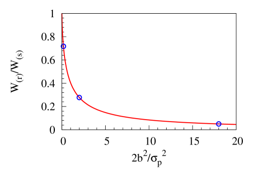
Figure 2: The dependence of loses on the relative amplitude ratio between the control beams $b$ calculated using equation (37). Three circles indicate three cases corresponding to $\sigma_{p}=10$ and $b=3$, $10$ and $30$.

The proposed shemes for transferring a vortex from the control laser beam to the regenerated probe beam avoid non-adiabaticit (absporption) losses at the center of the vortex due to application of an additional control laser. Yet there are another kind of losses in the energy of the regenerated probe beam, because a part of the stored probe beam remains frozen in the medium in the form of atomic spin excitations. Let us estimate those losses. Suppose that the incident pulse of the probe electric field $\mathcal{E}^{(\mathrm{s})}$ has a Gaussian intensity profile with a width $\sigma_{\mathrm{p}}$ along its transversal coordinate $\tilde{\rho}$ and a length $L_{\mathrm{vac}}$ in the propagation direction $z$. The total electric field energy entering the cloud of cold atoms is

$$W_{(\mathrm{s})}=2\pi\int_{0}^{+\infty}\tilde{\rho}\rmd\tilde{\rho}\int_{0}^{L_{\mathrm{vac}}}\rmd z\,|\mathcal{E}^{(\mathrm{s})}|^{2}=\frac{\pi}{2}L_{\mathrm{vac}}|\mathcal{E}_{0}|^{2}\sigma_{\mathrm{p}}^{2}\,.$$ (35)

The electric probe field at the retrieval stage is related to the stored on in a different way for two cases of the storage and retrieval considered above.

In the case of lambda storage and tripod retrieval, regenerated electric field is described by the equation (32). The length of the regenerated pulse is $L_{(\mathrm{r})}$. This length is related to the length $L_{\mathrm{vac}}$ of the initial pulse via the equation $L_{(\mathrm{r})}=L_{\mathrm{vac}}v_{\mathrm{g}}^{(\mathrm{s})}/v_{\mathrm{g}}^{(\mathrm{r})}$. Since the group velocity $v_{\mathrm{g}}^{(\mathrm{r})}$ in the retrieval stage depends transversal coordinate $\tilde{\rho}$, the length $L_{(\mathrm{r})}$ is also $\tilde{\rho}$ dependent. The total energy of electric field leaving the cloud is

$$W_{(\mathrm{r})} =2\pi\int_{0}^{+\infty}\tilde{\rho}\rmd\tilde{\rho}\int_{0}^{L_{(\mathrm{r})}}\rmd z\,|\mathcal{E}^{(\mathrm{r})}|^{2}$$ (36)

$$=\pi L_{\mathrm{vac}}|\mathcal{E}_{0}|^{2}\int_{0}^{+\infty}\frac{x\exp[-2x(\sigma_{\mathrm{r}}^{-2}+\sigma_{\mathrm{p}}^{-2})]}{x\exp(-2x/\sigma_{\mathrm{r}}^{2})+b^{2}\exp(-2x/\sigma_{\mathrm{r}3}^{2})}\rmd x\,.$$

Here $\sigma_{\mathrm{r}3}$ is the width of the second control beam at the retrieval stage $\Omega_{\mathrm{c}3}^{(\mathrm{r})}=bA\exp(-\tilde{\rho}^{2}/\sigma_{\mathrm{r}3}^{2})$. The energy losses may be found comparing the energies of the pulses before and after the interaction with the cloud. For simplicity suppose that $\sigma_{\mathrm{r}}=\sigma_{\mathrm{r}3}$. Then

$$\frac{W_{(\mathrm{r})}}{W_{(\mathrm{s})}} =\int_{0}^{+\infty}\frac{\rme^{-y}}{y+2b^{2}/\sigma_{\mathrm{p}}^{2}}y\rmd y$$ (37)

$$=1+\frac{2b^{2}}{\sigma_{\mathrm{p}}^{2}}\exp\left(\frac{2b^{2}}{\sigma_{\mathrm{p}}^{2}}\right)\mathop{\mathrm{Ei}}\left(-\frac{2b^{2}}{\sigma_{\mathrm{p}}^{2}}\right)\,.$$

If the intensity of the second control beam is large, $b\gg\sigma_{\mathrm{p}}$, the ratio of the energies is $W_{(\mathrm{r})}/W_{(\mathrm{s})}\approx\sigma_{\mathrm{p}}^{2}/(2b^{2})$.

In the case of tripod storiage and lambda retrieval the restored electric field profile is described by equation (34). Nevetheless the loses are found the same as in the previous case (37). Several values of $W_{(\mathrm{r})}/W_{(\mathrm{s})}$ are given in figure 2. When the amplitude ratio of the control beams $b$ increases, the loses are seen to increase.

4 Concluding remarks

We have considered propagation, storing and retrieval of slow light (probe beam) in a resonant atomic medium illuminated by two control laser beams of larger intensity. The probe and two control beams act on atoms in a tripod configuration of the light-matter coupling in which three hyperfine atomic ground states and one excited state are involved. The first control beam is allowed to have an orbital angular momentum (OAM). Application of the second vortex-free control laser ensures the adiabatic (lossles) propagation of the probe beam at the vortex core where the intensity of the first control laser goes to zero. Using the adiabatic approximation we have derived the equation of motion for the probe beam and analysed it in the case where one of the control beams has an optical vortex.

Storing and release of the probe beam is accomplished by switching off and on the control laser beams leading to the transfer of the optical vortex from the first control beam to the regenerated probe field. A part of the stored probe beam remains frozen in the atomic cloud in a form of spin excitations, a number of which increases with increasing the intensity of the second control laser. We have analysed such losses in the regenerated probe beam and provided conditions for the optical vortex of the control beam to be transferred efficiently to the restored probe beam.

We have investigated in detail two cases of storing and retrieval of optical vortices onto the atomic medium. In the first case the $\Lambda$ scheme is used for the storage, whereas the tripod setup is exploited for the retrieval. In such a situation the vortex can be transferred efficiently and without a distortion from the restoring control beam to the regenerated probe beam. In the second case the tripod system is used for the storing and the $\Lambda$ system is employed for the retrieval. The vortex is then transferred from the storing control beam to the regenerated probe in a phase conjugated form, so the regenerated probe beam acquires an opposite vorticity. The regenerated beam is then distorted and becomes narrower as compared to the storing beam. Thus it experiences a larger diffraction spreading in the subsequent propagation in the medium.

References

References

- [1] L. V. Hau, S. E. Harris, Z. Dutton, and C. H. Behroozi. Light speed reduction to 17 metres per second in an ultracold atomic gas. Nature, 397:594, 1999.
- [2] M. M. Kash, V. A. Sautenkov, A. S. Zibrov, L. Hollberg, G. R. Welch, M. D. Lukin, Y. Rostovtsev, E. S. Fry, and M. O. Scully. Ultraslow group velocity and enhanced nonlinear optical effects in a coherently driven hot atomic gas. Phys. Rev. Lett., 82:5229, 1999.
- [3] D. Budker, D. F. Kimball, S. M. Rochester, and V. V. Yashchuk. Nonlinear magneto-optics and reduced group velocity of light in atomic vapor with slow ground state relaxation. Phys. Rev. Lett., 83:1767, 1999.
- [4] I. Novikova, D. F. Phillips, and R. L. Walsworth. Slow light with integrated gain and large pulse delay. Phys. Rev. Lett., 99:173604, 2007.
- [5] O. Firstenberg, P. London, M. Shuker, A. Ron, and N. Davidson. Elimination, reversal and directional bias of optical diffraction. Nature Physics, 5:665, 2009.
- [6] M. Fleischhauer and M. D. Lukin. Dark-state polaritons in electromagnetically induced transparency. Phys. Rev. Lett., 84:5094, 2000.
- [7] C. Liu, Z. Dutton, C. H. Behroozi, and L. V. Hau. Observation of coherent optical information storage in an atomic medium using halted light pulses. Nature, 409:490, 2001.
- [8] D. F. Phillips, A. Fleischhauer, A. Mair, R. L. Walsworth, and M. D. Lukin. Storage of light in atomic vapor. Phys. Rev. Lett., 86:783, 2001.
- [9] G. Juzeliūnas and H. J. Carmichael. Systematic formulation of slow polaritons in atomic gases. Phys. Rev. A, 65:021601, 2002.
- [10] A. S. Zibrov, A. B. Matsko, O. Kocharovskaya, Y. V. Rostovtsev, G. R. Welch, and M. O. Scully. Transporting and time reversing light via atomic coherence. Phys. Rev. Lett., 88:103601, 2002.
- [11] M. F. Yanik and S. Fan. Stopping and storing light coherently. Phys. Rev. A, 71:013803, 2005.
- [12] G. Nikoghosyan. Storage and perpendicular retrieving of light pulses in electromagnetically induced transparency media. Eur. Phys. J. D, 36:119, 2005.
- [13] M. D. Eisaman, A. André, F. Massou, M. Fleischhauer, A. S. Zibrov, and M. D. Lukin. Electromagnetically induced transparency with tunable single-photon pulses. Nature, 438:837, 2005.
- [14] P.-C. Guan, Y.-F. Chen, and I. A. Yu. Role of degenerate zeeman states in the storage and retrieval of light pulses. Phys. Rev. A, 75:013812, 2007.
- [15] N. S. Ginsberg, S. R. Garner, and L. V. Hau. Coherent control of optical information with matter wave dynamics. Nature, 445:623, 2007.
- [16] U. Schnorrberger, J. D. Thompson, S. Trotzky, R. Pugatch, N. Davidson, S. Kuhr, and I. Bloch. Electromagnetically induced transparency and light storage in an atomic mott insulator. Phys. Rev. Lett., 103:033003, 2009.
- [17] R. Zhang, S. R. Garner, and L. V. Hau. Creation of long-term coherent optical memory via controlled nonlinear interactions in bose-einstein condensates. Phys. Rev. Lett., 103:233602, 2009.
- [18] F. Beil, M. Buschbeck, G. Heinze, and T. Halfmann. Light storage in a doped solid enhanced by feedback-controlled pulse shaping. Phys. Rev. A, 81:053801, 2010.
- [19] M. Bajcsy, A. S. Zibrov, and M. D. Lukin. Stationary pulses of light in an atomic medium. Nature, 426:638, 2003.
- [20] S. A. Moiseev and B. S. Ham. Quantum manipulation of two-color stationary light: Quantum wavelength conversion. Phys. Rev. A, 73:033812, 2006.
- [21] M. Fleischhauer, J. Otterbach, and R. G. Unanyan. Bose-einstein condensation of stationary-light polaritons. Phys. Rev. Lett., 101:163601, 2008.
- [22] F. E. Zimmer, J. Otterbach, R. G. Unanyan, B. W. Shore, and M. Fleischhauer. Dark-state polaritons for multicomponent and stationary light fields. Phys. Rev. A, 77:063823, 2008.
- [23] Y.-W. Lin, W.-T. Liao, T. Peters, H.-C. Chou, J.-S. Wang, H.-W. Cho, P.-C. Kuan, and I. A. Yu. Stationary light pulses in cold atomic media and without bragg gratings. Phys. Rev. Lett., 102:213601, 2009.
- [24] J. Otterbach, J. Ruseckas, R. G. Unanyan, G. Juzeliūnas, and M. Fleischhauer. Effective magnetic fields for stationary light. Phys. Rev. Lett., 104:033903, 2010.
- [25] R. G. Unanyan, J. Otterbach, M. Fleischhauer, J. Ruseckas, V. Kudriašov, and G. Juzeliūnas. Spinor slow-light and dirac particles with variable mass. Phys. Rev. Lett., 105:173603, 2010.
- [26] E. Arimondo. Progress in Optics. Elsevier, Amsterdam, 1996.
- [27] S. E. Harris. Electromagnetically induced transparency. Physics Today, 50:36, 1997.
- [28] M. O. Scully and M. S. Zubairy. Quantum Optics. Cambridge University Press, Cambridge, 1997.
- [29] M. D. Lukin. Colloquium: Trapping and manipulating photon states in atomic ensembles. Rev. Mod. Phys., 75:457, 2003.
- [30] M. Fleischhauer, A. Imamoglu, and J. P. Marangos. Electromagnetically induced transparency: Optics in coherent media. Rev. Mod. Phys., 77:633, 2005.
- [31] J. Appel, E. Figueroa, D. Korystov, M. Lobino, and A. I. Lvovsky. Quantum memory for squeezed light. Phys. Rev. Lett., 100:093602, 2008.
- [32] K. Honda, D. Akamatsu, M. Arikawa, Y. Yokoi, K. Akiba, S. Nagatsuka, T. Tanimura, A. Furusawa, and M. Kozuma. Storage and retrieval of a squeezed vacuum. Phys. Rev. Lett., 100:093601, 2008.
- [33] K. Akiba, K. Kashiwagi, M. Arikawa, and M. Kozuma. Storage and retrieval of nonclassical photon pairs and conditional single photons generated by the parametric down-conversion process. New J. Phys., 11:013049, 2009.
- [34] U. Leonhardt and P. Piwnicki. Relativistic effects of light in moving media with extremely low group velocity. Phys. Rev. Lett., 84:822, 2000.
- [35] P. Öhberg. Slow light and the phase of a bose-einstein condensate. Phys. Rev. A, 66:021603, 2002.
- [36] M. Fleischhauer and S. Gong. Stationary source of nonclassical or entangled atoms. Phys. Rev. Lett., 88:070404, 2002.
- [37] G. Juzeliūnas, M. Mašalas, and M. Fleischhauer. Storing and releasing light in a gas of moving atoms. Phys. Rev. A, 67:023809, 2003.
- [38] M. Artoni and I. Carusotto. In situ velocity imaging of ultracold atoms using slow light. Phys. Rev. A, 67:011602, 2003.
- [39] F. Zimmer and M. Fleischhauer. Sagnac interferometry based on ultraslow polaritons in cold atomic vapors. Phys. Rev. Lett., 92:253201, 2004.
- [40] M. Padgett, G. Whyte, J. Girkin, A. Wright, L. Allen, P. Öhberg, and S. M. Barnett. Polarization and image rotation induced by a rotating dielectric rod: an optical angular momentum interpretation. Optics Letters, 31:2205, 2006.
- [41] J. Ruseckas, G. Juzeliūnas, P. Öhberg, and S. M. Barnett. Polarization rotation of slow light with orbital angular momentum in ultracold atomic gases. Phys. Rev. A, 76:053822, 2007.
- [42] L. Allen, M. J. Padgett, and M. Babiker. The orbital angular momentum of light. Prog. Opt., 39:291, 1999.
- [43] L. Allen, S. M. Barnett, and M. J. Padgett. Optical Angular Momentum. Institute of Physics Publishing, Bristol, 2003.
- [44] Z. Dutton and J. Ruostekoski. Transfer and storage of vortex states in light and matter waves. Phys. Rev. Lett., 93:193602, 2004.
- [45] R. Pugatch, M. Shuker, O. Firstenberg, A. Ron, and N. Davidson. Topological stability of stored optical vortices. Phys. Rev. Lett., 98:203601, 2007.
- [46] T. Wang, L. Zhao, L. Jiang, and S. F. Yelin. Diffusion-induced decoherence of stored optical vortices. Phys. Rev. A, 77:043815, 2008.
- [47] D. Moretti, D. Felinto, and J. W. R. Tabosa. Collapses and revivals of stored orbital angular momentum of light in a cold-atom ensemble. Phys. Rev. A, 79:023825, 2009.
- [48] R. Unanyan, M. Fleischhauer, B. W. Shore, and K. Bergmann. Robust creation and phase- sensitive probing of superposition states via stimulated raman adiabatic passage (stirap) with degenerate dark states. Opt. Commun., 155:144, 1998.
- [49] E. Paspalakis and P. L. Knight. Electromagnetically induced transparency and controlled group velocity in a multilevel system. Phys. Rev. A, 66:015802, 2002.
- [50] S. Rebic, D. Vitali, C. Ottaviani, P. Tombesi, M. Artoni, F. Cataliotti, and R. Corbalán. Polarization phase gate with a tripod atomic system. Phys. Rev. A, 70:032317, 2004.
- [51] D. Petrosyan and Y. P. Malakyan. Magneto-optical rotation and cross-phase modulation via coherently driven four-level atomsin a tripod configuration. Phys. Rev. A, 70:023822, 2004.
- [52] T. Wang, M. Kostrun, and S. F. Yelin. Multiple beam splitter for single photons. Phys. Rev. A, 70:053822, 2004.
- [53] J. Ruseckas, G. Juzeliūnas, P. Öhberg, and M. Fleischhauer. Non-abelian gauge potentials for ultracold atoms with degenerate dark states. Phys. Rev. Lett., 95:010404, 2005.
- [54] I. E. Mazets. Adiabatic pulse propagation in coherent atomic media with the tripod level configuration. Phys. Rev. A, 71:023806, 2005.
- [55] A. Raczynski, M. Rzepecka, J. Zaremba, and S. Zielinska-Kaniasty. Polariton picture of light propagation and storing in a tripod system. Opt. Commun., 260:73, 2006.
- [56] A. Raczynski, J. Zaremba, and S. Zielinska-Kaniasty. Beam splitting and hong-ou-mandel interference for stored light. Phys. Rev. A, 75:013810, 2007.
- [57] A. Raczynski, K. Slowik, J. Zaremba, and S. Zielinska-Kaniasty. Controlling statistical properties of stored light. Opt. Commun. 279 (2007) 324–329, 279:324, 2007.
- [58] N. Gavra, M. Rosenbluh, T. Zigdon, A. D. Wilson-Gordon, and H. Friedmann. Sub-doppler and sub-natural narrowing of an absorption line. Opt. Comm., 280:374, 2007.
- [59] J. Ruseckas, A. Mekys, and G. Juzeliūnas. Manipulation of slow light with orbital angular momentum in cold atomic gases. Optics and Spectroscopy, 108:438, 2010.
- [60] G. Juzeliūnas, P. Öhberg, J. Ruseckas, and A. Klein. Effective magnetic fields in degenerate atomic gases induced by light beams with orbital angular momenta. Phys. Rev. A, 71:053614, 2005.