Active Longitudes Revealed by Large-scale and Long-lived Coronal Streamers

Abstract

We use time-series ultraviolet full sun images to construct limb-synoptic maps of the Sun. On these maps, large-scale, long-lived coronal streamers appear as repetitive sinusoid-like arcs projected over the polar regions. They are caused by high altitude plasma produced from sunspot-rich regions at latitudes generally far from the poles. The non-uniform longitudinal distribution of these reveals four longitudinal zones at the surface of the sun from which sunspots erupt preferentially over the 5-year observing interval (2006 January to 2011 April). Spots in these zones (or “clusters”) have individual lifetimes short compared to the lifetimes of the coronal features which they sustain, and erupt at different times. The four sunspot clusters contain $>75$% of all numbered sunspots in this period. They occupy two distinct longitudinal zones separated by $\sim 180^{\circ}$ and each spanning $\sim 100^{\circ}$ in longitude. The rotation rates of the spot clusters are $\sim$5% faster than the rates at both the surface and the bottom of the convection zone. While no convincing theoretical framework exists to interpret the sunspot clusters in the longitude-time space, their persistent and nonuniform distribution indicates long-lived, azimuthal structures beneath the surface, and are compatible with the existence of previously-reported active longitudes on the sun.

1 Introduction

While it may appear locally chaotic, the Sun’s activity is well known to be globally ordered and shows a number of distinct patterns. Summarized by Babcock (1961), observations of sunspots reveal Hale’s law of hemispheric polarity (Hale et al., 1919), Joy’s law of polarity pair orientation, and Spörer’s law of zone as well as Maunder’s sunspot butterfly diagram through the 11-year solar activity cycle, and 22-year magnetic cycle. These well established observations converge with recent discoveries on surface flows, notably the torsional oscillation and the meridional flow (Howard & Labonte, 1980; Devore et al., 1984; Hathaway, 1996; Wang et al., 2002; Vorontsov et al., 2002; Hathaway & Rightmire, 2010). These observations laid foundations for modeling solar global magnetic fields from the Babcock-Leighton’s schematic dynamo model (Babcock, 1961; Leighton, 1969) to recent more advanced models (Wang et al., 1991; Dikpati & Charbonneau, 1999; Charbonneau, 2010). An ultimate goal is to understand the rise and fall of the global magnetic field and so to predict solar cycles.

On other stars, the existence of long-lived active longitudes (regions prone to produce an excess number of spots) is well established (Berdyugina & Tuominen, 1998). Active longitudes have been reported on the Sun for many decades, but their existence is not without controversy and they do not find an explanation in standard models of the solar dynamo. The tendency of new sunspot groups to emerge in the neighborhood of previously existing sunspots for several consecutive solar rotations was observed, especially during the solar activity minimum (Gaizauskas et al., 1994, 1998; van Driel-Gesztelyi et al., 2003). So-called “complexes of activity” on the sun were reported from a statistical study of the sunspot distribution over 128 years and from synoptic maps of photospheric magnetic fields (Bogart, 1982; Gaizauskas et al., 1983; Berdyugina & Usoskin, 2003; Olemskoy & Kitchatinov, 2009). Solar flares, which occur mostly in association with active regions, are found to concentrate on “active zones” similar to the behavior of sunspots (Bai, 1987). The analyses of high-flare-activity sunspot regions led to the existence of two “giant longitude zones” with one of them flare-richer than the other (Shelke & Shelke, 1989; Rodriguez Taboada & Gil Moreno, 1993). Analysis of GOES X-ray solar flare data lead to a similar conclusion, with two active longitudinal zones separated by $180^{\circ}$ (Zhang et al. (2011)). “Sunspot nests” or “sunspot clusters” were also found by a single-linkage clustering technique used to trace the photospheric sunspots in longitude, latitude and time (Brouwer & Zwaan, 1990).

In this work, we use long-lived coronal streamers linked to underlying active regions as a proxy by which to study the longitudinal distribution of sunspot groups on the Sun. Benefiting from a large amount of uninterrupted coronal emission data on the entire sun from space, we demonstrate that the large-scale, long-lived coronal streamers directly reflect “sunspot active longitudes” in the photosphere. In an earlier study, close inspection and a schematic model showed that these streamers are connected with more equatorial active regions (Li et al., 2000). During the period April 1996 to May 1997 ($\sim 1$ year), three distinct coronal streamers with life spans as long as 10 solar rotations were found to be sustained by three distinct regions from where sunspots emerged. The sunspot groups erupt from a localized region of the sun, but at different times (Li et al., 2002). The current study has more than 5 year (January 2006-April 2011) time coverage (compared with 1 year in the previous study) and during this period, the solar activity passed from the declining phase to the minimum and to the ascending phase. The new observations point to the little-studied, non-axisymmetric nature of the global solar magnetic field (Stix, 1971; D’Silva & Choudhuri, 1993; Dikpati & Gilman, 2005; Berdyugina et al., 2006).

2 Data

Two sets of data are employed in this study: full sun coronal EUV images and photospheric sunspot records.

The full sun images are obtained by EUV imagers from space, which record the FeXII 195 Å line, for which the effective plasma temperature is $\sim$1.5 MK. As a result, coronal emissions are more prominent in the active regions than in coronal holes and the quiet Sun, where the temperature is normally below 1.5 MK (Aschwanden et al., 2007). For the period between 2006 January 1 and 2006 December 3, we use images taken by the Extreme ultraviolet Imaging Telescope (EIT) (Delaboudinière et al., 1995) onboard SoHO (Domingo et al., 1995). For the period after 2006 December 4, we use images taken by the Extreme UltraViolet Imager (EUVI) (Howard et al., 2008), a part of the Sun Earth Connection Coronal and Heliospheric Investigation (SECCHI) package on board STEREO (Kaiser et al., 2008).

The STEREO spacecraft are separated from the Earth by a large and time-dependent difference in ecliptic longitude. To compare sunspot records obtained from the Earth with the EUVI/STEREO images, this longitude difference has to be taken into account. For this, we use the World Coordinate System recorded in the STEREO FITS headers (Thompson, 2006; Thompson & Wei, 2010). The spacecraft heliographic longitudes are subtracted from the sunspot disk longitudes as if the sunspots are viewed from STEREO A. For example, the sunspot group NOAA 11045 was reported at W17N23 on 2010 February 9 as viewed from the Earth, but its disk location was E47N23 after correction to the location of STEREO A. The sunspot disk locations are corrected in this way when the coronal images taken with STEREO A and B are used, but no correction was made when SoHO/EIT data are used, since SoHO’s longitude remains close to that of the Earth.

The photospheric sunspot daily records known as the Solar Region Summary (SRS) are compiled by the Space Weather Prediction Center (SWPC, http://www.swpc.noaa.gov/) from approximately a dozen observatories reporting observations in real time. In the SRS records, each sunspot group is assigned a number, known as the NOAA number, during its disk passage. Also included are observing dates, disk locations, Carrington longitudes and latitudes of the sunspots, the longitudinal extents of groups in heliographic degrees, the total corrected sunspot group area in millionths of the solar hemisphere (equal to 3$\times$10⁶ km²), the total number of sunspots visible in the group, and a magnetic classification of the group.

For convenience, the time is measured as Day of Year (DOY), where we define DOY=1 as 2006 January 1.

3 Large-scale, Long-lived Coronal Streamers

Our findings are based on the study of the large-scale, and long-lived coronal streamers in the EUV coronal emission data. These streamers are found to be largely associated with more equatorial active regions, but are often seen at high latitudes due to projection effect (Li et al., 2000).

3.1 Large-scale Coronal Streamers

On individual images, large coronal streamers extending from active regions are best observed at soft X-ray wavelengths (c.f. Figure 2 of Li et al. (2002) or the movie at URL http://www2.ess.ucla.edu/ jingli/movie_sxt/AlMg_19960727-19960921.html). This is because these streamers have temperatures $\sim 2.0$ MK (e.g. Li et al. (1998)), which are well-matched to the effective temperature range sampled by the imagers on Yohkoh/SXT (Tsuneta et al., 1991).

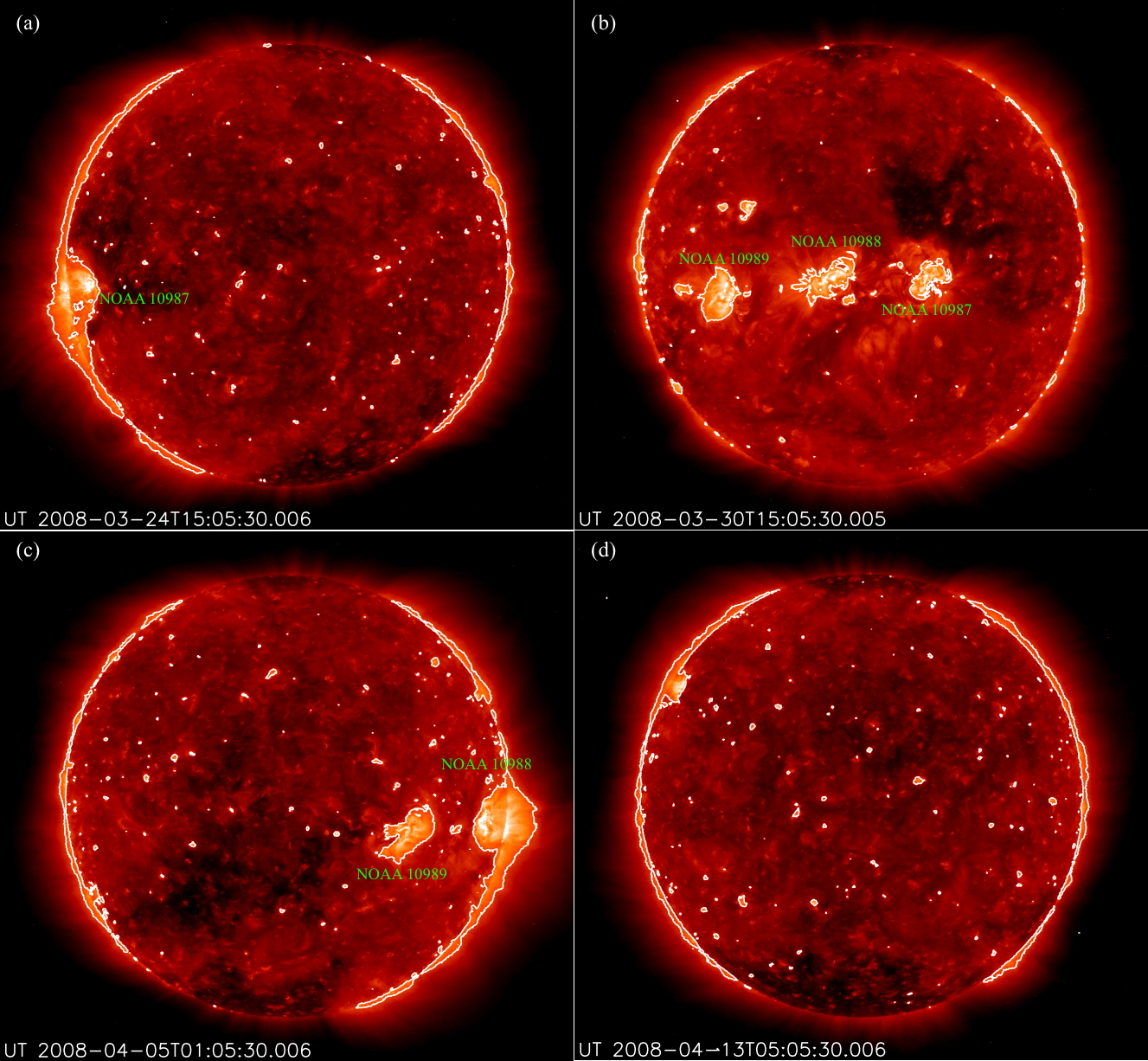
Figure 1: The coronal emission images taken with EUVI/STEREO A in 195 Å. Contours represent brightness levels at 4.5, 45.0 and 450.0 times the median disk emission. Bright patches correspond to the active regions. Active regions appear (a) on the east limb, (b) disk center, (c) the west limb and (d) the far side of the sun.

With EUV images, Fig. 1 illustrates how the limb brightness varies as active regions are carried round by the solar rotation. In general, coronal emission lines are optically thin. The integral along the line of sight leads to stronger emissions on east and west limbs than those on limbs near polar holes (see all panels in Fig. 1). This is simply because equatorial regions are sources of strong coronal EUV emissions due to concentrations of active regions. When sunspot groups are near the solar limb, bright emissions are enhanced from the equator to polar regions. In panels (a) and (c), streamers outlined by contours extend from active regions to high latitudes. However, they do not cover the polar holes, indicating that these high latitude streamers are longitudinally aligned with active regions. They extend largely to high latitude through either the projection effect or by having magnetic anchors at high latitudes. When active regions are on the disk, the limb emissions are no longer intense, but, for example, the southern polar hole becomes invisible (see Panel (b)). This is because the high latitude streamers associated with the active regions appears as a large hot blob at high altitude covering the polar hole when projected onto the plane of the sky. Active regions carried to the far side of the sun produce weak limb emissions, but the southern polar hole is visible (Panel (d)). This is because the high latitude streamers connected with active regions are on the far side of the sun. They are projected to the plane of the sky, but are behind the solar disk. Variations in the shapes of polar holes corresponding to the projected locations of active regions on either east or west limbs were also reported by Sheeley et al. (1989) using coronal images at He I 10830 Å. Comparing HeI 10830 images with the photospheric magnetograms, they interpreted the observations as the result of the reconnections between the polar magnetic field and the newly erupted large bipolar regions.

3.2 Long-Lived Coronal Streamers

Variations in the appearance/disappearance of the polar coronal holes and in the more equatorial limb brightness are best displayed on a so-called coronal Limb Synoptic Map (LSM) (Li et al., 2000). The practical advantage conveyed by LSMs over conventional Carrington maps is that variations in limb activity occurring on timescales that are very long compared to a solar rotation can be easily seen. Fig. 2 shows a sample LSM centered on the South Pole for the period Jan 30 to Apr 29, 2008. A long-lived streamer appears as a diagonal streak crossing over the southern polar hole on three consecutive solar rotations. This pole-crossing feature is the same dense, hot plasma seen on individual images extending from active regions to heights large enough that it is visible above the limb near the pole.

If the solar spin axis were perpendicular to the ecliptic plane, polar streamers caused by projection would appear as nearly perfect sinusoidal patterns against the polar holes on LSM. In reality, the solar spin axis is inclined to the ecliptic normal by an angle 7.25${\arcdeg}$, so that the projected tilt along the line of sight varies between $-7.25^{\circ}$ to $7.25^{\circ}$ through the year. This seasonal variation in the projected tilt is responsible for an observed asymmetry in the polar streamers, such that the rising and falling sides of a polar sinusoid are not in general equally bright (Li et al., 2000). For example, in Fig. 2, the branches from the west to east limbs (the “falling branches”, formed when responsible active regions are on the far side of the sun) are more prominent than those from the east to west limbs (“rising branches”, formed when responsible active regions are on visible side of the sun). This asymmetry is introduced by the non-zero heliographic latitude of the Sun ($B_{0}$ fell in the range $-7.3^{\circ}$ to $-1.3^{\circ}$ viewed from STEREO A in the interval plotted in Figure 2). The closer is $B_{0}$ to zero, the more symmetric are the rising and falling branches of the long-lived streamer and the sense of the asymmetry reverses as $B_{0}$ changes sign.

To give a sense of the life spans of long-lived coronal streamers, Fig. 3 shows the LSM made from EUV images taken between the end of 2006 and the end of 2010. We have plotted the total range of polar angles from $90^{\circ}$ to $450^{\circ}$ so that both polar holes (at 180$\arcdeg$ and 360$\arcdeg$) are displayed uninterrupted by the axes of the figure. The long-lived coronal streamers are seen as repetitive, inclined structures crossing the dark polar holes (marked NP for North Pole and SP for South Pole), in both hemispheres in Figure 3. Other prominent features of the LSMs are periodic bright patches near the equator on the east ($\sim 90^{\circ}$) and west ($\sim 270^{\circ}$) limbs. They are active regions carried to the east to the west limbs by solar rotation and showing evolution in size and brightness from rotation to rotation. That they always appear as extensions of long-lived streamers indicates a physical connection between the streamers and the active regions.

The long-lived streamers have lifetimes longer than typical sunspots because they are replenished by the continuous emergence of active regions in the photosphere. The idea was also proposed by Sheeley & Devore (1986) who explained the recurrent patterns of solar magnetic field with periods 28- to 29-day. In their view, “the patterns are caused by longitudinal fluctuations in the eruption of new magnetic flux, the transport of this flux to mid latitudes by supergranular diffusion and meridional flow”. The long-lived coronal streamers necessarily large-scale because they must extend high enough to be seen in projection above the polar regions in order to be detected on LSMs. It is the structured distribution of these long-lived streamers in Fig 3 which provides the basic evidence for long-lived, non-randomly distributed coronal structures on the sun and for the underlying active longitudes of sunspots. In the present data we find numerous long-lived streamers with lifetimes $>$5 solar rotations. The longest lasting coronal streamer was observed in the last solar minimum between 1996 April 9 and 1997 February 3, corresponding to more than 10 solar rotations (Li et al., 2002).

4 Sunspot Active Longitudes

The active longitudes are the longitudinal bands from where the sunspots erupted repeatedly over a long period of time. The term is equivalent to sunspots clustering in longitude-time space, or non-contemporaneous spot cluster. The method to detect the spot cluster can be summarized in two basic steps: (1) large-scale, long-lived coronal streamers on the coronal LSM are connected with sunspot groups; (2) more members of a spot cluster are identified based on having Carrington longitudes in the vicinity of those spot groups already belonging to a spot cluster.

4.1 Sunspot Clusters by Long-lived Coronal Streamers

The long-lived coronal streamer on the LSM can be modeled by considering the apparent sky-plane motion of a radial coronal structure as it is carried round by the solar rotation. This is equivalent to the scenario that coronal streamers are rooted at the active regions, and extend radially to high altitudes. The projected latitude, $\theta$, of such a structure as a function of time is given by:

$$\theta(t)=\arctan\left(\cos B_{0}\frac{\tan B}{\cos L(t)}-\tan L(t)\sin B_{0}\right),$$ (1)

where $B_{0}$ is the heliographic latitude of the solar center and $B$ is the Carrington latitude where the coronal structure is rooted. Quantity $L(t)$ is the solar disk longitudinal position of the sunspot group as a function of time, given by

$$L(t)=\Omega(t-t_{0}),$$

where $t_{0}$ is the time when the sunspot group crosses the east limb and $\Omega=\omega(B)-\omega_{obs}$ is the solar synodic rotation rate in which $\omega(B)$ is the sidereal rotation rate appropriate to latitude $B$. The function $\omega(B)$ is the subject of many past and continuing studies (Beck, 2000; Li et al., 2011). We used the differential rotation of Newton & Nunn (1951), in which $\omega(B)=a+b\sin^{2}B$, where $a=14^{\circ}.38$ day^-1 and $b=-2.^{\circ}96$ day^-1. We adopted $\omega_{obs}=360/346$ ^∘day^-1 for STEREO A ($360/388$ ^∘day^-1 for STEREO B) to account for the drift motions of these spacecraft. With Equations (1) and (4.1), a radial plasma structure above an active region describes a sinusoidal curve on a LSM. This is shown in the figure 2 in which a long-lived streamer is traced by a number of sinusoidal curves (dotted curves). The long-lived streamer varies in phase with the NOAA-numbered sunspots, which jump from the east to the west limbs as they are carried round by solar rotation. Dotted sinusoidal curves have the same phases and periods as sunspot groups marked with NOAA numbers, but are rooted at latitude $B=-65^{\circ}$. This indicates that the active regions and the high latitude streamers are longitudinally locked and rigidly connected. These sunspot groups are members of a sunspot cluster because their corresponding polar sinusoidal curves collectively fit to a long-lived coronal streamer.

Sunspots corresponding to a long-lived coronal streamer in Fig. 2 have the following properties: (1) they appear on either the east or the west limb; (2) they give rise to large-scale streamers projecting to high latitudes; (3) their corresponding polar sinusoidal curves calculated with Equations (1) and (4.1) on a LSM unambiguously match a long-lived streamer. About 50% of sunspots in a cluster are identified in this step.

4.2 Spot Cluster Membership based on Longitudinal Preference

If the sun rotated rigidly at the Carrington rotation rate, $\omega_{cr}$, we would see sunspot groups emerging in the vicinity of a fixed Carrington longitude one rotation after another. The long-lived streamers on a LSM would have the same period as the Carrington rotation period. In reality, the Carrington longitude of an active region drifts in time due to differential rotation:

$$\lambda(t)=\lambda_{0}(t_{0})+[\omega-\omega_{cr}](t-t_{0})$$ (2)

where $\lambda_{0}$ is the emerging sunspot Carrington longitude at $t_{0}$; $\omega$ is the rotation rate of the sunspot; $\omega_{cr}=14.18^{\circ}$ day^-1 is the sidereal Carrington rotation rate.

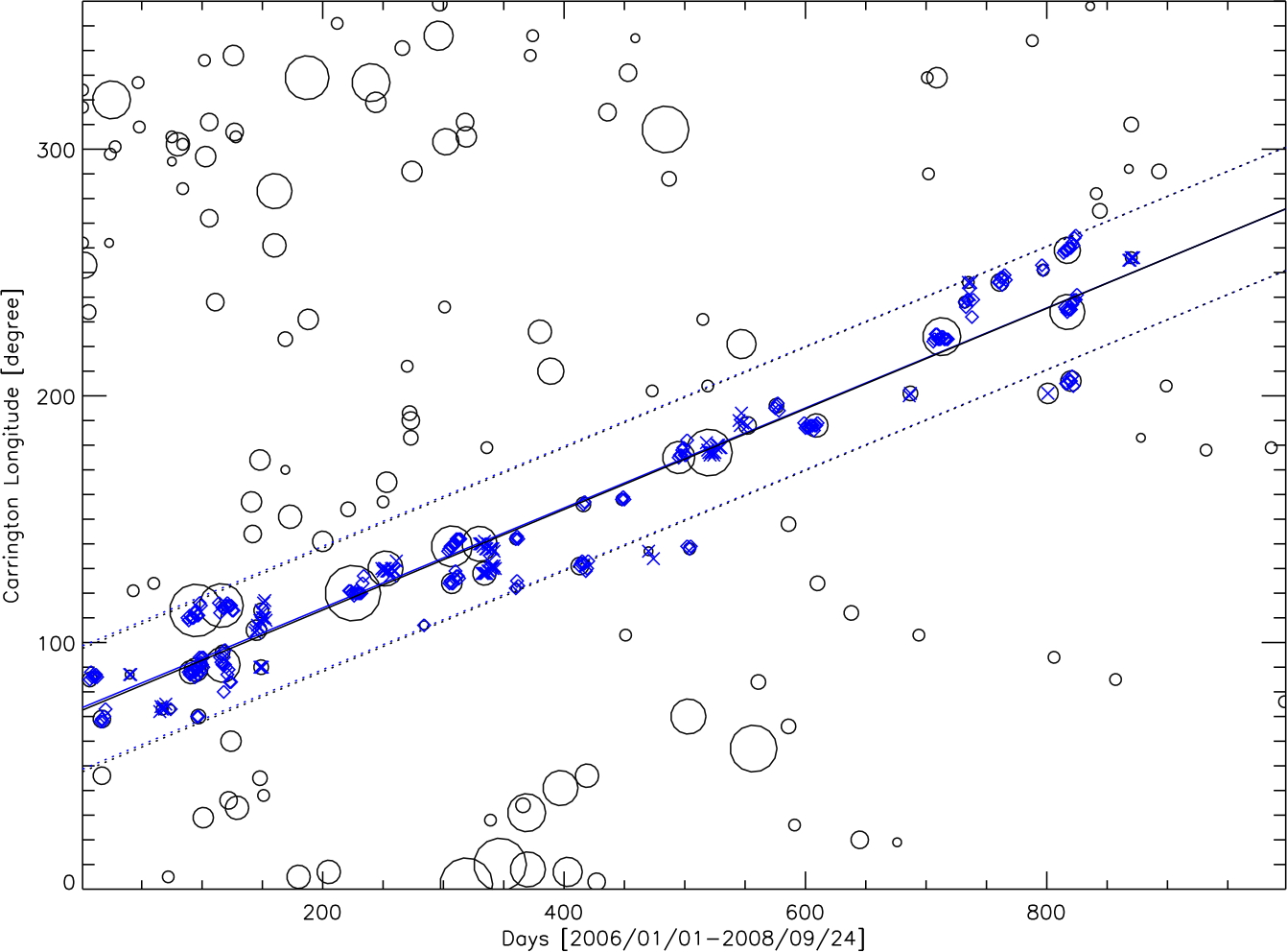
Figure 4: Carrington longitudes of sunspot groups as functions of time. All sunspot groups emerging between 2006 January 1 (DOY 1) and 2008 September 24 (DOY 998) are plotted with circles whose radii are proportional to the sunspot radii , $\sqrt{s}/\pi$, where “$s$” is the sunspot group area recorded in SRS. The sunspots in blue colors are members of a non-contemporaneous cluster. The sunspots with blue “$\diamond$” are identified by a long-lived polar sinusoidal streamer. A linear regression fit of these sunspots is plotted in a blue straight line. The longitudinal range of $\pm 25^{\circ}$ about the line is defined by blue dotted lines. The blue “$\times$” represent added sunspots to the existing spot cluster because they distribute within the two dotted blue lines. A black solid straight line is the linear regression fit to all members of the spot cluster. Note that there is only a little difference between the black and blue lines.

Fig.4 is an example of how sunspot groups are added to an existing non-contemporaneous sunspot cluster. All sunspot groups emerging between 2006 January 1 and 2008 September 24 (DOY 998) are plotted with circles on the Carrington longitude versus time plot. The radii of the circles are proportional to the sunspot group radii, $\sqrt{s}/\pi$, where “$s$” is the sunspot group area obtained from the SRS. The sunspot groups colored with blue “$\diamond$” are those identified with a long-lived streamer in step 1. Essentially all large spots in the cluster are identified in this way. Small spots evidently do not produce plasma structures tall enough to be seen in projection over the poles, and therefore do not form polar streamers. A linear regression fit of blue $\diamond$ spots with $\pm 25^{\circ}$ border lines define the range of Carrington longitudes of a spot cluster. Sunspot groups falling inside this longitudinal range, but are not previously recognized as the members of the cluster in step 1, are marked with blue “x”. These are new members to the existing spot cluster. About 50% of the spots in a cluster are identified in this way. The black solid line is a linear regression fit to all members of the spot cluster. The properties of the spot clusters do not depend on whether we use only those sunspots identified using the polar streamers as proxies or the totality of sunspots identified in steps (1) and (2), above.

5 Results and Discussions

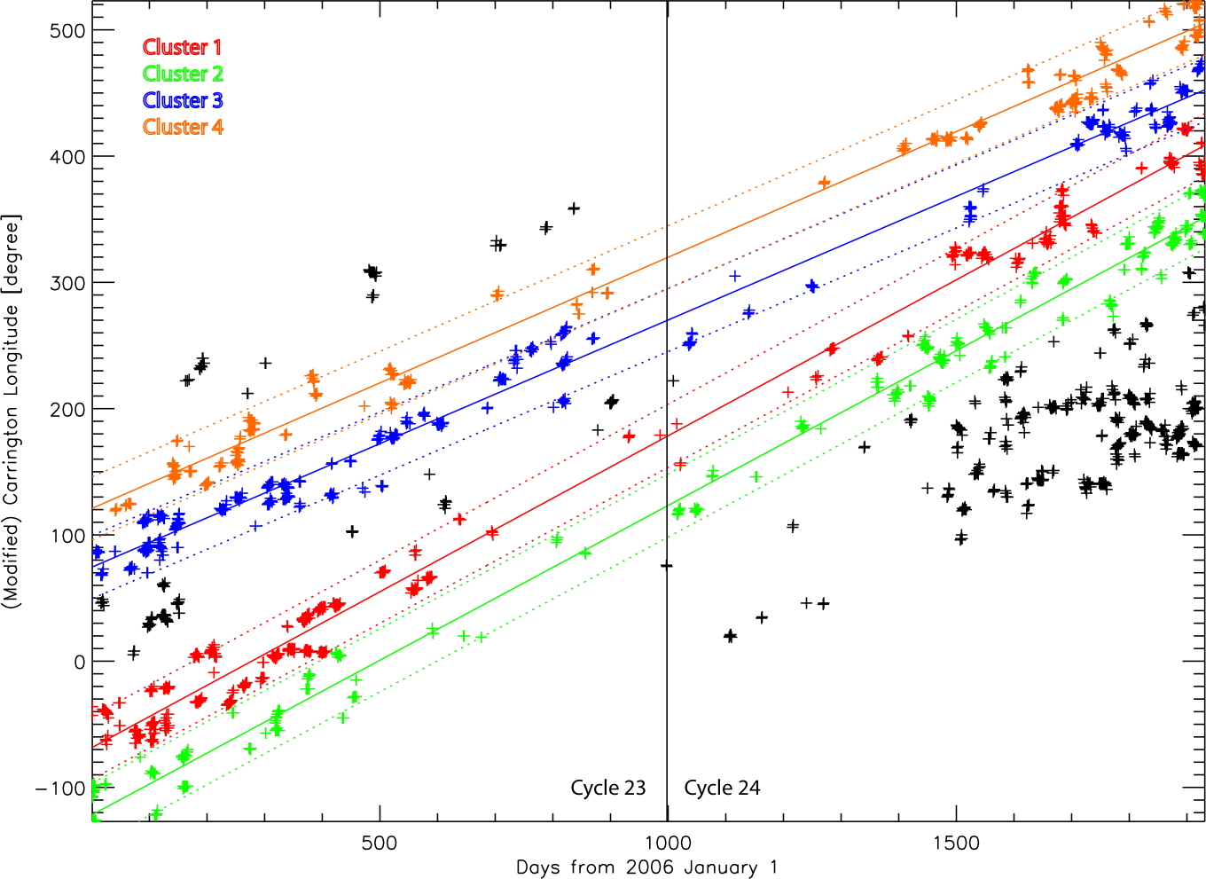
Figure 5: Carrington longitudes of sunspots as function of time between 2006 January 1 and 2011 April 11. Members of non-contemporaneous clusters are plotted in colored “+”. The linear regression fits of Carrington longitudes and $\pm 25^{\circ}$ of the fits are drawn with colored straight and dotted lines. Color schemes are used to represent sunspot groups associated with respective non-contemporaneous sunspot clusters: red, green, blue and orange represent spot clusters 1, 2, 3 and 4, respectively. The Carrington longitudes of some sunspots have been added or subtracted by $360^{\circ}$ to avoid artificial roll over from $360^{\circ}$ to $0^{\circ}$ within a cluster. The vertical straight line is drawn at DOY=998 (2008 September 24) separates the cycle 23 from 24. The sunspot groups found having no clear affiliation with any clusters at the present time are marked with black “+”.

Figure 5 plots all sunspot groups recorded between 2006 January 1 and 2011 April 15. More than 75% of numbered sunspots during this period are members of four spot clusters, which are plotted in the figure with differently colored symbols. Additional spot groups having no affiliation with any cluster are marked with black “+”. (We note that, although those spots cannot be associated with a cluster based on any repetitive coronal structures, their collective longitudinal distribution does appear non-random in Fig.5). In the current discussion, we will focus on the four sunspot clusters. In the Figure, we have added or subtracted $360^{\circ}$ to/from the Carrington longitudes of some sunspots of clusters in order to avoid artificial roll-over as a spot longitude drifts upwards from below $360^{\circ}$. DOY 998 (2008 September 24) is designated the end of cycle 23 based on the time when major sunspots first appeared at high latitudes (see the vertical line). All four spot clusters contain sunspot members emerging in both cycles 23 and 24. In other words, the clusters persist across the boundary between solar activity cycles.

From Fig. 5, a number of properties of a spot cluster are drawn and they are summarized in Table 1. In the Table, the median Carrington latitude, $\bar{B}$, is the median of the latitudes of all the sunspots within a cluster. From the linear regression fits of sunspot Carrington longitudes against time within a spot cluster (see straight lines going through each cluster in Fig.5), we obtain $\lambda_{0}$, the Carrington longitude at time $t_{0}=0$. The slope of the linear regression fits (c.f. Equation 2) gives, $k=\omega-\omega_{cr}$ ($\omega_{cr}$ is the Carrington rotation rate), and each spot cluster corresponds to a constant $\omega$. The surface sidereal rotation rates, $\omega(\bar{B})$, are calculated from the differential rotation of Howard & Harvey (1970), which measures the surface rotation rates using the spectral line shift data recorded at Mt. Wilson. Finally, synodic rotation periods for Earth are given in the last column, derived from the cluster common rotation rates, $\omega$.

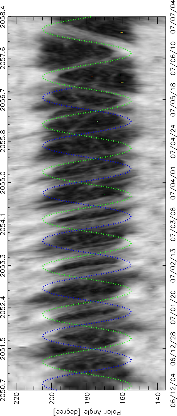
Figure 6: Two long-lived coronal streamers are traced by sinusoidal curves against southern polar hole ($180^{\circ}$) between 2006 December 4 and 2007 August 23 (the vertical axis varies from $135^{\circ}$ to $225^{\circ}$). They correspond to clusters 2 and 3. The green and blue dotted curves are calculated with the equations (1) and(4.1). They are rooted at $B=-65^{\circ}$ and have periods 26.88 and 26.99 [days] ($=360^{\circ}/(\omega-\omega_{obs})$. $\omega$ is the cluster rotation rate, and $\omega_{obs}=360^{\circ}/346$ for STEREO A), respectively.

What Fig. 5 has revealed is that a spot cluster corresponds to a single rotation rate, $\omega$. The rotation rate also describes the period of a long-lived coronal streamer on a LSM. This is shown in Fig. 6 in which the dotted curves calculated with equations (1) and (4.1) trace two long-lived coronal streamers. They correspond to spot clusters 2 and 3 having $\omega=14.43^{\circ}$ day^-1 and $14.38^{\circ}$ day^-1, respectively, but are rooted at $-65^{\circ}$ latitude. As we have discussed before, these long-lived streamers are connected with more equatorial active regions. Although two long-lived streamers have slight different rotation periods, 26.88 and 26.99 days, respectively, this may not be detected when they are used as tracers to measure the coronal rotation. The fact that each sinusoidal curve follows a single period indicates that corona likely appears to rotate constantly and rigidly when large-scale streamers are used as tracers. This is consistent with past observations using the long-lived streamers (Antonucci & Svalgaard, 1974a; Fisher & Sime, 1984; Sime et al., 1989). They concluded that the corona rotates more rigidly and faster than the photosphere. On the other hand, the short-lived coronal activity tends to show the same differential rotation as in the photosphere (Antonucci & Svalgaard, 1974a; Insley et al., 1995; Hara, 2009). The close relationship between the coronal rotation and photospheric magnetic flux eruptions is proposed by Wang et al. (1988) using spherical harmonic analysis and numerical simulations. Our observation confirms that the solar corona largely reflects the photospheric emerging flux.

That spot cluster rotation rate is shared by all members indicates the existence of a layer with a constant speed on the sun, from where sunspots of a cluster are rooted. From the GONG and MDI data, helioseismology reveals that the solar rotation rate is a function of the depth as well as the latitude. The rotation rate at the equator reaches a maximum (470 nHz) just below the surface ($\sim 0.95$ R_☉), then decreases with increasing depth. The rotation becomes independent of latitude at 0.70 R_☉ (the base of the convection zone), where the rate is 440 nHz ($\sim 13.69^{\circ}$ day ^-1) (RLS inversion) (Thompson et al., 1996). The cluster rotation rates ($\sim 460$ nHz in Table 1) are faster than the bottom of the convection zone by 5%. On average, the cluster rotation rates are also $\sim$5% faster than the surface rates determined by Doppler measurements (Howard & Harvey, 1970) (see the column $\omega(\bar{B})$ in Table 1). This suggests that a majority of sunspot groups are rooted beneath the photosphere and half-way to the bottom of the convection zone. The rotation rate of the cluster pair 1 & 2 ($14^{\circ}.43\pm 0.01$ day^-1) differs from that of the pair 3 & 4 ($14^{\circ}.38\pm 0.01$ day^-1) by $0.05^{\circ}$ day^-1. Although small, this difference can be significant, amounting to about 200$\arcdeg$ on the solar cycle timescale. A complete image of active longitudes throughout the whole solar cycle is needed to understand how the spot clusters evolves longitudinally.

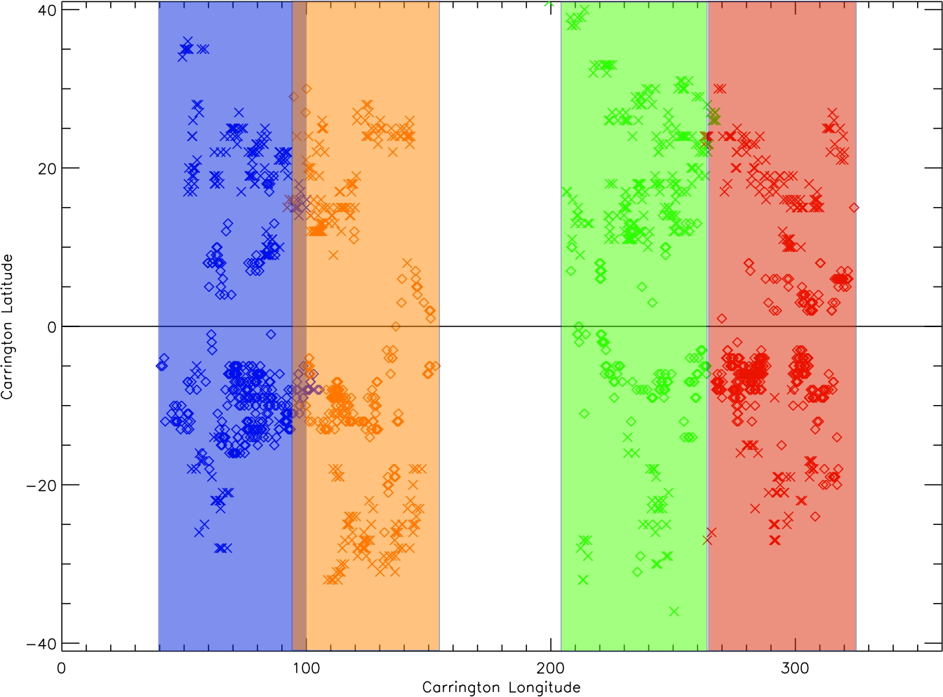
Figure 7: Sunspot longitudinal distribution. All sunspot groups affiliated with non-contemporaneous spot clusters between 2006 January 1 and 2011 April 11 are plotted with their Carrington latitudes against longitudes. Their longitudes have been shifted by $(\omega-\omega_{cr})(t-t_{0})$, where $t_{0}$ is 2006 January 1, as if they all emerged on $t_{0}$. The color scheme is used to distinguish spot clusters and has the same meaning as used in Fig. 5. Within each spot cluster, sunspot groups emerging before DOY 998 (2008 September 24) are plotted with “$\diamond$”, those emerging after DOY 998 are plotted with “$\times$”. Each cluster is further distinguished with colored transparent rectangles indicating the longitudinal range of the cluster. The solid horizontal line shows the equator.

Fig. 5 also reveals that active longitudes on the sun persist regardless of solar cycle or latitude. Fig. 7 shows the sunspot groups of the four clusters as if they all emerged on DOY = 1 (2006 January 1). The Carrington longitudes of sunspots are shifted by the quantity $[\omega-\omega_{cr}](t_{0}-t)$ within each cluster; $t_{0}=$2006 January 1, and $t$ is the time of a sunspot emergence. The color scheme in the figure has the same meaning as those in Fig.5. To distinguish the (low latitude) sunspot groups emerging in the end of cycle 23 from the (high latitude) sunspot groups emerging in new cycle 24, the cycle 23 spots are represented by “$\diamond$” symbols while those of cycle 24 are represented by “$\times$” symbols. The four clusters of sunspots clearly occupied four distinct longitudinal bands, each of them spanning $\sim$60${\arcdeg}$ in longitude. Although spot groups emerging in the new cycle occupy higher latitudes than those in the old cycle, consistent with the general trend of the Butterfly diagram, there is no evident change in the distribution of longitudes between spots appearing in the old and the new activity cycles. Figure (7) shows that the longitudinal clustering survives, indicating that whatever underlying magnetic structure causes the longitudinal clumping is not destroyed by the emergence of a new activity cycle.

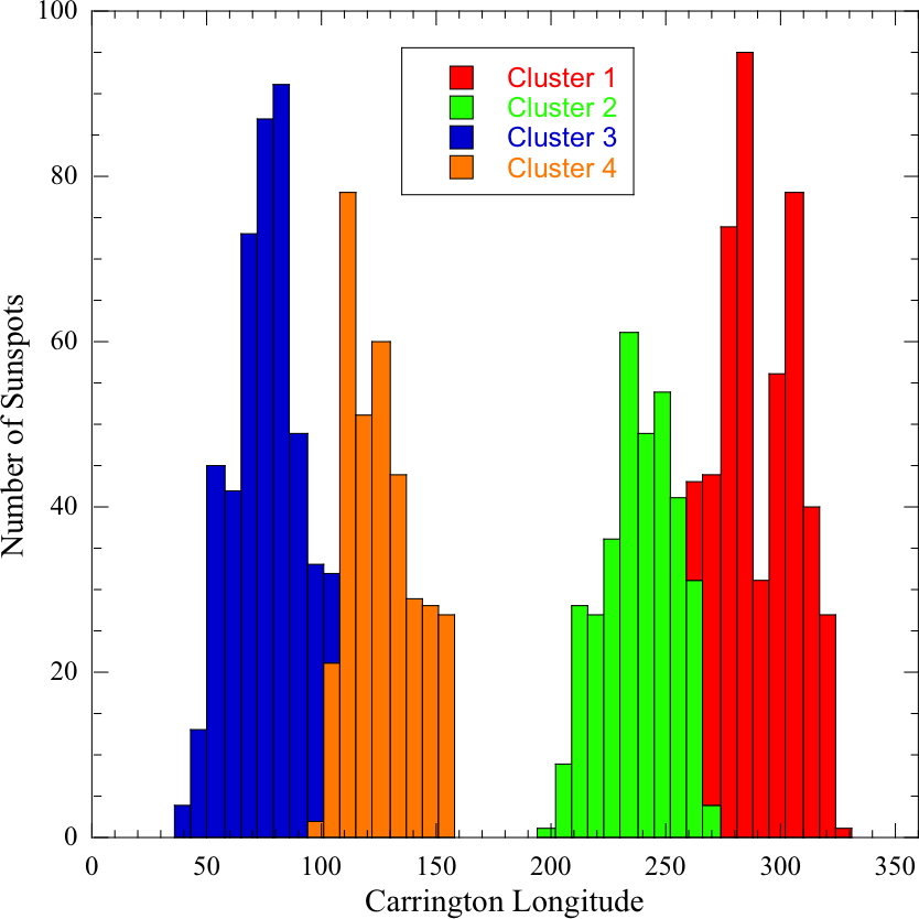
Figure 8: Sunspot longitudinal histogram. The sunspot longitudes have been shifted as in Figure 7, as if all sunspots emerged on 2006 January 1.

Fig. 8 further demonstrates the distribution of the sunspot longitudes within the four clusters, again plotted as if the spots all emerged on DOY =1 (2006 January 1). The distributions are clearly non-uniform, with preferred bands centered at roughly $90^{\circ}$ for the cluster pair 3 & 4 and $270^{\circ}$ for the cluster pair 1 & 2, respectively. Both bands have longitudinal range $\sim 100^{\circ}$. The centers of the two massively occupied longitudinal bands are separated by $\sim 180^{\circ}$.

6 Summary

We use EUV images from a $>5$ year (2006 January 1 and 2011 April 15) period around the recent solar activity minimum to identify long-lived coronal streamers. Comparing coronal streamers on Limb Synoptic Maps with photospheric sunspot records, we find that:

1. The EUV coronal streamers persist for many solar rotations and are non-randomly distributed in time and/or solar longitude. These long-lived structures are best detected on full coronal Limb Synoptic Maps.

2. The long-lived, large-scale coronal streamers on Limb Synoptic Maps reflect non-random longitudinal distributions of photospheric sunspot groups. They are long-lived because they are sustained by sunspot groups emerging in the vicinity of a longitude, but at different times on the sun.

3. Sunspots emerge clustered in longitude-time space. Lifetimes of these spot clusters are comparable to the 5-year time coverage of the current study. More than 75% of numbered sunspots in the period of study are members of these four spot clusters.

4. Sunspot clusters straddle the boundary between activity cycles 23 and 24.

5. Members of spot clusters share common rotation rates which are faster by $\sim$5% than both the surface and the bottom of the convection zone. The implication is that members of spot clusters are rooted in the convection zone.

6. The four spot clusters contain sunspots from both hemispheres at all latitudes. Heavily occupied longitudinal regions are characterized with two meridional bands each $\sim$100$\arcdeg$ wide and separated by $\sim$180$\arcdeg$.

Table 1: Properties of Non-contemporaneous Sunspot Clusters

Cluster	Time Duration	Carrington	Carrington	Sidereal Rate [∘day-1]		Synodic Period [days]
		$\bar{B}$	$\lambda_{0}(t_{0}=0)$	$\omega$    (nHz)	$\omega(\bar{B})$	P($\omega$)
1 (471)	2006/01/01 to 2011/04/15	$~{}8^{\circ}$	$291.4^{\circ}$	14.43 (464)	13.73	26.77
2 (356)	2006/01/01 to 2011/04/15	$15^{\circ}$	$238.1^{\circ}$	14.43 (464)	13.64	26.78
3 (440)	2006/01/07 to 2011/04/10	$11^{\circ}$	$~{}74.4^{\circ}$	14.38 (462)	13.69	26.88
4 (334)	2006/02/10 to 2011/04/08	$13^{\circ}$	$120.9^{\circ}$	14.38 (462)	13.67	26.87

Figure 2: Modeling a Polar Sinusoidal Streamer on a LSM. Sunspots and bright plage regions are outlined by contours. White dotted sinusoidal curves are calculated with Equations (1) and (4.1) given the latitudes $\delta=-65^{\circ}$. Numbers of curves correspond to sunspot groups marked with NOAA numbers. They shares the same rotation rates and phases as those numbered sunspots, and following a PSS. Each sinusoidal curve is plotted for 2 rotational periods.

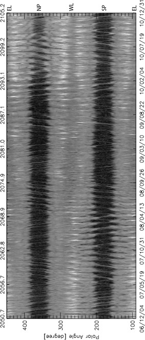
Figure 3:

Fig. 3 Coronal Full Limb Synoptic Map (LSM) made with EUVI 195/STEREO A images taken between December 2006 and December 2010. The full limb emissions are extracted between solar altitudes 1.045 and 1.055 R_☉. The horizontal axis represents time from past to future (lower horizontal axis), and Carrington rotation numbers (upper horizontal axis). The vertical direction represents the polar angle around the solar limb with $0^{\circ}$ (and $360^{\circ}$) being the north pole (NP), $90^{\circ}$ the east limb (EL), $180^{\circ}$ the south pole (SP) and $270^{\circ}$ the west limb (WL). The polar angle is plotted beyond the 0$\arcdeg$ to 360$\arcdeg$ range to present both polar regions without interruption.

References

- Altrock (2003) Altrock, R. C. 2003, Sol. Phys., 213, 23
- Antonucci & Svalgaard (1974a) Antonucci, E., & Svalgaard, L. 1974, Sol. Phys., 34, 3
- Antonucci & Svalgaard (1974b) Antonucci, E., & Svalgaard, L. 1974, Sol. Phys., 36, 115
- Aschwanden et al. (2007) Aschwanden, M. J., Winebarger, A., Tsiklauri, D., & Peter, H. 2007, ApJ, 659, 1673
- Babcock (1961) Babcock, H. W. 1961, ApJ, 133, 572
- Badalyan (2010) Badalyan, O. G. 2010, New Astronomy, 15, 135
- Bai (1987) Bai, T. 1987, ApJ, 314, 795
- Berdyugina & Tuominen (1998) Berdyugina, S. V., & Tuominen, I. 1998, A&A, 336, L25
- Berdyugina & Usoskin (2003) Berdyugina, S. V., & Usoskin, I. G. 2003, A&A, 405, 1121
- Beck (2000) Beck, J. G. 2000, Sol. Phys., 191, 47
- Berdyugina et al. (2006) Berdyugina, S. V., Moss, D., Sokoloff, D., & Usoskin, I. G. 2006, A&A, 445, 703
- Bogart (1982) Bogart, R. -S. 1982, Sol. Phys., 76, 155
- Brouwer & Zwaan (1990) Brouwer, M. P., & Zwaan, C. 1990, Sol. Phys., 129, 221
- Charbonneau (2010) Charbonneau, P. 2010, Living Reviews in Solar Physics, 7, 3
- Delaboudinière et al. (1995) Delaboudinière, J.-P., et al. 1995, Sol. Phys., 162, 291
- Devore et al. (1984) Devore, C. R., Boris, J. P., & Sheeley, N. R., Jr. 1984, Sol. Phys., 92, 1
- Dikpati & Charbonneau (1999) Dikpati, M., & Charbonneau, P. 1999, ApJ, 518, 508
- Dikpati & Gilman (2005) Dikpati, M., & Gilman, P. A. 2005, ApJ, 635, L193
- Domingo et al. (1995) Domingo, V., Fleck, B., & Poland, A. I. 1995, Sol. Phys., 162, 1
- D’Silva & Choudhuri (1993) D’Silva, S., & Choudhuri, A. R. 1993, A&A, 272, 621
- Fisher & Sime (1984) Fisher, R., & Sime, D. G. 1984, ApJ, 287, 959
- Foukal & Jokipii (1975) Foukal, P., & Jokipii, J. R. 1975, ApJ, 199, L71
- Gaizauskas et al. (1983) Gaizauskas, V., Harvey, K. L., Harvey, J. W., & Zwaan, C. 1983, ApJ, 265, 1056
- Gaizauskas et al. (1994) Gaizauskas, V., Harvey, K. L., & Proulx, M. 1994, ApJ, 422, 883
- Gaizauskas et al. (1998) Gaizauskas, V., Mandrini, C. H., Demoulin, P., Luoni, M. L., & Rovira, M. G. 1998, A&A, 332, 353
- Hale et al. (1919) Hale, G. E., Ellerman, F., Nicholson, S. B., & Joy, A. H. 1919, ApJ, 49, 153
- Hathaway (1996) Hathaway, D. H. 1996, ApJ, 460, 1027
- Hathaway & Rightmire (2010) Hathaway, D. H., & Rightmire, L. 2010, Science, 327, 1350
- Hara (2009) Hara, H. 2009, ApJ, 697, 980
- Howard & Harvey (1970) Howard, R., & Harvey, J. 1970, Sol. Phys., 12, 23
- Howard & Labonte (1980) Howard, R., & Labonte, B. J. 1980, ApJ, 239, L33
- Howard et al. (2008) Howard, R. A., et al. 2008, Space Science Reviews, 136, 67
- Howe et al. (2006) Howe, R., Komm, R., Hill, F., Ulrich, R., Haber, D. A., Hindman, B. W., Schou, J., & Thompson, M. J. 2006, Sol. Phys., 235, 1
- Insley et al. (1995) Insley, J. E., Moore, V., & Harrison, R. A. 1995, Sol. Phys., 160, 1
- Kaiser et al. (2008) Kaiser, M. L., Kucera, T. A., Davila, J. M., St. Cyr, O. C., Guhathakurta, M., & Christian, E. 2008, Space Science Reviews, 136, 5
- Leighton (1969) Leighton, R. B. 1969, ApJ, 156, 1
- Li et al. (1998) Li, J., Raymond, J. C., Acton, L. W., Kohl, J. L., Romoli, M., Noci, G., & Naletto, G. 1998, ApJ, 506, 431
- Li et al. (2000) Li, J., Jewitt, D., & LaBonte, B. 2000, ApJ, 539, L67
- Li et al. (2002) Li, J., LaBonte, B., Acton, L., & Slater, G. 2002, ApJ, 565, 1289
- Li et al. (2011) Li, K. J., Shi, X. J., Liang, H. F., Zhan, L. S., Xie, J. L., & Feng, W. 2011, ApJ, 730, 49
- Newton & Nunn (1951) Newton, H.W., and Nuun, M.L., 1951, MNRAS, 111, 413
- Olemskoy & Kitchatinov (2009) Olemskoy, S. V., & Kitchatinov, L. L. 2009, Geomagnetism and Aeronomy/Geomagnetizm i Aeronomiia, 49, 866
- Rempel (2007) Rempel, M. 2007, ApJ, 655, 651
- Rodriguez Taboada & Gil Moreno (1993) Rodriguez Taboada, R. E., & Gil Moreno, G. 1993, Sol. Phys., 144, 399
- Schuessler (1981) Schuessler, M. 1981, A&A, 94, L17
- Sheeley & Devore (1986) Sheeley, N. R., Jr., & Devore, C. R. 1986, Sol. Phys., 104, 425
- Sheeley et al. (1989) Sheeley, N. R., Wang, Y.-M., & Harvey, J. W. 1989, Sol. Phys., 119, 323
- Shelke & Shelke (1989) Shelke, R. N., & Shelke, J. N. 1989, Sol. Phys., 123, 69
- Sime et al. (1989) Sime, D. G., Fisher, R. R., & Altrock, R. C. 1989, ApJ, 336, 454
- Stix (1971) Stix, M. 1971, A&A, 13, 203
- Sýkora (1971) Sýkora, J. 1971, Sol. Phys., 18, 72
- Thompson et al. (1996) Thompson, M. J., et al. 1996, Science, 272, 1300
- Thompson (2006) Thompson, W. T. 2006, A&A, 449, 791
- Thompson & Wei (2010) Thompson, W. T., & Wei, K. 2010, Sol. Phys., 261, 215
- Tsuneta et al. (1991) Tsuneta, S., et al. 1991, Sol. Phys., 136, 37
- van Driel-Gesztelyi et al. (2003) van Driel-Gesztelyi, L., Démoulin, P., Mandrini, C. H., Harra, L., & Klimchuk, J. A. 2003, ApJ, 586, 579
- Vitinskij (1969) Vitinskij, J. I. 1969, Sol. Phys., 7, 210
- Vorontsov et al. (2002) Vorontsov, S. V., Christensen-Dalsgaard, J., Schou, J., Strakhov, V. N., & Thompson, M. J. 2002, Science, 296, 101
- Wang et al. (1988) Wang, Y.-M., Sheeley, N. R., Jr., Nash, A. G., & Shampine, L. R. 1988, ApJ, 327, 427
- Wang et al. (1991) Wang, Y.-M., Sheeley, N. R., Jr., & Nash, A. G. 1991, ApJ, 383, 431
- Wang & Sheeley (1993) Wang, Y.-M., & Sheeley, N. R., Jr. 1993, ApJ, 414, 916
- Wang et al. (2002) Wang, Y.-M., Lean, J., & Sheeley, N. R., Jr. 2002, ApJ, 577, L53
- Wöhl et al. (2010) Wöhl, H., Brajša, R., Hanslmeier, A., & Gissot, S. F. 2010, A&A, 520, A29
- Yoshimura (1981) Yoshimura, H. 1981, ApJ, 247, 1102
- Zhang et al. (2011) Zhang, L., Mursula, K., Usoskin, I., & Wang, H. 2011, Journal of Atmospheric and Solar-Terrestrial Physics, 73, 258
- Zhao & Kosovichev (2004) Zhao, J., & Kosovichev, A. G. 2004, ApJ, 603, 776