Coronal Shock Waves, EUV waves, and their Relation to CMEs. II. Modeling MHD Shock Wave Propagation Along the Solar Surface, Using Nonlinear Geometrical Acoustics

Abstract

We model the propagation of a coronal shock wave, using nonlinear geometrical acoustics. The method is based on the Wentzel–Kramers–Brillouin (WKB) approach and takes into account the main properties of nonlinear waves: i) dependence of the wave front velocity on the wave amplitude, ii) nonlinear dissipation of the wave energy, and iii) progressive increase in the duration of solitary shock waves. We address the method in detail and present results of the modeling of the propagation of shock-associated extreme-ultraviolet (EUV) waves as well as Moreton waves along the solar surface in the simplest solar corona model. The calculations reveal deceleration and lengthening of the waves. In contrast, waves considered in the linear approximation keep their length unchanged and slightly accelerate.

1 Introduction

Many solar eruptive events appear to initiate magnetohydrodynamic (MHD) waves in the corona. This conjecture is supported by observations of their manifestations. First, these are waves visible in chromospheric spectral lines. For several decades, Moreton waves have been known [Moreton and Ramsey (1960)] observed in the H$\alpha$ line. Uchida68 proposed that a Moreton wave represented the chromospheric trail of a coronal fast-mode wave. More recent studies show the possible coronal nature of Moreton waves (see, e.g., Balasubramaniam07). Similar phenomena are propagating waves observed in the He I 10830 $\mathrm{\AA}$ line (see, e.g., Vrsnak02b; Gilbert04). Second, type II radio bursts are considered to be signatures of coronal shock waves propagating upwards in the corona [Uchida (1960)]. Furthermore, presumable signatures of coronal waves can be observed in soft X-rays (Narukage02; Khan02; Hudson03; Warmuth05), microwaves (Warmuth04a; White05), and metric radio-wavelengths (Vrsnak05).

Other phenomena that can be manifestations of MHD waves are large-scale wave-like disturbances discovered in 1998 with the Extreme-ultraviolet Imaging Telescope (EIT) and referred to as “EIT waves” or “extreme-ultraviolet (EUV) waves”. This term appears to include phenomena having different physical nature and therefore various morphological and dynamical properties. For more details, we refer the reader to the Introduction of an accompanying paper [Grechnev et al. (2011b)]. Note here that describing EUV waves in terms of fast-mode MHD waves seems to be possible and correct for those cases when we really deal with “wave” phenomena. Just this class of EUV transients is the subject of our consideration.

Thus, fast-mode MHD waves are responsible for a number of solar transients and it is important to describe their propagation through the corona. But some questions about modeling the waves remain.

In his original approach, Uchida68 modeled a coronal disturbance as a linear and short fast-mode MHD wave propagating from a point source. To calculate a dome-like surface of the wave front and find the position of a Moreton wave (as an intersection line of the dome and the solar surface), he used the linear geometric acoustics [the Wentzel–Kramers–Brillouin (WKB) approach]. Some recent studies (see, e.g., Wang00; Patsourakos09) also used the same approach under the assumption of a linear disturbance. In this case, the disturbance moves along rays, which curve into regions of a reduced Alfvén speed. This results in the appearance of wave “imprints” (e.g., Moreton waves) running along the spherical solar surface. Note that in the linear approximation the amplitude and duration of the wave do not affect the shape of the wave front and the speed of its motion along the rays. Neither amplitude nor duration of the wave were calculated in the mentioned papers; the geometry of the propagation was their only interest. Henceforth in the paper, we consider the wave amplitude to be the perturbation magnitude of the plasma velocity in the wave.

Uchida’s model of a linear MHD wave has demonstrated the possibility to describe Moreton waves in these terms. Later papers by Uchida with collaborators (Uchida73; Uchida74) and recent papers (Wang00; Patsourakos09), in which the coronal magnetic field was calculated from photospheric magnetograms, provided a more accurate quantitative description of Moreton and EUV waves in terms of the linear model.

However, the linear model predicts acceleration of Moreton and EUV waves, whereas observations show their systematic deceleration (Warmuth et al. 2001; 2004a). Also, it is often pointed out by many authors that the speeds of coronal waves sometimes well exceed the fast-mode ones (Narukage02; Vrsnak02a; Narukage04; Warmuth04b; Muhr10). These facts suggest that the linear approximation does not always correctly describe the propagation of those waves. Probably, the disturbance responsible for the transients listed above is nonlinear and most likely is a shock wave.

Studies of the propagation of shock waves meet difficulties due to their nonlinearity. Analytic methods to describe the propagation of shock waves are approximate and often describe the behavior of some extreme classes of nonlinear waves (e.g., very strong self-similar waves, or weak waves, etc.). The present paper is devoted to the case of a weak shock wave that appears to be the most acceptable (see, e.g., Warmuth04b; Vrsnak02a). We do not discuss the appearance of a shock wave. Vrsnak00 approximately described this process, based on an analogy with an accelerating flat piston. The cases of cylindrical and spherical pistons were analyzed by Zic08. Temmer09 demonstrated how one could describe the kinematics of a Moreton wave by using the solution of a simple wave without a discontinuity. In our study, we assume that a fast-mode shock wave of moderate intensity appears during a solar eruption on the periphery of an active region and decays to a weak shock when traveling in the corona. The wave manifests as a Moreton wave and an EUV wave on the solar disk. We calculate the propagation of the shock wave in terms of the WKB approach taking into account nonlinear effects.

Such a method in its generally accepted variant involves two independent procedures. In the first one, ray trajectories corresponding to the linear approximation as well as cross sections of ray tubes are calculated. So, the influence of the finite wave amplitude on the wave front shape and ray trajectories is ignored because in linear acoustics the propagation velocities of disturbances are equal to the undisturbed sound speed regardless of their amplitude. In the second procedure, the nonlinear variation of the wave amplitude and duration are computed along the linear rays obtained. Such a non-self-consistent approach is fairly useful in some cases, however, nonlinear effects altering the ray pattern and the wave velocity disappear completely. Therefore, we develop another method, which allows us to consider self-consistently wave propagation and the nonlinear variation of wave characteristics.

The method is described in Section S-method. In Section S-modeling we formulate the problem and present results of the analytic propagation model of Moreton and EUV waves along the solar surface. Section S-conclusion contains concluding remarks about the method and the results. We note that those who are not interested in the mathematical details of the method can read Section 3 without going through Section 2.

2 Method

S-method

The method of nonlinear geometrical acoustics is based on the method of linear geometrical acoustics and allows one to calculate the propagation of disturbances with small (but finite) amplitudes through an inhomogeneous medium. The linear geometrical acoustics is known to be a method to calculate linear disturbances in the ray approximation (see, e.g., Landau87). In this approximation, a solution is found in the form of $A\left(\mathbf{r},t\right)e^{i\Psi\left(\mathbf{r},t\right)}$ where $A\left(\mathbf{r},t\right)$ is the wave amplitude, and $\Psi\left(\mathbf{r},t\right)$ is the eikonal, both depending on coordinates and time. By substituting this representation for wave perturbations into the system of linearized equations of ideal magnetohydrodynamics, one can obtain a Hamilton–Jacobi partial differential equation for the eikonal of fast and slow magnetosonic waves:

$$\frac{\partial\Psi}{\partial t}+\left(\mathbf{V}\mathrm{grad}\Psi\right)+a\left|\mathrm{grad}\Psi\right|=0,$$

where $\mathbf{V}$ is the undisturbed plasma flow velocity (e.g., the solar wind velocity), and $a$ is the magnetosonic speed in plasma. Solving the equation with the method of characteristics gives a system of ray equations, which in spherical coordinates $(r,\theta,\varphi)$ takes the form Uralova and Uralov (1994)

$$\frac{dr}{dt} = V_{r}+a\frac{k_{r}}{k}+k\frac{\partial a}{\partial k_{r}},$$

$$r\frac{d\theta}{dt} = a\frac{k_{\theta}}{k}+k\frac{\partial a}{\partial k_{\theta}},$$

$$r\sin\theta\frac{d\varphi}{dt} = a\frac{k_{\varphi}}{k}+k\frac{\partial a}{\partial k_{\varphi}},$$ (1)

$$\frac{dk_{r}}{dt} = -\frac{\partial V_{r}}{\partial r}k_{r}-\frac{\partial a}{\partial r}k+\frac{a}{kr}\left(k_{\theta}^{2}+k_{\varphi}^{2}\right),$$

$$r\frac{dk_{\theta}}{dt} = -\frac{\partial V_{r}}{\partial\theta}k_{r}-\frac{\partial a}{\partial\theta}k+\frac{a}{k}k_{\varphi}^{2}\cot\theta-k_{\theta}\frac{dr}{dt},$$

$$r\sin\theta\frac{dk_{\varphi}}{dt} = -\frac{\partial V_{r}}{\partial\varphi}k_{r}-\frac{\partial a}{\partial\varphi}k-\sin\theta k_{\varphi}\frac{dr}{dt}-k_{\varphi}r\cos\theta\frac{d\theta}{dt},$$

where $k_{r,\theta,\varphi}$ are the components of the wave vector $\mathbf{k}=\mathrm{grad}\Psi$, and $k$ is its magnitude. The system of equations (E-ray_eq_system) corresponds to the case of a medium in steady-state, where only the radial component $V_{r}$ of the undisturbed plasma flow exists. By integrating the system (E-ray_eq_system), one can determine the wave front shape.

This approach has been used for modeling coronal fast-mode MHD waves Uchida (1968); Wang (2000), with only the ray pattern being calculated. However, it is essential not only to find the wave geometry, but also to calculate the wave intensity. The geometrical acoustics allows the wave amplitude variation to be calculated.

In the linear geometrical acoustics, the energy flux of a disturbance traveling in a stationary medium with group velocity $\mathbf{q}_{0}$ is directed along the rays, and its magnitude is conserved within a ray tube Blokhintsev (1981), $\mathrm{div}(\Delta\varepsilon\mathbf{q}_{0})=0$, where $\Delta\varepsilon$ is the average density of the disturbance energy. In a medium moving at a velocity of $\mathbf{V}$, we have to take into account the fact that the wave front phase velocity varies as $q_{n}=V_{n}+a$, with the $n$ index denoting the projection normal to the front. The conservation law in this case is $\mathrm{div}(\Delta\varepsilon\mathbf{q}\,q_{n}/a)=0$ Uralov (1982); Barnes (1992) where $\mathbf{q}=\mathbf{V}+\mathbf{q}_{0}$ is the group velocity in a moving medium. The average density of the disturbance energy is $\Delta\varepsilon=\rho\overline{\left(u^{2}+v^{2}\right)}$ where $\rho$ is the undisturbed plasma density, and $u,v$ are the plasma velocity components along the normal to the wave front and across it, respectively. Taking into account the relation between the plasma velocity components $\mu=v/u$ Kulikovsky and Lyubimov (2005), it is possible to relate the variation of the wave amplitude to the normal cross section $dS$ of the ray tube formed by a bundle of rays:

$$dSq\rho u^{2}\left(1+\mu^{2}\right)\frac{q_{n}}{a}=const.\ilabel{E-dS_{w}ave_{a}mp_{v}ariation}$$ (2)

Thus, the general approach to determine the wave amplitude in the ray method relies on calculating the cross section of the ray tube.

There are various techniques for calculating cross sections. They are discussed in KravtsovOrlov90. We calculate cross sections by using the Jacobian of the transformation to ray coordinates. The volume element $dW$ of the ray tube is expressed in terms of ray coordinates $(\eta_{1},\eta_{2},t)$ as

$$dW=dxdydz=r^{2}\sin\theta drd\theta d\varphi=r^{2}\sin\theta D\left(t\right)d\eta_{1}d\eta_{2}dt,$$

where $D(t)$ is the Jacobian of the transformation from spherical coordinates to ray ones. Then for the cross section of the ray tube, $dS$, we have

$$dS=\frac{dW}{d\sigma}=r^{2}\sin\theta\frac{D\left(t\right)}{q}d\eta_{1}d\eta_{2},$$

where $\sigma$ is the ray tube length. Substituting it into (E-dS_wave_amp_variation) yields

$$D\left(t\right)r^{2}\sin\theta\rho u^{2}\left(1+\mu^{2}\right)\frac{q_{n}}{a}=const.\ilabel{E-Jacob_{w}ave_{a}mp_{v}ariation}$$ (3)

To calculate the Jacobian, we use a method based on numerical integration of a so-called adjoint system of equations. This system consists of differential equations for the derivatives $\partial r/\partial\eta_{1,2}$, $\partial\theta/\partial\eta_{1,2}$, $\partial\varphi/\partial\eta_{1,2}$, $\partial k_{r}/\partial\eta_{1,2}$, $\partial k_{\theta}/\partial\eta_{1,2}$, $\partial k_{\varphi}/\partial\eta_{1,2}$ and is derived from (E-ray_eq_system) by differentiating the equations with respect to ray coordinates $\eta_{1}$ and $\eta_{2}$. Let the ray coordinates $\eta_{1}$ and $\eta_{2}$ be the angles defining the direction of the outgoing ray from a point source at the initial moment. Note that the ray coordinates do not need to be explicitly determined when the adjoint system is being derived. This becomes essential to specify the initial values for the desired functions. For the case considered, the adjoint system has the following form (in view of the symmetry about $\eta_{1}$ and $\eta_{2}$, instead of 12 equations we give only six for one variable $\eta$):

$$\frac{d}{dt}\left(\frac{\partial r}{\partial\eta}\right)=\frac{\partial V_{r}}{\partial\eta}+\frac{k_{r}}{k}\frac{\partial a}{\partial\eta}+\frac{a}{k}\frac{\partial k_{r}}{\partial\eta}-\frac{ak_{r}}{k^{2}}\frac{\partial k}{\partial\eta}+\frac{\partial a}{\partial k_{r}}\frac{\partial k}{\partial\eta}+k\frac{\partial}{\partial\eta}\left(\frac{\partial a}{\partial k_{r}}\right),$$

$$\frac{\partial r}{\partial\eta}\frac{d\theta}{dt}+r\frac{d}{dt}\left(\frac{\partial\theta}{\partial\eta}\right)=\frac{k_{\theta}}{k}\frac{\partial a}{\partial\eta}+\frac{a}{k}\frac{\partial k_{\theta}}{\partial\eta}-\frac{ak_{\theta}}{k^{2}}\frac{\partial k}{\partial\eta}+\frac{\partial a}{\partial k_{\theta}}\frac{\partial k}{\partial\eta}+k\frac{\partial}{\partial\eta}\left(\frac{\partial a}{\partial k_{\theta}}\right),$$

$$\frac{\partial r}{\partial\eta}\sin\theta\frac{d\varphi}{dt}+r\cos\theta\frac{\partial\theta}{\partial\eta}\frac{d\varphi}{dt}+r\sin\theta\frac{d}{dt}\left(\frac{\partial\varphi}{\partial\eta}\right)=\qquad\qquad\qquad\qquad\qquad\qquad$$

$$=\frac{\partial a}{\partial\eta}\frac{k_{\varphi}}{k}+\frac{a}{k}\frac{\partial k_{\varphi}}{\partial\eta}-\frac{ak_{\varphi}}{k^{2}}\frac{\partial k}{\partial\eta}+\frac{\partial a}{\partial k_{\varphi}}\frac{\partial k}{\partial\eta}+k\frac{\partial}{\partial\eta}\left(\frac{\partial a}{\partial k_{\varphi}}\right),$$

$$\frac{d}{dt}\left(\frac{\partial k_{r}}{\partial\eta}\right)=-\frac{\partial V_{r}}{\partial r}\frac{\partial k_{r}}{\partial\eta}-k_{r}\frac{\partial}{\partial\eta}\left(\frac{\partial V_{r}}{\partial r}\right)-\frac{\partial a}{\partial r}\frac{\partial k}{\partial\eta}-k\frac{\partial}{\partial\eta}\left(\frac{\partial a}{\partial r}\right)+\frac{\partial a}{\partial\eta}\frac{k_{\theta}^{2}+k_{\varphi}^{2}}{kr}-$$

$$-\frac{a}{k^{2}r}\left(k_{\theta}^{2}+k_{\varphi}^{2}\right)\frac{\partial k}{\partial\eta}-\frac{a\left(k_{\theta}^{2}+k_{\varphi}^{2}\right)}{kr^{2}}\frac{\partial r}{\partial\eta}+\frac{a}{kr}\left(2k_{\theta}\frac{\partial k_{\theta}}{\partial\eta}+2k_{\varphi}\frac{\partial k_{\varphi}}{\partial\eta}\right),$$

$$\frac{\partial r}{\partial\eta}\frac{dk_{\theta}}{dt}+r\frac{d}{dt}\left(\frac{\partial k_{\theta}}{\partial\eta}\right)=-\frac{\partial V_{r}}{\partial\theta}\frac{\partial k_{r}}{\partial\eta}-k_{r}\frac{\partial}{\partial\eta}\left(\frac{\partial V_{r}}{\partial\theta}\right)-\frac{\partial a}{\partial\theta}\frac{\partial k}{\partial\eta}-k\frac{\partial}{\partial\eta}\left(\frac{\partial a}{\partial\theta}\right)+$$

$$+\frac{\partial a}{\partial\eta}\frac{k_{\varphi}^{2}\cot\theta}{k}-\frac{ak_{\varphi}^{2}}{k^{2}}\cot\theta\frac{\partial k}{\partial\eta}+\frac{2ak_{\varphi}}{k}\cot\theta\frac{\partial k_{\varphi}}{\partial\eta}-\qquad\qquad\qquad\qquad$$

$$-\frac{ak_{\varphi}^{2}}{k\sin^{2}\theta}\frac{\partial\theta}{\partial\eta}-\frac{\partial k_{\theta}}{\partial\eta}\frac{dr}{dt}-k_{\theta}\frac{d}{dt}\left(\frac{\partial r}{\partial\eta}\right),$$ (4)

$$\frac{\partial r}{\partial\eta}\sin\theta\frac{dk_{\varphi}}{dt}+r\cos\theta\frac{\partial\theta}{\partial\eta}\frac{dk_{\varphi}}{dt}+r\sin\theta\frac{d}{dt}\left(\frac{\partial k_{\varphi}}{\partial\eta}\right)=\qquad\qquad\qquad\qquad\qquad\qquad$$

$$=-\frac{\partial V_{r}}{\partial\varphi}\frac{\partial k_{r}}{\partial\eta}-k_{r}\frac{\partial}{\partial\eta}\left(\frac{\partial V_{r}}{\partial\varphi}\right)-\frac{\partial a}{\partial\varphi}\frac{\partial k}{\partial\eta}-k\frac{\partial}{\partial\eta}\left(\frac{\partial a}{\partial\varphi}\right)-\cos\theta\frac{\partial\theta}{\partial\eta}k_{\varphi}\frac{dr}{dt}-$$

$$-\sin\theta\frac{\partial k_{\varphi}}{\partial\eta}\frac{dr}{dt}-\sin\theta k_{\varphi}\frac{d}{dt}\left(\frac{\partial r}{\partial\eta}\right)-\frac{\partial k_{\varphi}}{\partial\eta}r\cos\theta\frac{d\theta}{dt}-k_{\varphi}\frac{\partial r}{\partial\eta}\cos\theta\frac{d\theta}{dt}+$$

$$+k_{\varphi}r\sin\theta\frac{\partial\theta}{\partial\eta}\frac{d\theta}{dt}-k_{\varphi}r\cos\theta\frac{d}{dt}\left(\frac{\partial\theta}{\partial\eta}\right),$$

where

$$\frac{\partial V_{r}}{\partial\eta}=\sum\limits_{\alpha}\frac{\partial V_{r}}{\partial r_{\alpha}}\frac{\partial r_{\alpha}}{\partial\eta},\quad\frac{\partial a}{\partial\eta}=\sum\limits_{\alpha}\left(\frac{\partial a}{\partial r_{\alpha}}\frac{\partial r_{\alpha}}{\partial\eta}+\frac{\partial a}{\partial k_{\alpha}}\frac{\partial k_{\alpha}}{\partial\eta}\right),\quad\frac{\partial k}{\partial\eta}=\frac{1}{k}\sum\limits_{\alpha}k_{\alpha}\frac{\partial k_{\alpha}}{\partial\eta},$$

$$\frac{\partial}{\partial\eta}\left(\frac{\partial a}{\partial k_{\beta}}\right)=\sum\limits_{\alpha}\left(\frac{\partial}{\partial r_{\alpha}}\left(\frac{\partial a}{\partial k_{\beta}}\right)\frac{\partial r_{\alpha}}{\partial\eta}+\frac{\partial}{\partial k_{\alpha}}\left(\frac{\partial a}{\partial k_{\beta}}\right)\frac{\partial k_{\alpha}}{\partial\eta}\right),\qquad\qquad$$

$$\frac{\partial}{\partial\eta}\left(\frac{\partial a}{\partial r_{\beta}}\right)=\sum\limits_{\alpha}\left(\frac{\partial}{\partial r_{\alpha}}\left(\frac{\partial a}{\partial r_{\beta}}\right)\frac{\partial r_{\alpha}}{\partial\eta}+\frac{\partial}{\partial k_{\alpha}}\left(\frac{\partial a}{\partial r_{\beta}}\right)\frac{\partial k_{\alpha}}{\partial\eta}\right),\qquad\qquad$$

$$\frac{\partial}{\partial\eta}\left(\frac{\partial V_{r}}{\partial r_{\beta}}\right)=\sum\limits_{\alpha}\left(\frac{\partial}{\partial r_{\alpha}}\left(\frac{\partial V_{r}}{\partial r_{\beta}}\right)\frac{\partial r_{\alpha}}{\partial\eta}\right),\quad r_{\alpha,\beta}=\{r,\theta,\varphi\},\;\;k_{\alpha,\beta}=\{k_{r},k_{\theta},k_{\varphi}\}.$$

Thus, to calculate the propagation of a linear wave and its intensity, at first we have to integrate numerically the ray equations system (E-ray_eq_system) and adjoint system (E-eq_system_for_calc amp) and then determine the amplitude variations by means of (E-Jacob_wave_amp_variation).

A nonlinear flat disturbance in an ideal homogeneous medium is described by a simple wave solution and propagates at the supersonic speed determined by its amplitude Kulikovsky and Lyubimov (2005). A fast-mode simple-wave element with plasma velocity component $u$ normal to the front moves at $a+\kappa u$, where $\kappa=\left(1/a\right)\left(d\left(\rho a\right)/d\rho\right)$ is the numerical coefficient depending both on the plasma beta and the angle between the wave vector and the magnetic field. We do not give here the bulky explicit expression for $\kappa$. We only note that values of $\kappa$ are restricted by the limits: $1/2\leq\kappa\leq 3/2$. The fact that each simple-wave element travels at its own speed causes wave profile deformation and the appearance of a discontinuity. If a moderate amplitude simple wave has a triangular profile before the discontinuity appears, it will take the shape of the right-angled triangle after the discontinuity forms, with the discontinuity being the leading edge of the disturbance. Note that any nonlinear disturbance profile of a finite duration tends asymptotically to this shape. Let $U_{sh}$ be the jump of the plasma velocity component $u$ in the discontinuity. Then, in the nonlinear geometrical acoustics approximation, the discontinuity moves at a speed of $a+\kappa U_{sh}/2$. Taking into account this increase in the wave front speed in the ray equations, we are able to correctly describe the propagation of weak shock waves. Then the ray equation system (E-ray_eq_system) becomes Uralova and Uralov (1994)

$$\frac{dr}{dt} = V_{r}+\left(a+\frac{\kappa U_{sh}}{2}\right)\frac{k_{r}}{k}+k\frac{\partial a}{\partial k_{r}},$$

$$r\frac{d\theta}{dt} = \left(a+\frac{\kappa U_{sh}}{2}\right)\frac{k_{\theta}}{k}+k\frac{\partial a}{\partial k_{\theta}},$$

$$r\sin\theta\frac{d\varphi}{dt} = \left(a+\frac{\kappa U_{sh}}{2}\right)\frac{k_{\varphi}}{k}+k\frac{\partial a}{\partial k_{\varphi}},$$ (5)

$$\frac{dk_{r}}{dt} = -\frac{\partial V_{r}}{\partial r}k_{r}-\frac{\partial a}{\partial r}k+\frac{a}{kr}\left(k_{\theta}^{2}+k_{\varphi}^{2}\right),$$

$$r\frac{dk_{\theta}}{dt} = -\frac{\partial V_{r}}{\partial\theta}k_{r}-\frac{\partial a}{\partial\theta}k+\frac{a}{k}k_{\varphi}^{2}\cot\theta-k_{\theta}\frac{dr}{dt},$$

$$r\sin\theta\frac{dk_{\varphi}}{dt} = -\frac{\partial V_{r}}{\partial\varphi}k_{r}-\frac{\partial a}{\partial\varphi}k-\sin\theta k_{\varphi}\frac{dr}{dt}-k_{\varphi}r\cos\theta\frac{d\theta}{dt}.$$

The generally accepted method of nonlinear geometrical acoustics ignores the additional term $\kappa U_{sh}/2$ as it is small. However, it is the term that is responsible for wave deceleration due to the amplitude damping. Besides, estimations within the framework of the perturbation theory suggest that the ray pattern variation due to nonlinearity is a correction of the same order of magnitude as the nonlinear variation of the wave amplitude is. It is therefore important to take this into account in the nonlinear geometrical acoustics approximation.

Ray equation system (E-nonlin_ray_eq_system) is not closed now because it includes the wave amplitude. In the linear approximation, an amplitude variation can be determined from (E-Jacob_wave_amp_variation). The nonlinear wave amplitude undergoes additional damping associated with energy dissipation in the discontinuity. As the amplitude, we take the value of the jump $U_{sh}$. Variations of amplitude $U_{sh}$ and duration $T_{sh}$ of a weak shock wave having a triangular compression phase may be calculated as Uralov (1982)

$$U_{sh}=u_{1}\left(1+\frac{\tau_{1}}{T_{\ast}}\right)^{-1/2},\;\;T_{sh}=T_{\ast}\left(1+\frac{\tau_{1}}{T_{\ast}}\right)^{1/2},\;\;\frac{d\tau_{1}}{dt}=\frac{\kappa u_{1}}{q_{n}}\ilabel{E-damping_{l}aws}$$ (6)

where $\tau_{1}$ is the duration increment of the simple wave with an amplitude of $u_{1}$; $T_{\ast}$ is the initial duration of the disturbance. Note that the laws (E-damping_laws) of the weak shock wave damping are derived by using values of the amplitude and duration of a simple wave, from which the discontinuity forms. The value of $u_{1}$ can be determined from the expression similar to (E-Jacob_wave_amp_variation).

Thus, solving numerically of 19 ordinary differential equations (E-nonlin_ray_eq_system), (E-eq_system_for_calc amp), and (E-damping_laws) enables us to compute propagation of a weak shock wave in an inhomogeneous medium, its amplitude and duration.

3 Analytical Modeling of Wave Propagation

S-modeling

In this section, we employ the nonlinear geometrical acoustics method to describe the propagation of large-scale wave-like transients, namely EUV and Moreton waves. With respect to “EUV wave” phenomena, we address only those disturbances that are associated with a fast-mode MHD shock wave.

To calculate the propagation of a shock wave, we have to specify the solar corona model as well as position and parameters of the shock wave at the initial moment. We use a simple hydrostatic corona model to demonstrate the main particularities of the method and compare results with those obtained in the linear approximation. The corona is considered to be isothermal with temperature $T=1.5\times 10^{6}$ K and sound speed $c=181$ km s^-1. The plasma density is distributed in accordance with the barometric law (for details see, e.g., Mann99):

$$n(r)=n_{0}\;\mathrm{exp}\left(\frac{R_{\odot}}{H}\left(\frac{R_{\odot}}{r}-1\right)\right),\ilabel{E-barometric_{d}ensity_{l}aw}$$ (7)

where $n_{0}=n(R_{\odot})=3\times 10^{8}$ cm^-3 is the density at the base of the corona, $R_{\odot}$ the solar radius, $H=2R_{gas}T/\widetilde{m}M_{H}g_{\odot}\approx 70$ Mm the density scale height, $g_{\odot}$ the acceleration of gravity on the solar surface, $M_{H}$ the molar mass of hydrogen, $\widetilde{m}=1.27$ the average atomic weight of an ion, and $R_{gas}$ the gas constant. Let us assume that we have a magnetic field with only a radial component (for details see, e.g., Mann03):

$$B_{r}=\pm B_{0}\left(\frac{R_{\odot}}{r}\right)^{2},\ilabel{E-magn_{f}ield}$$ (8)

where $B_{0}=2.3$ G is its value at the base of the corona. The sign in (E-magn_field) depends on the solar hemisphere, but it is not meaningful here. The same model was applied by Uchida68.

Figure 1.: The Alfvén speed distribution in the solar corona model (E-barometric_density_law), (E-magn_field).F-alfven˙velocity

In the corona model (E-barometric_density_law) and (E-magn_field), the Alfvén speed increases with height, peaking at $R_{\odot}^{2}/4H=2.43\;R_{\odot}$ (Figure F-alfven_velocity). Refraction makes ray trajectories curved towards regions of the lower Alfvén speed. The solar corona has therefore waveguide properties. A portion of the wave energy flux is captured by the coronal waveguide and propagates along the solar surface, giving rise to an EUV and Moreton wave. In the treatment used, the EUV front is observable due to the plasma compression produced by the coronal shock wave. Since the plasma density decreases rapidly with height, a plasma layer near the solar surface contributes substantially to the EUV front emission. The layer thickness is about the density scale height $H$. So, to estimate the EUV front position, we have to find the intersection line of the calculated shock front and a spherical surface of radius $\lesssim(R_{\odot}+H)$. The Moreton wave corresponds to the chromospheric trail of the coronal shock wave, i.e. it can be found at the intersection line of the shock front and the upper chromosphere.

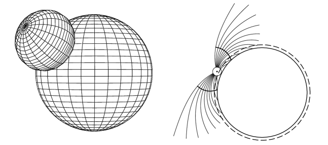
Figure 2.: Propagation of a coronal shock wave as seen in a 3D image (left) and a 2D cross section with ray trajectories (right). The solid arcs drawn across the rays represent shock wave fronts. The dashed line marks a height of 60 Mm above the solar surface. The wave front velocity along this line corresponds to the velocity of an EUV wave. The wave source height is 80 Mm.F-wave˙prop

For modeling, it is important to assign the initial characteristics of the shock wave and its start position. We have to specify the initial duration (or length) of the wave and its initial amplitude on some surface. In this study, these values are given according to the strong point-like explosion theory. The wave source located at a height of 80 Mm is characterized by the energy $\tilde{\varepsilon}$ whose release produces the shock wave. When the wave covers a distance of $\Lambda=(\tilde{\varepsilon}/\rho_{\ast}a_{\ast}^{2})^{1/3}$, with $\rho_{\ast}$ and $a_{\ast}$ being respectively the plasma density and the fast-mode speed at the explosion point, the compression phase profile of the wave is assumed to be triangular. The compression phase length is equal to $\Lambda$ and the amplitude is $\chi a_{\ast}$, with $\chi$ being a coefficient of the order of unity. In this paper, we employ a value $\chi=1$ except for the calculations given in Figure F-EUV_decay. The initial duration of the compression phase is supposed to be equal to $T_{\ast}=\Lambda(\mathbf{k})/a_{\ast}(\mathbf{k})$. We believe that a shock wave arises on the periphery of an active region located within the explosion cavity $\Lambda$. This manner to assign initial values does not rely on the specific mechanism of the wave initiation. It is essential only that the energy release producing a shock wave is impulsive. For instance, a wave can be produced by a compact piston acting for a short term (an abruptly accelerating filament and its magnetic envelope).

Figures F-wave_prop–F-EUV_decay present the results of our modeling. Figure F-wave_prop illustrates a 3D image of the shock wave front and the respective 2D section including ray trajectories. The rays go out from the initial surface of size $\Lambda$. The wave front gets inclined over the solar surface, with its inclination increasing in time.

Figure F-wave_speed_vs_energy shows the distance–time plots of EUV waves (a) as well as the time plots of their velocities (b) along the surface 60 Mm (relative to the solar surface). The curves are given for different values of the wave source energy $\tilde{\varepsilon}$ or different values of the initial shock wave length, as follows from $\Lambda=(\tilde{\varepsilon}/\rho_{\ast}a_{\ast}^{2})^{1/3}$. The EUV wave velocity decreases appreciably due to the nonlinear damping of the coronal wave amplitude. After the amplitude has substantially decreased, the shock wave propagates as a linear one. Having reached its minimum, the wave velocity slightly increases. This is due to the shock front inclination over the solar surface that becomes more and more significant with time and associated with the waveguide properties of the lower quiet Sun’s corona. The larger the wave front inclination, the higher the Moreton and EUV wave velocity. Note that calculated Moreton and EUV wave acceleration must be difficult to observe since it occurs when the wave amplitude becomes low (see Figure F-EUV_wave_amplitudes).

                                      a                                           b

Figure 3.: The distance–time plot of EUV waves (a) and the time evolution of their velocities (b) along the surface at 60 Mm height for different energies $\tilde{\varepsilon}$ specified in panel b. The lowest (dotted) line represents the linear EUV wave.F-wave˙speed˙vs˙energy

            a                                           b

Figure 4.: The kinematic plots of a Moreton wave (thick) and an EUV wave (thin), which are produced by a single coronal wave in the linear (dotted) and nonlinear (solid) consideration.F-EUV˙Moreton˙wave˙speeds

Figure F-EUV_Moreton_wave_speeds shows positions (a) counted along the surface and velocities (b) of a Moreton wave (thick lines) and an EUV wave (thin lines), which are produced by a single coronal wave. The dotted lines correspond to a linear coronal wave and the solid lines are for a shock one. The linear Moreton wave velocity is lower because the Alfvén speed at the corona base is smaller than that at a height of $60$ Mm. Note that a Moreton wave decelerates even in the linear case. This fact is associated with the initial wave source position at a height of $80\;Mm$ above the photosphere. The EUV wave in the linear case does not decelerate since the wave source is located roughly at the same height that the EUV wave is (a little bit higher the dashed line in Figure F-wave_prop).

The increase in the propagation velocity of the wave front with height results in a front inclination relative to the solar surface. So one can observe the wave signatures corresponding to the different heights (e.g., EUV waves and Moreton waves) to be shifted. Increase of the front inclination with time determines a value of this shift. Besides, its time evolution is also determined by the observer position and the sight angle. Such a consideration demonstrates the possibility to explain the offset between Moreton and EUV waves as well as the HeI-H$\alpha$ offset observed by Vrsnak02b since waves in the He I 10830 $\mathrm{\AA}$ line are similar morphologically to EUV ones.

Figure F-EUV_wave_amplitudes presents time dependence of the EUV wave amplitude for different values of the wave source energy $\tilde{\varepsilon}$. A disturbance having higher $\tilde{\varepsilon}$ and greater length decays more slowly as follows from (E-damping_laws) and as is seen in Figure F-EUV_wave_amplitudes. The Moreton wave amplitude varies in a similar manner, but it has smaller values.

Figure 5.: The time evolution of the EUV wave amplitude for different energies $\tilde{\varepsilon}$ of the wave source.F-EUV˙wave˙amplitudes

Another effect associated with the nonlinearity of an EUV wave is the increase in its duration $T_{sh}$ and, respectively, length $L=aT_{sh}$ (also referred to as the wave profile broadening). In the linear case, the wave duration is constant (under the assumption of a steady-state medium). Figure F-EUV_wavelen gives the time evolution of the ratio of the EUV wave length to its initial size $\Lambda$. If initial amplitudes of disturbances are equal, the relative extension will be faster for disturbances having the lower initial energy (and the shorter initial length).

Figure 6.: The time dependence of the EUV wave length relative to its initial size for different energies $\tilde{\varepsilon}$.F-EUV˙wavelen

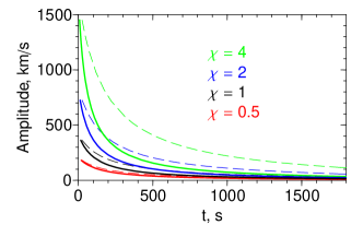
Figure 7.: The amplitude damping of shock waves (solid lines) and linear ones (dashed lines) calculated for the wave source energy $\tilde{\varepsilon}=10^{29}$ erg and different initial amplitudes. The initial amplitude values are specified in the figure as ratios $\chi$ of those to a fast-mode speed in the wave source.F-EUV˙decay

With respect to the damping of shock waves having the same initial lengths, amplitude decrease is faster for a wave with a higher amplitude. Therefore, shock waves with different initial amplitudes decay to the same level after approximately equal duration (Figure F-EUV_decay, solid curves). For comparison, we also plot the amplitude curves of linear disturbances, which hold an initial ratio of the wave amplitudes throughout propagation. The mentioned property of nonlinear waves (in Figure F-EUV_decay) allows us to be not precise about the value of the initial wave amplitude. Therefore, we can use the value that follows from the strong point-like explosion theory.

4 Discussion and Conclusion

S-conclusion

We have modeled the propagation of shock-associated EUV waves and Moreton waves, using the nonlinear geometrical acoustics method. This method takes into account characteristic properties of nonlinear waves: i) dependence of the wave velocity on its amplitude, ii) wave energy dissipation in the shock front, and iii) wave duration increase with time. The method allows one to calculate the nonlinear evolution of the shock wave and its propagation pattern. However, the generally accepted variant of this approach includes nonlinearity effects only for describing the amplitude and duration of a wave, but not for the wave velocity value. So, using such a non-self-consistent approach results in the loss of an important effect concerning wave kinematics.

We have applied another approach, appending an additional term to the ray equations. This has allowed the finite wave amplitude to be taken into account. We have solved self-consistently the modified ray equations and the equations describing the wave amplitude and duration evolution along a ray tube. It is this approach that has been developed in this paper to analyze coronal shock wave propagation along the solar surface.

One of the results of our analysis is the deceleration of EUV and Moreton waves at the initial stage of propagation. Since we use a spherically symmetric and isothermal model of the solar corona, deceleration is a direct consequence of their nonlinearity. Thus, EUV and Moreton waves having a sufficient amplitude (and therefore being observable) have to decelerate in the quiet Sun’s regions where average plasma parameters are constant along the solar surface. Note that the large-scale waves under study are registered just in these regions. Calculated wave deceleration is supported by the EUV and Moreton wave observations analyzed by Warmuth et al. (2001; 2004a). Also we notice here that EUV waves not associated with a coronal MHD wave show only slight or no deceleration (see, e.g., WillsDavey09).

The simple corona model also let us find other features of wave kinematics, e.g., i) the wave source height has effect on the initial portion of the velocity plot, and ii) the rate of wave deceleration and damping becomes lower as the wave source energy (or the wave length, respectively) grows. All these findings are applied for modeling EUV wave propagation in the 17 January 2010 event in an accompanying paper Grechnev et al. (2011a).

Modeling waves in the linear approximation does not reveal their deceleration. On the contrary, linear waves undergo only small acceleration caused by a slightly increasing inclination of the coronal wave front over the solar surface. This effect was first discovered by Uchida68. However, because of the error that he made in the expression for the barometric distribution of the coronal plasma density (the scale height was halved), the wave front inclination over the solar surface was very large. As a result, linear waves underwent considerable acceleration in Uchida’s original model.

Another important result of our modeling is the duration (and length) increase of Moreton and EUV waves. This effect is also confirmed by observations (see, e.g., Warmuth01; Veronig10). In contrast, a linear disturbance keeps its duration unchanged in a steady-state medium. Note that in the linear approximation, the wave amplitude and duration also vary due to the viscosity, the thermal conductivity and the finite plasma conductivity, however, these effects are negligible against nonlinear factors.

To summarize, we believe that wave deceleration and its duration increase, both being the attributes of shock wave evolution, point out the crucial role of nonlinearity in the behavior of EUV and Moreton waves (at least, it concerns some of them).

In conclusion, we will briefly discuss the method limitations for solving the shock wave propagation problem. The main limitation is associated with laws (E-damping_laws) of a shock wave damping, which are derived by using the relations for simple flat MHD waves in a homogeneous medium. So, we have to meet two requirements. First, the shock wave length should be smaller than the radius of curvature of the wave front and the smallest medium variation scale. The fulfilment of these conditions also ensures validity of the linear ray approximation (E-ray_eq_system), which involves actually even less limitations. The smallest variation scale in our modeling is that of plasma density. So, we are aware that our computation lies at the boundary of applicability of nonlinear geometrical acoustics since characteristic shock wave length $\Lambda$ and density scale $\rho/\left|\nabla\rho\right|$ are of the same order of magnitude.

Second, the nonlinear factor $U_{sh}/a$ should be small. Under this condition, damping laws (E-damping_laws) are derived and this very condition ensures a correct calculation of the terms involving $U_{sh}$ in the ray equations system (E-nonlin_ray_eq_system). With respect to the limitations of laws (E-damping_laws), the point-like atmospheric explosion theory Kestenboim, Roslyakov, and Chudov (1974) suggests that these laws describe satisfactorily spherical shock wave propagation up to $U_{sh}/a\leq 1$. When we choose the initial value $U_{sh}=a$ in Section S-modeling, we do not therefore go beyond the scope of the application of relations (E-damping_laws). However, ray equations (E-nonlin_ray_eq_system) and equations (E-eq_system_for_calc amp) at $U_{sh}/a\approx 1$ are able to yield an error in calculations. Nevertheless, this error is insignificant due to the nearly spherical shape of the wave front at the initial phase of propagation and then it disappears owing to rapid decrease in $U_{sh}$.

Acknowledgements

We thank Dr. V.V. Grechnev for useful discussions and valuable help in preparing the paper. We also thank the anonymous referee and editors for careful reading of the manuscript as well as helpful comments and suggestions. A.A. is very grateful to the scientific organizing committee of the CESRA2010 Workshop for financial support.

The research was supported by the Russian Foundation of Basic Research (Grant No. 10–02–09366) and Siberian Branch of the Russian Academy of Sciences (Lavrentyev Grant 2010–2011).

References

- Balasubramaniam, Pevtsov, and Neidig (2007) Balasubramaniam, K. S., Pevtsov, A. A., Neidig, D. F.: 2007, ApJ 658, 1372.
- Barnes (1992) Barnes, A.: 1992, J. Geophys. Res. 97, 12105.
- Blokhintsev (1981) Blokhintsev, D. I.: 1981, Acoustics of an Inhomogeneous Moving Medium, 2nd edn., Nauka, Moscow (in Russian).
- Gilbert et al. (2004) Gilbert, H. R., Holzer, T. E., Thompson, B. J., Burkepile, J. T.: 2004, ApJ 607, 540.
- Grechnev et al. (2011a) Grechnev, V. V., Afanasyev, A. N., Uralov, A. M., Chertok, I. M., Eselevich, M. V., Eselevich, V. G., Rudenko, G. V., Kubo, Y.: 2011a, Sol. Phys. in this issue.
- Grechnev et al. (2011b) Grechnev, V. V., Uralov, A. M., Chertok, I. M., Kuzmenko, I. V., Afanasyev, A. N., Meshalkina, N. S., Kalashnikov, S. S., Kubo, Y.: 2011b, Sol. Phys. in this issue.
- Hudson et al. (2003) Hudson, H.S., Khan, J.I., Lemen, J.R., Nitta, N.V., Uchida, Y.: 2003, Sol. Phys. 212, 121.
- Kestenboim, Roslyakov, and Chudov (1974) Kestenboim, Kh. S., Roslyakov, G. S., Chudov, L. A.: 1974, The Point Explosion, Nauka, Moscow (in Russian).
- Khan and Aurass (2002) Khan, J. I., Aurass, H.: 2002, A&A 383, 1018.
- Kravtsov and Orlov (1990) Kravtsov, Y. A., Orlov, Y. I.: 1990, Geometrical Optics of Inhomogeneous Media, Springer-Verlag, Berlin.
- Kulikovsky and Lyubimov (2005) Kulikovsky, A. G., Lyubimov, G. A.: 2005, Magnetic Hydrodynamics, 2nd edn., Logos, Moscow (in Russian).
- Landau and Lifshitz (1987) Landau, L. D., Lifshitz, E. M.: 1987, Fluid Mechanics, 2nd edn., Pergamon Press, Oxford.
- Mann et al. (2003) Mann, G., Klassen, A., Aurass, H., Classen, H.-T.: 2003, A&A 400, 329.
- Mann et al. (1999) Mann, G., Jansen, F., MacDowall, R.J., Kaiser, M.L., Stone, R.G.: 1999, A&A 348, 614.
- Moreton and Ramsey (1960) Moreton, G. E., Ramsey, H. E.: 1960, PASJ 72, 357.
- Muhr et al. (2010) Muhr, N., Vršnak, B., Temmer, M., Veronig, A.M., Magdalenić, J.: 2010, ApJ 708, 1639.
- Narukage et al. (2004) Narukage, N., Eto, S., Kadota, M., Kitai, R., Kurokawa, H., Shibata, K.: 2004, in A.V. Stepanov, E.E. Benevolenskaya, A.G. Kosovichev (eds.), Multi-Wavelength Investigations of Solar Activity, Proc. IAU Symp. 223, 367.
- Narukage et al. (2002) Narukage, N., Hudson, H.S., Morimoto, T., Akiyama, S., Kitai, R., Kurokawa, H., Shibata, K.: 2002, ApJ 572, L109.
- Patsourakos et al. (2009) Patsourakos, S., Vourlidas, A., Wang, Y. M., Stenborg, G., Thernisien, A.: 2009, Sol. Phys. 259, 49.
- Temmer et al. (2009) Temmer, M., Vršnak, B., Žic, T., Veronig, A. M.: 2009, ApJ 702, 1343.
- Uchida (1960) Uchida, Y.: 1960, PASJ 12, 376.
- Uchida (1968) Uchida, Y.: 1968, Sol. Phys. 4, 30.
- Uchida (1974) Uchida, Y.: 1974, Sol. Phys. 39, 431.
- Uchida, Altschuler, and Newkirk (1973) Uchida, Y., Altschuler, M. D., Newkirk, G., Jr.: 1973, Sol. Phys. 28, 495.
- Uralov (1982) Uralov, A. M.: 1982, Magnitnaya Gidrodinamika No. 1, 45 (in Russian).
- Uralova and Uralov (1994) Uralova, S. V., Uralov, A. M.: 1994, Sol. Phys. 152, 457.
- Veronig et al. (2010) Veronig, A. M., Muhr, N., Kienreich, I. W., Temmer, M., Vršnak, B.: 2010, ApJ 716, L57.
- Vršnak and Lulić (2000) Vršnak, B., Lulić, S.: 2000, Sol. Phys. 196, 157.
- Vršnak et al. (2002a) Vršnak, B., Magdalenić, J., Aurass, H., Mann, G.: 2002a, A&A 396, 673.
- Vršnak et al. (2002b) Vršnak, B., Warmuth, A., Brajša, R., Hanslmeier, A.: 2002b, A&A 394, 299.
- Vršnak et al. (2005) Vršnak, B., Magdalenić, J., Temmer, M., Veronig, A., Warmuth, A., Mann, G., Aurass, H., Otruba, W.: 2005, ApJ 625, L67.
- Wang (2000) Wang, Y.-M.: 2000, ApJ 543, L89.
- Warmuth, Mann, and Aurass (2005) Warmuth, A., Mann, G., Aurass, H.: 2005, ApJ 626, L121.
- Warmuth et al. (2001) Warmuth, A., Vršnak, B., Aurass, H., Hanslmeier, A.: 2001, ApJ 560, L105.
- Warmuth et al. (2004a) Warmuth, A., Vršnak, B., Magdalenić, J., Hanslmeier, A., Otruba, W.: 2004a, A&A 418, 1101.
- Warmuth et al. (2004b) Warmuth, A., Vršnak, B., Magdalenić, J., Hanslmeier, A., Otruba, W.: 2004b, A&A 418, 1117.
- White and Thompson (2005) White, S. M., Thompson, B. J.: 2005, ApJ 620, L63.
- Wills-Davey and Attrill (2009) Wills-Davey, M. J., Attrill, G. D. R.: 2009, Space Sci. Rev. 149, 325.
- Žic et al. (2008) Žic, T., Vršnak, B., Temmer, M., Jacobs, C.: 2008, Sol. Phys. 253, 237.