Distance Transform Gradient Density Estimation using the Stationary Phase Approximation

Abstract

The complex wave representation (CWR) converts unsigned 2D distance transforms into their corresponding wave functions. Here, the distance transform $S(X)$ appears as the phase of the wave function $\phi(X)$—specifically, $\phi(X)=\exp\left(\frac{iS(X)}{\tau}\right)$ where $\tau$ is a free parameter. In this work, we prove a novel result using the higher-order stationary phase approximation: we show convergence of the normalized power spectrum (squared magnitude of the Fourier transform) of the wave function to the density function of the distance transform gradients as the free parameter $\tau\rightarrow 0$. In colloquial terms, spatial frequencies are gradient histogram bins. Since distance transform gradients carry only orientation information (as their magnitudes are identically equal to one almost everywhere), the 2D Fourier transform values mainly lie on the unit circle in the spatial frequency domain as $\tau\rightarrow 0$. The proof of the result involves standard integration techniques and requires proper ordering of limits. Our mathematical relation indicates that the CWR of distance transforms is an intriguing, new representation.

1 Introduction

Euclidean distance functions (more popularly referred to as distance transforms) are widely used in many domains [17, 22]. An important subset—point-set based distance functions—also finds application in many domains with computer vision being a prominent example [22, 11, 20]. Since distance transforms allow us to transition from shapes to a scalar field, problems such as shape registration are often couched in terms of rigid, affine or nonrigid alignment of distance transform fields, where the shapes are parameterized as a set of points [19]. In medical imaging, they are used in the construction of neuroanatomical shape complex atlases based on an information geometry framework [2].

Even when one begins with a set of closed curves (as a shape template for example), the curves are often discretized to yield a point-set prior to the application of fast sweeping [25] and other distance transform estimation methods. Signed and unsigned distance transforms are deployed in 3D as well with their zero level-sets corresponding to surfaces. Furthermore, medial axis methods and skeletonization often involve distance transform representations [13]. In the domain of computer vision, the gradient density function is popularly known as the histogram of oriented gradients (HOG). Since the advent of HOG a few years ago, gradient density estimation has risen in prominence and is employed in human recognition systems [4].

The distance transform for a set of $K$ discrete points $Y=\{Y_{k}\in\mathbb{R}^{D}\},k\in\{1,\ldots,K\}$ where $D$ is the dimensionality of the point-set is defined as

$$S(X)\equiv\min_{k}\|X-Y_{k}\|,$$ (1)

where $X\in\Omega$ is a closed bounded domain in $\mathbb{R}^{D}$. In this article, we are only concerned with $D=2$.

In computational geometry, Euclidean distance functions correspond to the Voronoi problem [5] and the solution $S(X)$ can be visualized as a set of cones (with the centers being the point-set locations $\{Y_{k}\}$). The distance transform satisfies the static, non-linear Hamilton-Jacobi equation

$$\|\nabla S\|=1$$ (2)

almost everywhere, barring the point-set locations and the Voronoi boundaries where it is not differentiable [17, 18, 21]. Here $\nabla S=(S_{x},S_{y})$ denotes the gradients of $S$ and $\|\cdot\|$ represents its Euclidean magnitude. Furthermore $S(X)=0$ at the point-set locations. Following the wave optics literature, one can envisage light waves simultaneously emanating from the given point sources and propagating with a velocity of one in all directions. The value of $S$ at a grid point $X_{0}$, namely $S(X_{0})$, corresponds to the time taken by the first light wave (out of the $K$ light waves) to reach the grid location $X_{0}$. Driven by this optics analogy, when we express $S$ as the phase of a wave function $\phi$ as in

$$\phi=\exp\left(\frac{iS}{\tau}\right),$$ (3)

we made an intriguing empirical observation. The power spectrum of the wave function approximates the density function of the gradients of the distance transform as the parameter $\tau$ in Equation 3 tends to zero. In this paper, we formally prove this result. We refer to this wave function $\phi$ which satisfies the phase relation with $S$ as the Complex Wave Representation (CWR) of distance transforms.

2 Main Contribution

The centerpiece of this work is to provide a useful application of the stationary phase method, wherein we show an equivalence between the density function of the gradients of the distance function $\nabla S=(S_{x},S_{y})$ and the power spectrum (squared magnitude of the Fourier transform) of the CWR ($\phi$) as the free parameter $\tau$ (in Equation 3) approaches zero. Here, the density function of the gradients is obtained via a random variable transformation of a uniformly distributed random variable $W$ (over the bounded domain $\Omega$) using the gradients $\nabla S=(S_{x},S_{y})$ as the transformation functions. In other words, if we define a random variable $Z=\nabla S(W)$ where the random variable $W$ has a uniform distribution on a closed bounded domain $\Omega\subset\mathbb{R}^{2}$, the density function of $Z$ represents the density function of the gradients of the distance transform.

As the norm of the gradients $\nabla S$ is defined to be $1$ almost everywhere (from Equation 2), we observe that the density function of the gradients is one-dimensional and defined over the space of orientations. Section 3 provides a closed-form expression for this density function. As the gradients are unit vectors, we notice that the Fourier transform values of the CWR ($\phi$) lie mainly on the unit circle and this behavior tightens as $\tau\rightarrow 0$. Specifically, if $F_{\tau}(\tilde{r},\omega)$ represents the Fourier transform of $\phi$ in the polar coordinate system at a given value of $\tau$, Theorem 2 demonstrates that if $\tilde{r}\not=1$, then $\lim_{\tau\rightarrow 0}F_{\tau}(\tilde{r},\omega)=0$.

Our main result is established in Theorem 4 where we show that the power spectrum of the wave function $\phi$ when polled close to the unit circle, is approximately equal to the density function of the distance transform gradients, with the approximation becoming increasingly exact as $\tau\rightarrow 0$. In other words, if $P(\omega)$ denotes the closed-form density of the gradients defined over the orientation $\omega$ and if $P_{\tau}(\tilde{r},\omega)$ corresponds to the power spectrum of $\phi$ represented in the polar coordinate system at a given value of $\tau$, Theorem 4 constitutes the following relation

$$\lim_{\delta\rightarrow 0}\lim_{\tau\rightarrow 0}\int_{\omega_{0}}^{\omega_{0}+\Delta}\left\{\int_{1-\delta}^{1+\delta}P_{\tau}(\tilde{r},\omega)\tilde{r}d\tilde{r}\right\}d\omega=\int_{\omega_{0}}^{\omega_{0}+\Delta}P(\omega)d\omega$$ (4)

for any (small) value of the interval measure $\Delta$ on $\omega$. We show this result using the higher-order stationary phase approximation, a well known technique in asymptotic analysis [23]. Through the pioneering works of Jones and Kline [12], Olver [15], Wong [23], McClure and Wong [14], among others, the stationary phase approximation has become a widely deployed tool in the approximation of oscillatory integrals. Our work showcases a novel application of the stationary phase method for estimating the probability density function of distance transform gradients. The significance of our mathematical result is that spatial frequencies become histogram bins and hence the power spectrum $P_{\tau}$ can serve as a gradient density estimator at small, non-zero values of $\tau$. We would like to emphasize that our work is fundamentally different from estimating the gradients of a density function [8] and should not be semantically confused with it.

2.1 Motivation from quantum mechanics

Our new mathematical relationship is motivated by the classical-quantum relation, wherein classical physics is expressed as a limiting case of quantum mechanics [10, 6]. When $S$ is treated as the Hamilton-Jacobi scalar field, the gradients of $S$ correspond to the classical momentum of a particle [9]. In the parlance of quantum mechanics, the squared magnitude of the wave function expressed either in its position or momentum basis corresponds to its position or momentum density respectively. Since these representations (either in the position or momentum basis) are simply (suitably scaled) Fourier transforms of each other, the squared magnitude of the Fourier transform of the wave function expressed in its position basis is its quantum momentum density. However, the time independent Schrödinger wave function $\phi(x,y)$ (expressed in its position basis) can be approximated by $\exp\left(\frac{iS(x,y)}{\tau}\right)$ as $\tau\rightarrow 0$ [6]. Here $\tau$ (treated as a free parameter in our work) represents Planck’s constant. Hence the squared magnitude of the Fourier transform $\exp\left(\frac{iS(x,y)}{\tau}\right)$ corresponds to the quantum momentum density of $S$. The principal results proved in the article (Theorem 4 and Proposition 12) state that the classical momentum density (denoted by $P$) can be expressed as a limiting case (as $\tau\rightarrow 0$) of its corresponding quantum momentum density (denoted by $P_{\tau}$), in agreement with the correspondence principle.

3 The Distance Transform Gradient Density Function

As mentioned above, the geometry of the distance transform corresponds to a set of intersecting cones with the origins at the Voronoi centers [5]. The gradients of the distance transform (which exist globally except at the cone intersections and origins) are unit vectors and satisfy Equation 2. Therefore the gradient density function is one-dimensional and defined over the space of orientations. The orientations are constant and unique along each ray of each cone. Its probability distribution function is given by

$$\mathcal{F}(\theta\leq\Theta\leq\theta+\Delta)\equiv\frac{1}{L}\int\int_{\theta\leq\arctan\left(\frac{S_{y}}{S_{x}}\right)\leq\theta+\Delta}dxdy$$ (5)

where $L$ is the area of the bounded domain $\Omega$. We have expressed the orientation random variable as $\Theta=\arctan\left(\frac{S_{y}}{S_{x}}\right)$. The probability distribution function also induces a closed-form expression for its density function as shown below.

Let $\Omega\subset\mathbb{R}^{2}$ denote a polygonal grid such that its boundary $\partial\Omega$ is composed of a finite sequence of straight line segments. The reason for restricting only to polygonal domains with boundaries made of line segments will become clear when we discuss Theorem 2. Let the set $Y=\{Y_{k}\in\mathbb{R}^{2},k\in\{1,\ldots,K\}\}$ be the given point-set locations and let $Y_{k}=(x_{k},y_{k})$. Then the Euclidean distance transform at a point $X=(x,y)\in\Omega$ is given by

$$S(X)\equiv\min_{k}\|X-Y_{k}\|=\min_{k}(\sqrt{(x-x_{k})^{2}+(y-y_{k})^{2}}).$$ (6)

Let $\mathcal{D}_{k}$, centered at $Y_{k}$, denote the $k^{th}$ Voronoi region corresponding to the input point $Y_{k}$. $\mathcal{D}_{k}$ can be represented by a Cartesian product $[0,2\pi)\times[0,R_{k}(\theta)]$ where $R_{k}(\theta)$ is the length of the ray of the $k^{th}$ cone at an orientation $\theta$. If a grid point $X=(x,y)\in\left(Y_{k}+\mathcal{D}_{k}\right)$, then $S(X)=\|X-Y_{k}\|$. Each $\mathcal{D}_{k}$ is a convex polygon whose boundary $\partial\mathcal{D}_{k}$ is also composed of a finite sequence of straight line segments as shown in Figure 1.

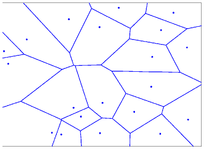
Figure 1: Voronoi diagram of the given $K$ points. Each Voronoi boundary is composed of straight line segments.

Note that even for points that lie on the Voronoi boundary where the radial length equals $R_{k}(\theta)$, the distance transform is well defined. The area $L$ of the polygonal grid $\Omega$ is given by

$$L\equiv\sum_{k=1}^{K}\int_{0}^{2\pi}\int_{0}^{R_{k}(\theta)}rdrd\theta=\sum_{k=1}^{K}\int_{0}^{2\pi}\frac{R_{k}^{2}(\theta)}{2}d\theta.$$ (7)

With the above set-up in place, after recognizing the cone geometry at each Voronoi center $Y_{k}$, Equation 5 can be simplified as

$$\mathcal{F}(\theta\leq\Theta\leq\theta+\Delta)\equiv\frac{1}{L}\sum_{k=1}^{K}\int_{\theta}^{\theta+\Delta}\int_{0}^{R_{k}(\theta)}rdrd\theta=\frac{1}{L}\sum_{k=1}^{K}\int_{\theta}^{\theta+\Delta}\frac{R_{k}^{2}(\theta)}{2}d\theta.$$ (8)

Following this drastic simplification, we can write the closed-form expression for the density function of the unit vector distance transform gradients as

$$P(\theta)\equiv\lim_{\Delta\rightarrow 0}\frac{\mathcal{F}(\theta\leq\Theta\leq\theta+\Delta)}{\Delta}=\frac{1}{L}\sum_{k=1}^{K}\frac{R_{k}^{2}(\theta)}{2}.$$ (9)

Based on the expression for $L$ in Equation 7, it is easy to see that

$$\int_{0}^{2\pi}P(\theta)d\theta=1.$$ (10)

Since the Voronoi cells are convex polygons [5], each cell contributes exactly one conical ray to the density function on orientation.

4 Properties of the Fourier Transform of the CWR

Since the distance transform is not differentiable at the point-set locations $\{Y_{k}\}_{k=1}^{K}$ and also along the Voronoi boundaries $\partial\mathcal{D}_{k},\forall k$ (a measure zero set in 2D), we restrict ourselves to the region which excludes both of them. To this end, let $0<\epsilon<\frac{1}{2}$ be given. Let the region $\mathcal{D}_{k}^{\epsilon}$ centered at $Y_{k}$ be represented by the Cartesian product $[0,2\pi)\times[R_{k}^{(1)}(\theta),R_{k}^{(2)}(\theta)]$ where,

$$R_{k}^{(1)}(\theta) = \epsilon R_{k}(\theta)\hskip 10.0pt\mbox{and}$$

$$R_{k}^{(2)}(\theta) = (1-\epsilon)R_{k}(\theta).$$ (11)

The length of the ray at the orientation $\theta$ in $\mathcal{D}_{k}^{\epsilon}$ equals $R_{k}^{(2)}(\theta)-R_{k}^{(1)}(\theta)$. Note that in the definition of $\mathcal{D}_{k}^{\epsilon}$, we have explicitly removed the source point $Y_{k}$ where the ray length $r(\theta)=0$ and the boundary of the Voronoi cell where $r(\theta)=R_{k}(\theta)$ as shown in Figure 2.

Figure 2: Region that excludes both the source point and the Voronoi boundary.

Define the grid

$$\Omega^{\epsilon}\equiv\bigcup_{k=1}^{K}\left(Y_{k}+\mathcal{D}_{k}^{\epsilon}\right).$$ (12)

Its area $L^{\epsilon}$ equals

$$L^{\epsilon}\equiv\sum_{k=1}^{K}\int_{0}^{2\pi}\int_{R_{k}^{(1)}(\theta)}^{R_{k}^{(2)}(\theta)}rdrd\theta=(1-2\epsilon)\sum_{k=1}^{K}\int_{0}^{2\pi}\frac{R_{k}^{2}(\theta)}{2}d\theta.$$ (13)

From Equation 7 we get $L^{\epsilon}=(1-2\epsilon)L$ and hence $\lim_{\epsilon\rightarrow 0}L^{\epsilon}=L$.

Let $l^{\epsilon}=\sqrt{L^{\epsilon}}$. Define a function $F^{\epsilon}:\mathbb{R}\times\mathbb{R}\times\mathbb{R}\rightarrow\mathbb{C}$ as

$$F^{\epsilon}(u,v,\tau)\equiv\frac{1}{2\pi\tau l^{\epsilon}}\iint\limits_{\Omega^{\epsilon}}\exp\left(\frac{iS(x,y)}{\tau}\right)\exp\left(\frac{-i(ux+vy)}{\tau}\right)dxdy.$$ (14)

For a fixed value of $\tau$, define a function $F_{\tau}^{\epsilon}:\mathbb{R}\times\mathbb{R}\rightarrow\mathbb{C}$ as

$$F_{\tau}^{\epsilon}(u,v)\equiv F^{\epsilon}(u,v,\tau).$$ (15)

Note that $F_{\tau}^{\epsilon}$ is closely related to the Fourier transform of the CWR, $\phi=\exp\left(\frac{iS}{\tau}\right)$ [1]. The scale factor $\frac{1}{2\pi\tau l^{\epsilon}}$ is the normalization factor such that the $\ell_{2}$ norm of $F_{\tau}^{\epsilon}$ is 1 as seen in the following Lemma (with the proof given in Appendix A).

Lemma 1.

With $F_{\tau}^{\epsilon}$ defined as above, $F_{\tau}^{\epsilon}\in L^{2}(\mathbb{R}^{2})$ and $\|F_{\tau}^{\epsilon}\|=1$.

Consider the polar representation of the spatial frequencies $(u,v)$ namely $u=\tilde{r}\cos(\omega)$ and $v=\tilde{r}\sin(\omega)$ where $\tilde{r}>0$. For $(x,y)\in\left(Y_{k}+\mathcal{D}_{k}^{\epsilon}\right)$, let $x-x_{k}=r\cos(\theta)$ and $y-y_{k}=r\sin(\theta)$ where $r\in[R_{k}^{(1)}(\theta),R_{k}^{(2)}(\theta)]$. Then Equation 14 can be rewritten as

$$F_{\tau}^{\epsilon}(\tilde{r},\omega)=\sum_{k=1}^{K}C_{k}I_{k}(\tilde{r},\omega)$$ (16)

where

$$C_{k}=\exp\left\{-\frac{i}{\tau}\left[\tilde{r}\cos(\omega)x_{k}+\tilde{r}\sin(\omega)y_{k}\right]\right\}$$ (17)

and

$$I_{k}(\tilde{r},\omega)=\frac{1}{2\pi\tau l^{\epsilon}}\int_{0}^{2\pi}\int_{R_{k}^{(1)}(\theta)}^{R_{k}^{(2)}(\theta)}\exp\left\{\frac{i}{\tau}r\left[1-\tilde{r}\cos(\theta-\omega)\right]\right\}rdrd\theta.$$ (18)

With the above set-up in place, we have the following theorem, namely,

Theorem 2.

[Circle Theorem] If $\tilde{r}\not=1$, then,

$$\lim_{\tau\rightarrow 0}F_{\tau}^{\epsilon}(\tilde{r},\omega)=0,$$ (19)

for any $0<\epsilon<\frac{1}{2}$.

4.1 An Intuitive Examination of Theorem 2

Before we furnish a rigorous proof for the aforementioned theorem, we provide an intuitive picture of why the statement is true. Observe that the first exponential $\exp\left(\frac{iS(x,y)}{\tau}\right)$ in Equation 14 is a varying complex "sinusoid" and the second exponential $\exp\left(\frac{-i(ux+vy)}{\tau}\right)$ in Equation 14 is a fixed complex sinusoid at frequencies $\frac{u}{\tau}$ and $\frac{v}{\tau}$ along the $x$- and $y$-coordinate axes respectively. When we multiply these two complex exponentials, at low values of $\tau$, the two sinusoids are usually not "in sync" and cancellations occur in the integral. Exceptions to the cancellation happen at locations where $\nabla S=(S_{x},S_{y})=(u,v)$, as around these locations, the two sinusoids are in perfect sync. Since $\|\nabla S\|=1$ for distance transforms, strong resonance occurs only when $u^{2}+v^{2}=1$ ($\tilde{r}=1$). When $\tilde{r}\not=1$, the two sinusoids tend to cancel each other out as $\tau\rightarrow 0$, resulting in $F_{\tau}^{\epsilon}$ becoming zero at these locations.

4.2 Proof of Theorem 2

Having given an intuitive picture of why Theorem 2 holds true, we now proceed with the formal proof. As each $C_{k}$ is bounded, it suffices to show that if $\tilde{r}\not=1$, then $\lim_{\tau\rightarrow 0}I_{k}(\tilde{r},\omega)=0$ for all $I_{k}$.

Proof.

Consider the integral

$$I(\tilde{r},\omega)=\frac{1}{2\pi\tau l^{\epsilon}}\int_{0}^{2\pi}\int_{R^{(1)}(\theta)}^{R^{(2)}(\theta)}\exp\left\{\frac{i}{\tau}r\left[1-\tilde{r}\cos(\theta-\omega)\right]\right\}rdrd\theta,$$ (20)

where $R^{(1)}(\theta)=\epsilon R(\theta)$ and $R^{(2)}(\theta)=(1-\epsilon)R(\theta)$. Let the region $[0,2\pi)\times[R^{(1)}(\theta),R^{(2)}(\theta)]$ be denoted by $\mathcal{D}^{\epsilon}$. $R(\theta)$ is defined in such a way that the boundary of $D^{\epsilon}$ consists of a finite sequence of straight line segments as in the case of each $\mathcal{D}_{k}^{\epsilon}$. Notice that $\mathcal{D}^{\epsilon}$ doesn’t contain the origin $(0,0)$. In order to prove Theorem 2, it is sufficient to show that $\lim_{\tau\rightarrow 0}I(\tilde{r},\omega)=0$.

Let $p(r,\theta;\tilde{r},\omega)=r(1-\tilde{r}\cos(\theta-\omega))$ denote the phase term of $I$ in Equation 20 for a given $\tilde{r}$ and $\omega$. The partial derivatives of $p(r,\theta;\tilde{r},\omega)$ (with $\tilde{r}$ and $\omega$ held fixed) are given by

$$\frac{\partial p}{\partial r}=1-\tilde{r}\cos(\theta-\omega),\hskip 10.0pt\frac{\partial p}{\partial\theta}=r\tilde{r}\sin(\theta-\omega).$$ (21)

Since $\mathcal{D}^{\epsilon}$ is bounded away from the origin $(0,0)$, $\nabla p$ is well-defined and bounded and equals zero only when $\tilde{r}=1$ and $\theta=\omega$. Since $\tilde{r}\not=1$ by assumption, no stationary point exists ($\nabla p\not=0$) and hence we can expect $I(\tilde{r},\omega)\rightarrow 0$ as $\tau\rightarrow 0$ [3, 12, 24]. Below, we show this result more explicitly.

Define a vector field $\mathbf{u}(r,\theta;\tilde{r},\omega)=\frac{\nabla p}{\|\nabla p\|^{2}}r$ at a fixed value of $\tilde{r}$ and $\omega$. Note that

$$\nabla\cdot\left[\mathbf{u}(r,\theta;\tilde{r},\omega)\exp\left(\frac{ip(r,\theta;\tilde{r},\omega)}{\tau}\right)\right] = \left(\nabla\cdot\mathbf{u}(r,\theta;\tilde{r},\omega)\right)\exp\left(\frac{ip(r,\theta;\tilde{r},\omega)}{\tau}\right)$$ (22)

$$+ \frac{i}{\tau}\exp\left(\frac{ip(r,\theta;\tilde{r},\omega)}{\tau}\right)r$$

where the gradient operator $\nabla=\left(\frac{\partial}{\partial r},\frac{1}{r}\frac{\partial}{\partial\theta}\right)$. Inserting Equation 22 in Equation 20, we get

$$I(\tilde{r},\omega)=I^{(1)}(\tilde{r},\omega)-I^{(2)}(\tilde{r},\omega),$$ (23)

where

$$I^{(1)}(\tilde{r},\omega) = \frac{1}{2\pi il^{\epsilon}}\iint\limits_{\mathcal{D}^{\epsilon}}\nabla\cdot\left(\mathbf{u}(r,\theta;\tilde{r},\omega)\exp\left(\frac{ip(r,\theta;\tilde{r},\omega)}{\tau}\right)\right)drd\theta,\,\mathrm{and}$$

$$I^{(2)}(\tilde{r},\omega) = \frac{1}{2\pi il^{\epsilon}}\iint\limits_{\mathcal{D}^{\epsilon}}\left(\nabla\cdot\mathbf{u}(r,\theta;\tilde{r},\omega)\right)\exp\left(\frac{ip(r,\theta;\tilde{r},\omega)}{\tau}\right)drd\theta.$$ (24)

Consider the integral $I^{(1)}(\tilde{r},\omega)$. From the divergence theorem, we have

$$I^{(1)}(\tilde{r},\omega)=\frac{1}{2\pi il^{\epsilon}}\int_{\Gamma}(\mathbf{u}^{T}\mathbf{n})\exp\left(\frac{ip(r,\theta;\tilde{r},\omega)}{\tau}\right)ds$$ (25)

where $\Gamma$ is the positively oriented boundary of $\mathcal{D}^{\epsilon}$, $s$ is the arc length of $\Gamma$ and $\mathbf{n}$ is the unit outward normal of $\Gamma$. The boundary $\Gamma$ consists of two disjoint regions, one along $r(\theta)=R^{(1)}(\theta)$ and another along $r(\theta)=R^{(2)}(\theta)$. If the level curves of $p(r,\theta;\tilde{r},\omega)$ are tangential to $\Gamma$ only at a discrete set of locations giving rise to stationary points of the second kind [23, 24, 14]—in other words, if $p(r,\theta;\tilde{r},\omega)$ is not constant along the boundary $\Gamma$ for any contiguous interval of $\theta$—then, using the one dimensional stationary phase approximation [15, 16], $I^{(1)}(\tilde{r},\omega)$ can be shown to be $O(\sqrt{\tau})$ and hence converges to zero as $\tau\rightarrow 0$. Since the boundary of $\mathcal{D}^{\epsilon}$ is composed of straight line segments (specifically not arc-like), we can show that the level curves of $p(r,\theta;\tilde{r},\omega)$ cannot overlap with $\Gamma$ for a non-zero finite interval. (The next paragraph takes care of this technical issue and can be skipped without loss of continuity.)

The level curves of $p(r,\theta;\tilde{r},\omega)$ are given by $R(\theta)(1-\tilde{r}\cos(\theta-\omega))=c$, where $c$ is a constant. Recall that each of the two disjoint regions of $\Gamma$ is composed of a finite sequence of line segments. For the level curves of $p(r,\theta;\tilde{r},\omega)$ to coincide with $\Gamma$ over a non-zero finite interval, $y(\theta)=R(\theta)\sin(\theta)=\frac{c\sin(\theta)}{1-\tilde{r}\cos(\theta-\omega)}$ and $x(\theta)=R(\theta)\cos(\theta)=\frac{c\cos(\theta)}{1-\tilde{r}\cos(\theta-\omega)}$ should satisfy the line equation $y=mx+b$ for some slope $m$ and slope-intercept $b$, when $\theta$ varies over some contiguous interval $\theta\in[\theta_{1},\theta_{2}]$. Plugging in the value of $y(\theta)$ and $x(\theta)$ into the line equation and expanding $\cos(\theta-\omega)$, we have

$$c\sin\left(\theta\right)=mc\cos(\theta)+b-b\tilde{r}[\cos(\theta)\cos(\omega)+\sin(\theta)\sin(\omega)].$$ (26)

Combining the terms, we get

$$\sin(\theta)[c+b\tilde{r}\sin(\omega)]-\cos(\theta)[mc-b\tilde{r}\cos(\omega)]=b.$$ (27)

By defining $\lambda_{1}\equiv c+b\tilde{r}\sin(\omega)$ and $\lambda_{2}\equiv-(mc-b\tilde{r}\cos(\omega))$, we see that $\sin(\theta)$ and $\cos(\theta)$ need to satisfy the linear relation

$$\lambda_{1}\sin(\theta)+\lambda_{2}\cos(\theta)=b$$ (28)

for $\theta\in[\theta_{1},\theta_{2}]$ in order for the level curves of $p(r,\theta;\tilde{r},\omega)$ to overlap with the piece-wise linear boundary $\Gamma$. As Equation 28 cannot be true for a finite interval of $\theta$, $I^{(1)}(\tilde{r},\omega)=O(\sqrt{\tau})$ as $\tau\rightarrow 0$ and hence converges to zero in the limit.

Now $I^{(2)}(\tilde{r},\omega)$ has a similar form as the original $I(\tilde{r},\omega)$ in Equation 20 with $r$ replaced by $g_{1}(r,\theta;\tilde{r},\omega)=\left(\nabla\cdot\mathbf{u}\right)$. Letting $\mathbf{u}_{1}(r,\theta;\tilde{r},\omega)=\frac{\nabla p}{\|\nabla p\|^{2}}g_{1}(r,\theta;\tilde{r},\omega)$, from Equation 22 and the divergence theorem, we get

$$I^{(2)}(\tilde{r},\omega) = \frac{-\tau}{2\pi l^{\epsilon}}\int_{\Gamma}(\mathbf{u}_{1}^{T}\mathbf{n})\exp\left(\frac{ip(r,\theta;\tilde{r},\omega)}{\tau}\right)ds$$ (29)

$$+ \frac{\tau}{2\pi l^{\epsilon}}\iint\limits_{\mathcal{D}^{\epsilon}}\left(\nabla\cdot\mathbf{u}_{1}(r,\theta;\tilde{r},\omega)\right)\exp\left(\frac{ip(r,\theta;\tilde{r},\omega)}{\tau}\right)drd\theta.$$

As $I^{(2)}(\tilde{r},\omega)=O(\tau)$, it converges to zero as $\tau\rightarrow 0$. Applying the obtained results to Equation 23, we see that $I(\tilde{r},\omega)$ (and also $I_{k}(\tilde{r},\omega)$ defined in Equation 18) $\rightarrow 0$ as $\tau\rightarrow 0$ which completes the proof.

∎

Since Theorem 2 is true for any $0<\epsilon<\frac{1}{2}$, it also holds as $\epsilon\rightarrow 0$. As a corollary, we have the following result:

Corollary 3.

If $\tilde{r}\not=1$, then

$$\lim_{\epsilon\rightarrow 0}\lim_{\tau\rightarrow 0}F_{\tau}^{\epsilon}(\tilde{r},\omega)=0.$$ (30)

5 Spatial Frequencies as Gradient Histogram Bins

We now show that the squared magnitude of the Fourier transform of the CWR ($\phi$) when polled close to the unit circle ($\tilde{r}=1$) is approximately equal to the density function of the distance transform gradients ($P$) with the approximation becoming increasingly tight as $\tau\rightarrow 0$.

The squared magnitude of the Fourier transform—also called its power spectrum [1]—is given by

$$P_{\tau}^{\epsilon}(\tilde{r},\omega)\equiv|F_{\tau}^{\epsilon}(\tilde{r},\omega)|^{2}=F_{\tau}^{\epsilon}(\tilde{r},\omega)\overline{F_{\tau}^{\epsilon}(\tilde{r},\omega)}.$$ (31)

By definition, $P_{\tau}^{\epsilon}(\tilde{r},\omega)\geq 0$. From Lemma 1, we have

$$\int_{0}^{2\pi}\int_{0}^{\infty}P_{\tau}^{\epsilon}(\tilde{r},\omega)\tilde{r}d\tilde{r}d\omega=1$$ (32)

independent of $\tau$. Hence, $P_{\tau}^{\epsilon}(\tilde{r},\omega)$ can be treated as a density function for all values of $\tau$. We earlier observed that the gradient density function of the unit vector distance transform gradients is one-dimensional and defined over the space of orientations $\omega$. For $P_{\tau}^{\epsilon}(\tilde{r},\omega)$ to behave as an orientation density function, it needs to be integrated along the radial direction $\tilde{r}$. Since Theorem 2 states that the Fourier transform values are concentrated only on the unit circle $\tilde{r}=1$ and converges to zero elsewhere as $\tau\rightarrow 0$, it should be sufficient if the integration for $\tilde{r}$ is done over a region very close to $\tilde{r}=1$. The following theorem—the principal result in this paper—confirms our observation.

Theorem 4.

For any given $0<\epsilon<\frac{1}{2}$, $0<\delta<1$, $\omega_{0}\in[0,2\pi)$ and $0<\Delta<2\pi$,

$$\lim_{\tau\rightarrow 0}\int_{\omega_{0}}^{\omega_{0}+\Delta}\int_{1-\delta}^{1+\delta}P_{\tau}^{\epsilon}(\tilde{r},\omega)\tilde{r}d\tilde{r}d\omega=\int_{\omega_{0}}^{\omega_{0}+\Delta}P(\omega)d\omega.$$ (33)

5.1 An Intuitive Examination of Theorem 4

Before we proceed with the formal proof, we again try and give an intuitive explanation of why the theorem statement is true. The Fourier transform of the CWR defined in Equation 14 involves two spatial integrals (over $x$ and $y$) which are converted into polar coordinate integrals. The squared magnitude of the Fourier transform (power spectrum), $P_{\tau}^{\epsilon}(\tilde{r},\omega)$, involves multiplying the Fourier transform with its complex conjugate. The complex conjugate is yet another $2D$ integral which we will perform in polar coordinates. As the gradient density function is one-dimensional and defined over the space of orientations, we integrate the power spectrum along the radial direction close to the unit circle $\tilde{r}=1$ (as $\delta\rightarrow 0$). This is a fifth integral. When we poll the power spectrum $P_{\tau}^{\epsilon}(\tilde{r},\omega)$ close to $\tilde{r}=1$, the two sinusoids, namely, $\exp\left(\frac{iS(x,y)}{\tau}\right)$ and $\exp\left(\frac{-i(ux+vy)}{\tau}\right)$ in Equation 14 are in resonance only when there is a perfect match between the orientation of each ray of the distance transform $S(x,y)$ and the angle of the 2D spatial frequency ($\omega=\arctan\left(\frac{v}{u}\right)$). All the grid locations $(x,y)$ having the same gradient orientation

$$\arctan\left(\frac{S_{y}}{S_{x}}\right)=\arctan\left(\frac{v}{u}\right)$$ (34)

cast a vote only at their corresponding spatial frequency "histogram" bin $\omega$. Since the histogram bin is generally populated by votes from multiple grid locations, this leads to cross phase factors. Integrating the power spectrum over a small range on the orientation (constituting the sixth integral) helps in canceling out these phase factors giving us the desired result when we take the limit as $\tau\rightarrow 0$. This integral and limit cannot be exchanged because the phase factors will not otherwise cancel. The proof mainly deals with managing these six integrals.

5.2 Proof of Theorem 4

We now provide the formal proof of Theorem 4. For the sake of readability, we divide the proof into smaller subsections. To achieve a good flow, we state major portions of our proof as lemmas whose proofs are given in the appendix. We would like to emphasize that these lemmas are meaningful only within the context of the proof and do not have much significance as stand-alone statements. Important symbols used in the proof are adumbrated in Table 1.

Table 1: Table of important symbols

Symbol	Comments
$I$	Integral of $P_{\tau}^{\epsilon}$ over the radial length $[1-\delta,1+\delta]$.
$g_{jk}$	Integral over the variables $r$, $\theta$ and $\tilde{r}$ after symmetry breaking.
$\gamma_{jk}$	Phase term in the integral for $g_{jk}$.
$I_{jk}^{(1)},I_{jk}^{(2)}$	Integrals for the main and the error terms of $g_{jk}$ respectively.
	$I$ is the sum of $I_{jk}^{(1)}$ and $I_{jk}^{(2)}$.
$p,q$	Functions used in the definition of $I_{jk}^{(1)}$.
	$p$ represents the phase term.
$J_{jk}^{(1)},J_{jk}^{(2)},J_{jk}^{(3)}$	Integrals obtained when $I_{jk}^{(1)}$ is split over the integral range for $\theta^{\prime}$.
$\beta$	Symbol used to divide the integral range for $\theta^{\prime}$ into three integrals.
	The limit as $\beta\rightarrow 0$ is considered in the proof.
$G_{jk}$	Result of integrating over $\theta^{\prime}$ while evaluating $J_{jk}^{(1)}$.
$\psi_{jk},\chi$	Integrals for the main and the error terms of $G_{jk}$ respectively.
	$J_{jk}^{(1)}$ is the sum of $\psi_{jk}$ and $\chi$.
$\epsilon_{3},\epsilon_{4}$	Error terms used to define $\chi$.

First, observe that

$$\overline{F_{\tau}^{\epsilon}(\tilde{r},\omega)}\equiv\sum_{k=1}^{K}\frac{\overline{C_{k}}}{2\pi\tau l^{\epsilon}}\int_{0}^{2\pi}\int_{R_{k}^{(1)}(\theta^{\prime})}^{R_{k}^{(2)}(\theta^{\prime})}\exp\left(-\frac{ir^{\prime}}{\tau}\left[1-\tilde{r}\cos(\theta^{\prime}-\omega)\right]\right)r^{\prime}dr^{\prime}d\theta^{\prime}.$$ (35)

Define

$$I(\omega)\equiv\int_{1-\delta}^{1+\delta}P_{\tau}^{\epsilon}(\tilde{r},\omega)\tilde{r}d\tilde{r}=\int_{1-\delta}^{1+\delta}F_{\tau}^{\epsilon}(\tilde{r},\omega)\overline{F_{\tau}^{\epsilon}(\tilde{r},\omega)}\tilde{r}d\tilde{r}.$$ (36)

As $\tau\rightarrow 0$, we show that $I(\omega)$ approaches the density function of the gradients of $S(x,y)$. Note that the integral in Equation 36 is over the interval $[1-\delta,1+\delta]$, where $\delta>0$ can be made arbitrarily small (as $\tau\rightarrow 0$) and this is due to Theorem 2.

Recall that in order to evaluate $I(\omega)$, we need to perform five integrals, four to obtain the power spectrum $P_{\tau}^{\epsilon}(\tilde{r},\omega)$ and a fifth along the radial direction $\tilde{r}$ over $[1-\delta,1+\delta]$ which is close to the unit circle $\tilde{r}=1$. An easy way to compute $I(\omega)$ in the limit $\tau\rightarrow 0$ would be to apply a 5D stationary phase approximation [23]. Unfortunately, the 5D stationary phase approximation cannot be directly employed in our case for reasons detailed in Appendix B.

Breaking the symmetry of the integral

As described in Section B.1, we propose to solve for $I(\omega)$ in Equation 36 by breaking the symmetry of the integral. We fix the conjugate variables $r^{\prime}$ and $\theta^{\prime}$ and perform the integration only with respect to the other three variables namely $r$, $\theta$ and $\tilde{r}$. To this end, let

$$I(\omega)=\sum_{j=1}^{K}\sum_{k=1}^{K}\frac{1}{(2\pi\tau l^{\epsilon})^{2}}\int_{0}^{2\pi}\int_{R_{k}^{(1)}(\theta^{\prime})}^{R_{k}^{(2)}(\theta^{\prime})}\exp\left(\frac{-ir^{\prime}}{\tau}\right)g_{jk}(r^{\prime},\theta^{\prime};\omega)r^{\prime}dr^{\prime}d\theta^{\prime},$$ (37)

where

$$g_{jk}(r^{\prime},\theta^{\prime};\omega) = \int_{1-\delta}^{1+\delta}\int_{0}^{2\pi}\int_{R_{j}^{(1)}(\theta)}^{R_{j}^{(2)}(\theta)}\exp\left\{\frac{i}{\tau}\gamma_{jk}(r,\theta,\tilde{r};r^{\prime},\theta^{\prime},\omega)\right\}f_{2}(r,\tilde{r})drd\theta d\tilde{r}.$$ (38)

Here,

$$\gamma_{jk}(r,\theta,\tilde{r};r^{\prime},\theta^{\prime},\omega) = r\left[1-\tilde{r}\cos(\theta-\omega)\right]+r^{\prime}\tilde{r}\cos(\theta^{\prime}-\omega)$$ (39)

$$-\tilde{r}\left[\cos(\omega)(x_{j}-x_{k})+\sin(\omega)(y_{j}-y_{k})\right]$$

and

$$f_{2}(r,\tilde{r})=r\tilde{r}.$$ (40)

In the definition of $\gamma_{jk}(r,\theta,\tilde{r};r^{\prime},\theta^{\prime},\omega)$ in Equation 39, $\omega,r^{\prime}$ and $\theta^{\prime}$ are held fixed. Similarly, in the definition of $g_{jk}(r^{\prime},\theta^{\prime};\omega)$ in Equation 38, $\omega$ is a constant. The phase term of the quantity $C_{j}\overline{C_{k}}$ (Equation 87) is absorbed in $\gamma_{jk}$ and pursuant to Fubini’s theorem [7], the integration with respect to $\tilde{r}$ can be considered before the integration over $r^{\prime}$ and $\theta^{\prime}$. Define

$$r_{jk}(r^{\prime},\theta^{\prime};\omega)\equiv r^{\prime}\cos(\theta^{\prime}-\omega)-[\cos(\omega)(x_{j}-x_{k})+\sin(\omega)(y_{j}-y_{k})].$$ (41)

This leads to the following lemma.

Lemma 5.

If $r_{jk}(r^{\prime},\theta^{\prime};\omega)>0$, then as $\tau\rightarrow 0$,

$$g_{jk}(r^{\prime},\theta^{\prime};\omega) = (2\pi\tau)^{\frac{3}{2}}\sqrt{r_{jk}(r^{\prime},\theta^{\prime};\omega)}\exp\left(\frac{ir_{jk}(r^{\prime},\theta^{\prime};\omega)}{\tau}+\frac{i\pi}{4}\right)$$ (42)

$$+\tau^{\kappa}\xi_{jk}(r^{\prime},\theta^{\prime};\omega)$$

where $\kappa\geq 2$ and $\xi_{jk}(r^{\prime},\theta^{\prime};\omega)$ is some bounded continuous function which includes the contributions from the boundary. If $r_{jk}(r^{\prime},\theta^{\prime};\omega)\leq 0$, then as $\tau\rightarrow 0$, $g_{jk}(r^{\prime},\theta^{\prime};\omega)=0$.

The proof of Lemma 5—obtained using a three dimensional stationary phase approximation—is available in Appendix C. Note that for $j=k$ and $\theta^{\prime}$ close to $\omega$, $r_{jk}(r^{\prime},\theta^{\prime};\omega)>0$ and hence $g_{jk}(r^{\prime},\theta^{\prime};\omega)\not=0$. Below, we show that the only pertinent scenarios that need consideration are $\theta^{\prime}$ close to $\omega$ and $j=k$. When $\theta^{\prime}$ is away from $\omega$ or $j\not=k$, the integral $g_{jk}(r^{\prime},\theta^{\prime};\omega)$ vanishes. Hence, for the sake of readability of our proof, we let $g_{jk}(r^{\prime},\theta^{\prime};\omega)$ take the most general form given in Equation 42 for all values of $r^{\prime}$ and $\theta^{\prime}$.

Determining $I(\omega)$

Substituting the value of $g_{jk}(r^{\prime},\theta^{\prime};\omega)$ into Equation 37, as $\tau\rightarrow 0$, we get

$$I(\omega)=\sum_{j=1}^{K}\sum_{k=1}^{K}\left\{\frac{\eta_{jk}(\omega)}{L^{\epsilon}}I_{jk}^{(1)}(\omega)+I_{jk}^{(2)}(\omega)\right\}$$ (43)

where

$$I_{jk}^{(1)}(\omega) = \frac{1}{\sqrt{2\pi\tau}}\int_{0}^{2\pi}\int_{R_{k}^{(1)}(\theta^{\prime})}^{R_{k}^{(2)}(\theta^{\prime})}\exp\left(\frac{ip(r^{\prime},\theta^{\prime};\omega)}{\tau}\right)q(r^{\prime},\theta^{\prime};\omega)dr^{\prime}d\theta^{\prime},$$

$$I_{jk}^{(2)}(\omega) = \int_{0}^{2\pi}\int_{R_{k}^{(1)}(\theta^{\prime})}^{R_{k}^{(2)}(\theta^{\prime})}\exp\left(\frac{-ir^{\prime}}{\tau}\right)r^{\prime}\frac{1}{(2\pi l^{\epsilon})^{2}}\tau^{\kappa-2}\xi_{jk}(r^{\prime},\theta^{\prime};\omega)dr^{\prime}d\theta^{\prime},$$

$$\eta_{jk}(\omega) = \exp\left(\frac{-i\alpha_{jk}(\omega)}{\tau}+\frac{i\pi}{4}\right),$$

$$\alpha_{jk}(\omega) = \cos(\omega)(x_{j}-x_{k})+\sin(\omega)(y_{j}-y_{k}),$$

$$p(r^{\prime},\theta^{\prime};\omega) = -r^{\prime}[1-\cos(\theta^{\prime}-\omega)]\mbox{ and}$$

$$q(r^{\prime},\theta^{\prime};\omega) = r^{\prime}\sqrt{r^{\prime}\cos(\theta^{\prime}-\omega)-\alpha_{jk}(\omega)}.$$ (44)

In the definition of the functions $p(r^{\prime},\theta^{\prime};\omega)$ and $q(r^{\prime},\theta^{\prime};\omega)$, $\omega$ is held fixed. Since $\kappa\geq 2$, by the Riemann-Lebesgue lemma, we have $\lim_{\tau\rightarrow 0}I_{jk}^{(2)}=0$ and from the Lebesgue dominated convergence theorem, it follows that

$$\lim_{\tau\rightarrow 0}\int_{\omega_{0}}^{\omega_{0}+\Delta}I_{jk}^{(2)}(\omega)=\int_{0}^{2\pi}\lim_{\tau\rightarrow 0}I_{jk}^{(2)}(\omega)=0.$$ (45)

Using the above result in Equation 43, we get

$$\lim_{\tau\rightarrow 0}\int_{\omega_{0}}^{\omega_{0}+\Delta}I(\omega)d\omega=\sum_{j=1}^{K}\sum_{k=1}^{K}\lim_{\tau\rightarrow 0}\int_{\omega_{0}}^{\omega_{0}+\Delta}\frac{\eta_{jk}(\omega)}{L^{\epsilon}}I_{jk}^{(1)}(\omega)d\omega.$$ (46)

Splitting the integral over $\theta^{\prime}$ into three disconnected regions

Consider the integral $I_{jk}^{(1)}(\omega)$. As essential contributions to it come only from the stationary points of $p(r^{\prime},\theta^{\prime};\omega)$ [12, 24, 3] (with $\omega$ held fixed), we first determine its critical (stationary) point(s). The partial derivatives of $p(r^{\prime},\theta^{\prime};\omega)$ at a fixed value of $\omega$ are given by

$$\frac{\partial p}{\partial r^{\prime}}=-1+\cos(\theta^{\prime}-\omega),\hskip 10.0pt\frac{\partial p}{\partial\theta^{\prime}}=-r^{\prime}\sin(\theta^{\prime}-\omega).$$ (47)

For $\nabla p=0$, we must have $\theta^{\prime}=\omega$. Hence, in order to evaluate $I_{jk}^{(1)}(\omega)$, we find it useful to divide the integral range $[0,2\pi)$ for $\theta^{\prime}$ into three disjoint regions namely $[0,\omega-\beta)$, $[\omega-\beta,\omega+\beta]$ and $(\omega+\beta,2\pi)$ for a fixed $\beta>0$, and write

$$I_{jk}^{(1)}(\omega)=J_{jk}^{(1)}(\beta,\omega)+J_{jk}^{(2)}(\beta,\omega)+J_{jk}^{(3)}(\beta,\omega)$$ (48)

where

$$J_{jk}^{(1)}(\beta,\omega) = \frac{1}{\sqrt{2\pi\tau}}\int_{\omega-\beta}^{\omega+\beta}\int_{R_{k}^{(1)}(\theta^{\prime})}^{R_{k}^{(2)}(\theta^{\prime})}\exp\left(\frac{ip(r^{\prime},\theta^{\prime};\omega)}{\tau}\right)q(r^{\prime},\theta^{\prime};\omega)dr^{\prime}d\theta^{\prime},$$

$$J_{jk}^{(2)}(\beta,\omega) = \frac{1}{\sqrt{2\pi\tau}}\int_{0}^{\omega-\beta}\int_{R_{k}^{(1)}(\theta^{\prime})}^{R_{k}^{(2)}(\theta^{\prime})}\exp\left(\frac{ip(r^{\prime},\theta^{\prime};\omega)}{\tau}\right)q(r^{\prime},\theta^{\prime};\omega)dr^{\prime}d\theta^{\prime},\,\mathrm{and}$$

$$J_{jk}^{(3)}(\beta,\omega) = \frac{1}{\sqrt{2\pi\tau}}\int_{\omega+\beta}^{2\pi}\int_{R_{k}^{(1)}(\theta^{\prime})}^{R_{k}^{(2)}(\theta^{\prime})}\exp\left(\frac{ip(r^{\prime},\theta^{\prime};\omega)}{\tau}\right)q(r^{\prime},\theta^{\prime};\omega)dr^{\prime}d\theta^{\prime}.$$ (49)

Since the above relation is true for any $\beta>0$, we can let $\beta\rightarrow 0$ (after we take the limit $\tau\rightarrow 0$). Fix a $\beta$ close to zero and consider the above integrals as $\tau\rightarrow 0$. Then we obtain:

Lemma 6.

$$\lim_{\tau\rightarrow 0}\int_{\omega_{0}}^{\omega_{0}+\Delta}\frac{\eta_{jk}(\omega)}{L^{\epsilon}}I_{jk}^{(1)}(\omega)d\omega=\lim_{\beta\rightarrow 0}\lim_{\tau\rightarrow 0}\int_{\omega_{0}}^{\omega_{0}+\Delta}\frac{\eta_{jk}(\omega)}{L^{\epsilon}}J_{jk}^{(1)}(\beta,\omega)d\omega.$$ (50)

The proof is available in Appendix D.

Interchanging the order of integration between $r^{\prime}$ and $\theta^{\prime}$

We now evaluate $J_{jk}^{(1)}(\beta,\omega)$ by interchanging the order of integration between $r^{\prime}$ and $\theta^{\prime}$ which requires us to rewrite $\theta^{\prime}$ as a function of $r^{\prime}$. Recall that the boundaries of each $\mathcal{D}_{k}^{\epsilon}$ along $r(\theta^{\prime})=R_{k}^{(1)}(\theta^{\prime})$ and $r(\theta^{\prime})=R_{k}^{(2)}(\theta^{\prime})$ respectively are composed of a finite sequence of straight line segments. In order to evaluate $J_{jk}^{(1)}(\beta,\omega)$, we need to consider these boundaries only within the precincts of the angles $[\omega-\beta,\omega+\beta]$ at each $\mathcal{D}_{k}^{\epsilon}$. But for sufficiently small $\beta$, we observe that for every $\omega\in[0,2\pi)$, when we consider these boundaries (along $R_{k}^{(1)}(\theta^{\prime})$ and $R_{k}^{(2)}(\theta^{\prime})$ respectively) within the angles $[\omega-\beta,\omega+\beta]$, they are composed of at most two line segments as portrayed in Figure 3.

Figure 3: Boundary considered within the angles $[\omega-\beta,\omega+\beta]$ is comprised of at most two line segments $L_{1}$ and $L_{2}$.

Over each line segment, $r^{\prime}(\theta^{\prime})$ is either strictly monotonic (strictly increases or strictly decreases) or has exactly one critical point (strictly decreases, attains a minimum and then strictly increases) as described in Figure 4.

Figure 4: Plot of radial length ($r$) vs angle ($\theta$).

Hence, it follows that for sufficiently small $\beta$, $\theta^{\prime}$ rewritten as a function of $r^{\prime}$ is composed of at most three disconnected regions (as seen in Figure 5).

Figure 5: Three disconnected regions for the angle ($\theta$).

Let $\mathcal{B}(r^{\prime})\subseteq[\omega-\beta,\omega+\beta]$ denote the integration region for $\theta^{\prime}(r^{\prime})$. Treating $\theta^{\prime}$ as a function of $r^{\prime}$, the integral $J_{jk}^{(1)}(\beta,\omega)$ can be rewritten as

$$J_{jk}^{(1)}(\beta,\omega)=\int_{r_{k}^{(1)}(\beta,\omega)}^{r_{k}^{(2)}(\beta,\omega)}G_{jk}(r^{\prime},\omega)dr^{\prime},$$ (51)

where

$$r_{k}^{(1)}(\beta,\omega) = \inf\{R_{k}^{(1)}(\theta^{\prime})\},\,\mathrm{and}$$

$$r_{k}^{(2)}(\beta,\omega) = \sup\{R_{k}^{(2)}(\theta^{\prime})\}$$ (52)

with $\theta^{\prime}\in[\omega-\beta,\omega+\beta]$ and

$$G_{jk}(r^{\prime},\omega)=\frac{1}{\sqrt{2\pi\tau}}\int_{\mathcal{B}(r^{\prime})}\exp\left(\frac{ip(r^{\prime},\theta^{\prime},\omega)}{\tau}\right)q(r^{\prime},\theta^{\prime},\omega)d\theta^{\prime}.$$ (53)

Note that while evaluating the integral $G_{jk}(r^{\prime},\omega)$, $r^{\prime}$ and $\omega$ are held fixed. As contributions to $G_{jk}(r^{\prime},\omega)$ come only from the stationary points of $p(r^{\prime},\theta^{\prime},\omega)$ (with $r^{\prime}$ and $\omega$ held fixed) as $\tau\rightarrow 0$, we evaluate $\frac{\partial p}{\partial\theta^{\prime}}=-r^{\prime}\sin(\theta^{\prime}-\omega)$ and for it to vanish, we require $\theta^{\prime}=\omega$. Moreover

$$\left.\frac{\partial^{2}p}{\partial\theta^{\prime 2}}\right|_{\omega} = -r^{\prime},$$

$$p(r^{\prime},\omega,\omega) = 0,\mbox{ and}$$

$$q(r^{\prime},\omega,\omega) = r^{\prime}\sqrt{r^{\prime}-\alpha_{jk}(\omega)}.$$ (54)

For the given $r^{\prime}$, if $\omega\notin\mathcal{B}(r^{\prime})$, no stationary points exist. Using integration by parts, $G_{jk}(r^{\prime},\omega)$ can be shown to be $\epsilon_{3}(r^{\prime},\omega,\tau)=O(\sqrt{\tau})$, which can be uniformly bounded by a function of $r^{\prime}$ and $\omega$ for small values of $\tau$.

If $\omega\in\mathcal{B}(r^{\prime})$, then using the one dimensional stationary phase approximation [15, 16], it can be shown that

$$G_{jk}(r^{\prime},\omega)=\exp\left(\frac{-i\pi}{4}\right)\sqrt{r^{\prime}}\sqrt{r^{\prime}-\alpha_{jk}(\omega)}+\epsilon_{4}(r^{\prime},\omega,\tau),$$ (55)

where $\epsilon_{4}(r^{\prime},\omega,\tau)$ can be uniformly bounded by a function of $r^{\prime}$ and $\omega$ for small values of $\tau$ and converges to zero as $\tau\rightarrow 0$. Here, we assume that the stationary point $\theta^{\prime}=\omega$ lies in the interior of $\mathcal{B}(r^{\prime})$ and not on the boundary as there can be at most finite (actually 2) values of $r^{\prime}$ (with Lebesgue measure zero) for which $\theta^{\prime}=\omega$ can lie on the boundary of $\mathcal{B}(r^{\prime})$.

Computing the integral over $\omega$ and $r^{\prime}$

Let $r_{k}^{(-)}(\beta,\omega)\geq r_{k}^{(1)}(\beta,\omega)$ and $r_{k}^{(+)}(\beta,\omega)\leq r_{k}^{(2)}(\beta,\omega)$ be the values of $r^{\prime}$ such that when $r_{k}^{(-)}(\beta,\omega)<r^{\prime}<r_{k}^{(+)}(\beta,\omega)$, the stationary point $\theta^{\prime}=\omega$ lies in the interior of $\mathcal{B}(r^{\prime})$. Substituting the value of $G_{jk}(r^{\prime},\omega)$ into Equation 51 and using the definitions of $\eta_{jk}(\omega)$ and $\alpha_{jk}(\omega)$ from Equation 44, we get

$$\int_{\omega_{0}}^{\omega_{0}+\Delta}\frac{\eta_{jk}(\omega)}{L^{\epsilon}}J_{jk}^{(1)}(\beta,\omega)d\omega=\psi_{jk}(\beta)+\int_{\omega_{0}}^{\omega_{0}+\Delta}\frac{\eta_{jk}(\omega)}{L^{\epsilon}}\left\{\int_{r_{k}^{(1)}(\beta,\omega)}^{r_{k}^{(2)}(\beta,\omega)}\chi(r^{\prime},\omega,\tau)\hskip 3.0ptdr^{\prime}\right\}d\omega,$$ (56)

where

$$\psi_{jk}(\beta)=\frac{1}{{L^{\epsilon}}}\int_{\omega_{0}}^{\omega_{0}+\Delta}\exp\left(\frac{-i\alpha_{jk}(\omega)}{\tau}\right)\int_{r_{k}^{(-)}(\beta,\omega)}^{r_{k}^{(+)}(\beta,\omega)}\sqrt{r^{\prime}}\sqrt{r^{\prime}-\alpha_{jk}(\omega)}dr^{\prime}d\omega$$ (57)

and

$$\chi(r^{\prime},\omega,\tau)=\left\{\begin{array}[]{cc}\epsilon_{4}(r^{\prime},\omega,\tau),&r_{k}^{(-)}(\beta,\omega)<r^{\prime}<r_{k}^{(+)}(\beta,\omega),\\ \epsilon_{3}(r^{\prime},\omega,\tau),&r^{\prime}<r_{k}^{(-)}(\beta,\omega)\mbox{ or }r_{k}^{(+)}(\beta,\omega)<r^{\prime}.\end{array}\right.$$

Since $|\eta_{jk}(\omega)|=1$ and $\chi(r^{\prime},\omega,\tau)$ can be uniformly bounded by a function $r^{\prime}$ and $\omega$ for small values of $\tau$, by the Lebesgue dominated convergence theorem we have

$$\lim_{\tau\rightarrow 0}\int_{\omega_{0}}^{\omega_{0}+\Delta}\frac{\eta_{jk}(\omega)}{L^{\epsilon}}\left\{\int_{r_{k}^{(1)}(\beta,\omega)}^{r_{k}^{(2)}(\beta,\omega)}\chi(r^{\prime},\omega,\tau)\hskip 3.0ptdr^{\prime}\right\}d\omega$$

$$=\int_{\omega_{0}}^{\omega_{0}+\Delta}\frac{\eta_{jk}(\omega)}{L^{\epsilon}}\left\{\int_{r_{k}^{(1)}(\beta,\omega)}^{r_{k}^{(2)}(\beta,\omega)}\lim_{\tau\rightarrow 0}\chi(r^{\prime},\omega,\tau)\hskip 3.0ptdr^{\prime}\right\}d\omega=0.$$ (58)

This leaves us having to prove the following result:

Lemma 7.

$$\sum_{j=1}^{K}\sum_{k=1}^{K}\lim_{\beta\rightarrow 0}\lim_{\tau\rightarrow 0}\psi_{jk}(\beta)=\int_{\omega_{0}}^{\omega_{0}+\Delta}P(\omega)d\omega.$$ (59)

The proof of this lemma is given in Appendix E. This completes the proof of Theorem 4.

We would like to give a short recap of our proof. Beginning with the definition of $I(\omega)$ in Equation 36, Lemma 5 and the statements following it lead to the relation 46, namely,

$$\lim_{\tau\rightarrow 0}\int_{\omega_{0}}^{\omega_{0}+\Delta}I(\omega)d\omega=\sum_{j=1}^{K}\sum_{k=1}^{K}\lim_{\tau\rightarrow 0}\int_{\omega_{0}}^{\omega_{0}+\Delta}\frac{\eta_{jk}(\omega)}{L^{\epsilon}}I_{jk}^{(1)}(\omega)d\omega.$$ (60)

From Lemma 6, it follows that

$$\sum_{j=1}^{K}\sum_{k=1}^{K}\lim_{\tau\rightarrow 0}\int_{\omega_{0}}^{\omega_{0}+\Delta}\frac{\eta_{jk}(\omega)}{L^{\epsilon}}I_{jk}^{(1)}(\omega)d\omega=$$

$$\sum_{j=1}^{K}\sum_{k=1}^{K}\lim_{\beta\rightarrow 0}\lim_{\tau\rightarrow 0}\int_{\omega_{0}}^{\omega_{0}+\Delta}\frac{\eta_{jk}(\omega)}{L^{\epsilon}}J_{jk}^{(1)}(\beta,\omega)d\omega.$$ (61)

Interchanging the order of integration between $r^{\prime}$ and $\theta^{\prime}$, we showed that

$$\sum_{j=1}^{K}\sum_{k=1}^{K}\lim_{\beta\rightarrow 0}\lim_{\tau\rightarrow 0}\int_{\omega_{0}}^{\omega_{0}+\Delta}\frac{\eta_{jk}(\omega)}{L^{\epsilon}}J_{jk}^{(1)}(\beta,\omega)d\omega=\sum_{j=1}^{K}\sum_{k=1}^{K}\lim_{\beta\rightarrow 0}\lim_{\tau\rightarrow 0}\psi_{jk}(\beta).$$ (62)

Finally, the application of Lemma 7 gives the desired result of Theorem 4, namely,

$$\lim_{\tau\rightarrow 0}\int_{\omega_{0}}^{\omega_{0}+\Delta}\int_{1-\delta}^{1+\delta}P_{\tau}^{\epsilon}(\tilde{r},\omega)\tilde{r}d\tilde{r}d\omega = \lim_{\tau\rightarrow 0}\int_{\omega_{0}}^{\omega_{0}+\Delta}I(\omega)d\omega$$ (63)

$$= \sum_{j=1}^{K}\sum_{k=1}^{K}\lim_{\beta\rightarrow 0}\lim_{\tau\rightarrow 0}\psi_{jk}(\beta)$$

$$= \int_{\omega_{0}}^{\omega_{0}+\Delta}P(\omega)d\omega.$$

6 Results Stemming from the Main Theorem

As an implication of Theorem 4, we have the following corollary.

Corollary 8.

For any given $0<\delta<1$, $\omega_{0}\in[0,2\pi)$,

$$\lim_{\epsilon\rightarrow 0}\lim_{\Delta\rightarrow 0}\frac{1}{\Delta}\lim_{\tau\rightarrow 0}\int_{\omega_{0}}^{\omega_{0}+\Delta}\left\{\int_{1-\delta}^{1+\delta}P_{\tau}^{\epsilon}(\tilde{r},\omega)\tilde{r}\hskip 3.0ptd\tilde{r}\right\}d\omega=P(\omega_{0}).$$ (64)

Proof.

From Equation 9, we have

$$\lim_{\Delta\rightarrow 0}\frac{1}{\Delta}\int_{\omega_{0}}^{\omega_{0}+\Delta}P(\omega)d\omega=\lim_{\Delta\rightarrow 0}\frac{F(\omega_{0}\leq\omega\leq\omega_{0}+\Delta)}{\Delta}=P(\omega_{0}).$$ (65)

Since Theorem 4 is true for any $0<\epsilon<\frac{1}{2}$, it also holds as $\epsilon\rightarrow 0$. The result then follows immediately.

∎

Theorem 4 also entails the following lemma.

Lemma 9.

For any given $0<\epsilon<\frac{1}{2}$, $0<\delta<1$,

$$\lim_{\tau\rightarrow 0}\int_{0}^{2\pi}\int_{1-\delta}^{1+\delta}P_{\tau}^{\epsilon}(\tilde{r},\omega)\tilde{r}d\tilde{r}d\omega=1.$$ (66)

Proof.

Since the result shown in Theorem 4 holds good for any $\omega_{0}$ and $\Delta$, we may choose $\omega_{0}=0$ and $\Delta=2\pi$. Using Equation 10 the result follows immediately as

$$\lim_{\tau\rightarrow 0}\int_{0}^{2\pi}\int_{1-\delta}^{1+\delta}P_{\tau}^{\epsilon}(\tilde{r},\omega)\tilde{r}d\tilde{r}d\omega=\int_{0}^{2\pi}P(\omega)d\omega=1.$$ (67)

∎

Lemmas 9 and 1 leads to the following corollaries.

Corollary 10.

For any given $0<\epsilon<\frac{1}{2}$, $0<\delta<1$,

$$\lim_{\tau\rightarrow 0}\int_{0}^{2\pi}\left\{\int_{0}^{1-\delta}P_{\tau}^{\epsilon}(\tilde{r},\omega)\hskip 3.0pt\tilde{r}d\tilde{r}+\int_{1+\delta}^{\infty}P_{\tau}^{\epsilon}(\tilde{r},\omega)\hskip 3.0pt\tilde{r}d\tilde{r}\right\}d\omega=0.$$ (68)

Proof.

From Lemma 1, we have for any $\tau>0$ and $0<\epsilon<\frac{1}{2}$,

$$\int_{0}^{2\pi}\int_{0}^{\infty}P_{\tau}^{\epsilon}(\tilde{r},\omega)\tilde{r}d\tilde{r}d\omega=1.$$ (69)

For the given $0<\delta<1$, dividing the integral range $(0,\infty)$ for $\tilde{r}$ into three disjoint regions namely $(0,1-\delta)$, $[1-\delta,1+\delta]$ and $(1+\delta,\infty)$ and letting $\tau\rightarrow 0$, we have

$$\lim_{\tau\rightarrow 0}\int_{0}^{2\pi}\left\{\int_{0}^{1-\delta}P_{\tau}^{\epsilon}(\tilde{r},\omega)\hskip 3.0pt\tilde{r}d\tilde{r}+\int_{1-\delta}^{1+\delta}P_{\tau}^{\epsilon}(\tilde{r},\omega)\hskip 3.0pt\tilde{r}d\tilde{r}+\int_{1+\delta}^{\infty}P_{\tau}^{\epsilon}(\tilde{r},\omega)\hskip 3.0pt\tilde{r}d\tilde{r}\right\}d\omega=1.$$

Pursuant to Lemma 9, the limit

$$\lim_{\tau\rightarrow 0}\int_{0}^{2\pi}\int_{1-\delta}^{1+\delta}P_{\tau}^{\epsilon}(\tilde{r},\omega)\hskip 3.0pt\tilde{r}d\tilde{r}d\omega$$ (70)

exists and equals 1. The result then follows.

∎

Corollary 11.

For any given $0<\epsilon<\frac{1}{2}$, $0<\delta<1$, $\omega_{0}\in[0,2\pi)$ and $0<\Delta<2\pi$,

$$\lim_{\tau\rightarrow 0}\int_{\omega_{0}}^{\omega_{0}+\Delta}\left\{\int_{0}^{1-\delta}P_{\tau}^{\epsilon}(\tilde{r},\omega)\hskip 3.0pt\tilde{r}d\tilde{r}+\int_{1+\delta}^{\infty}P_{\tau}^{\epsilon}(\tilde{r},\omega)\hskip 3.0pt\tilde{r}d\tilde{r}\right\}d\omega=0.$$ (71)

Proof.

Let $M=\lfloor\frac{2\pi}{\Delta}\rfloor$. Define $\omega_{i+1}\equiv\omega_{i}+\Delta\bmod 2\pi$ for $0\leq i\leq M-1$. Then, we have from Corollary 10,

$$\lim_{\tau\rightarrow 0}\left[\sum_{i=0}^{M-1}\int_{\omega_{i}}^{\omega_{i+1}}\mathcal{Q}(\omega)d\omega+\int_{\omega_{i+1}}^{\omega_{0}+2\pi}\mathcal{Q}(\omega)d\omega\right]=0,$$ (72)

where

$$\mathcal{Q}(\omega)=\int_{0}^{1-\delta}P_{\tau}^{\epsilon}(\tilde{r},\omega)\hskip 3.0pt\tilde{r}d\tilde{r}+\int_{1+\delta}^{\infty}P_{\tau}^{\epsilon}(\tilde{r},\omega)\hskip 3.0pt\tilde{r}d\tilde{r}.$$ (73)

Since $P_{\tau}^{\epsilon}(\tilde{r},\omega)\tilde{r}\geq 0$, it follows that $\mathcal{Q}(\omega)$ and both integrals in Equation 72 are non-negative and hence each integral converges to zero independently giving us the desired result.

∎

From Theorem 4 and Corollaries 8 and 11, the subsequent results follow almost immediately.

Proposition 12.

For any given $0<\epsilon<\frac{1}{2}$, $\omega_{0}\in[0,2\pi)$ and $0<\Delta<2\pi$,

$$\lim_{\tau\rightarrow 0}\int_{\omega_{0}}^{\omega_{0}+\Delta}\left\{\int_{0}^{\infty}P_{\tau}^{\epsilon}(\tilde{r},\omega)\tilde{r}\hskip 3.0ptd\tilde{r}\right\}d\omega=\int_{\omega_{0}}^{\omega_{0}+\Delta}P(\omega)d\omega.$$ (74)

Corollary 13.

For any given $\omega_{0}\in[0,2\pi)$,

$$\lim_{\epsilon\rightarrow 0}\lim_{\Delta\rightarrow 0}\frac{1}{\Delta}\lim_{\tau\rightarrow 0}\int_{\omega_{0}}^{\omega_{0}+\Delta}\left\{\int_{0}^{\infty}P_{\tau}^{\epsilon}(\tilde{r},\omega)\tilde{r}\hskip 3.0ptd\tilde{r}\right\}d\omega=P(\omega_{0}).$$ (75)

7 Significance of our result and concluding remarks

The integrals

$$\int_{\omega_{0}}^{\omega_{0}+\Delta}\int_{1-\delta}^{1+\delta}P_{\tau}^{\epsilon}(\tilde{r},\omega)\tilde{r}d\tilde{r}d\omega,\hskip 10.0pt\int_{\omega_{0}}^{\omega_{0}+\Delta}P(\omega)d\omega$$ (76)

give the interval measures of the density functions $P_{\tau}^{\epsilon}$ (when polled close to the unit circle $\tilde{r}=1$) and $P$ respectively. Theorem 4 states that at small values of $\tau$, both the interval measures are approximately equal, with the difference between them being $o(1)$. Furthermore the result is also true as $\epsilon\rightarrow 0$. Recall that by definition, $P_{\tau}^{\epsilon}$ is the normalized power spectrum of the wave function $\phi(x,y)=\exp\left(\frac{iS(x,y)}{\tau}\right)$. Hence, we conclude that the power spectrum of $\phi(x,y)$ when polled close to the unit circle $\tilde{r}=1$ (as $\delta\rightarrow 0$ in Theorem 4), or when integrated over $\tilde{r}$ (with reference to Proposition 12), can potentially serve as a density estimator of the orientation of $\nabla S$ for small values of $\tau$ and $\epsilon$. Our work is essentially an application of the higher-order stationary phase approximation culminating in a new density estimator.

7.1 Advantages of our formulation

One of the foremost advantages of our method is that the orientation gradient density is computed without actually determining the distance transform gradients. Since the stationary points (as seen from the stationary phase approximation) capture gradient information and slot them into the corresponding frequency bins, we can directly work with the distance function—circumventing the need to compute its derivatives. We are not aware of any previous work that estimates the orientation gradient density without first computing the gradients of the distance transform.

Recall that we furnished a closed-form expression for the distance transform gradient density function $P(\theta)$ in Equation 9. While it initially appears attractive, computing the density function via the closed-form expression is practically cumbersome as we need to first determine the Voronoi region corresponding to each Voronoi center (source point) $Y_{k}$ and then for each orientation direction $\theta$, compute the ray length $R_{k}(\theta)$ from $Y_{k}$ to its Voronoi boundary along $\theta$. These involve unwieldy manipulations of complex data structures. On the other hand, our mathematical result provides an easy mechanism to achieve the same task as it is computationally faster and easier to implement. Given the $N$ sampled values $\hat{S}$ of the distance function $S$ from a point-set of cardinality $K$, we just need to compute the fast Fourier transform of $\exp\left(\frac{i\hat{S}(x)}{\tau}\right)$—an $O(N\log N)$ operation—and then subsequently compute the squared magnitude (to obtain the power spectrum)—performed in $O(N)$. Hence the orientation density function can be determined in $O(N\log N)$ independent of the cardinality of the point-set ($K$). Our algorithm is computationally efficient even when $K=O(N)$.

7.2 Possible Extensions

The present work only deals with special kinds of distance functions, namely those defined from a set of discrete point locations in two dimensions. Other cases include signed distance functions, distance functions defined from a set of curves [18, 20] etc. While our work initially appears to be somewhat restrictive, we should note that as the cardinality and locations in each point-set can be arbitrary, the resulting distance functions can be quite complex. We strongly believe that it is possible to establish a similar Fourier transform-based density estimation result even for arbitrary, continuous (and differentiable) functions in 2D. A general result of this nature would subsume our current work on point-set distance functions as well as the other kinds of distance functions mentioned above, as the gradient magnitude of an arbitrary 2D function can vary across the point locations and need not necessarily be identically equal to one as in the case of distance functions. Here the gradient density function will inherently be two dimensional and defined both along the radial, gradient magnitude direction $\left(r=\sqrt{S_{x}^{2}+S_{y}^{2}}\right)$ and the orientation $\left(\theta=\arctan\left(\frac{S_{y}}{S_{x}}\right)\right)$. However, at the present time, due to many technical issues, this is merely a conjecture and requires further investigation. Generalization of the present work to three dimensions is also a concrete possibility. These are fruitful avenues for future research and we may explore them in the years to come.

Appendix A Proof of Lemma 1

Proof.

Define a function $H(x,y)$ by

$$H(x,y)\equiv\left\{\begin{array}[]{ll}1:&\mbox{if }(x,y)\in\Omega^{\epsilon};\\ 0:&\mbox{otherwise}.\end{array}\right.$$

Let $f(x,y)=H(x,y)\exp\left(\frac{iS(x,y)}{\tau}\right)$. Then,

$$F_{\tau}^{\epsilon}(u,v)=\frac{1}{2\pi\tau l^{\epsilon}}\iint f(x,y)\exp\left(\frac{-i(ux+vy)}{\tau}\right)dxdy.$$ (77)

Let $\frac{u}{\tau}=s$, $\frac{v}{\tau}=t$ and $G(s,t)=F_{\tau}^{\epsilon}(s\tau,t\tau)$. Then,

$$\tau l^{\epsilon}G(s,t)=\frac{1}{2\pi}\iint f(x,y)\exp\left(-i(sx+ty)\right)dxdy.$$ (78)

Since $f$ is $\ell^{1}$ integrable, by Parseval’s theorem [1], we have

$$\iint\left|f(x,y)\right|^{2}dxdy=\iint\left|\tau l^{\epsilon}G(s,t)\right|^{2}dsdt=(\tau l^{\epsilon})^{2}\iint\left|F_{\tau}^{\epsilon}(s\tau,t\tau)\right|^{2}dsdt.$$ (79)

Letting $u=s\tau$, $v=t\tau$ and observing that

$$\iint\left|f(x,y)\right|^{2}dxdy=\iint\limits_{\Omega^{\epsilon}}\left|\exp\left(\frac{iS(x,y)}{\tau}\right)\right|^{2}dxdy=L^{\epsilon},$$ (80)

we get

$$(l^{\epsilon})^{2}\iint\left|F_{\tau}^{\epsilon}(u,v)\right|^{2}dudv=L^{\epsilon}.$$ (81)

Hence

$$\iint\left|F_{\tau}^{\epsilon}(u,v)\right|^{2}dudv=1$$ (82)

which completes the proof.

∎

Appendix B Difficulty with the 5D stationary phase approximation

Since $P_{\tau}^{\epsilon}(\tilde{r},\omega)$ equals $F_{\tau}^{\epsilon}(\tilde{r},\omega)\overline{F_{\tau}^{\epsilon}(\tilde{r},\omega)}$, we have

$$I(\omega)=\sum_{j=1}^{K}\sum_{k=1}^{K}\frac{1}{(2\pi\tau l^{\epsilon})^{2}}N_{jk}(\omega),$$ (83)

where

$$N_{jk}(\omega)=\int_{1-\delta}^{1+\delta}\int_{0}^{2\pi}\int_{R_{k}^{(1)}(\theta^{\prime})}^{R_{k}^{(2)}(\theta^{\prime})}\int_{0}^{2\pi}\int_{R_{k}^{(1)}(\theta)}^{R_{k}^{(2)}(\theta)}\exp\left(\frac{i}{\tau}b_{jk}\right)f_{1}drd\theta dr^{\prime}d\theta^{\prime}d\tilde{r}.$$ (84)

Here,

$$b_{jk}(r,\theta,r^{\prime},\theta^{\prime},\tilde{r};\omega) = r\left[1-\tilde{r}\cos(\theta-\omega)\right]-r^{\prime}\left[1-\tilde{r}\cos(\theta^{\prime}-\omega)\right]$$ (85)

$$-\tilde{r}\left[\cos(\omega)(x_{j}-x_{k})+\sin(\omega)(y_{j}-y_{k})\right]$$

and

$$f_{1}(r,r^{\prime},\tilde{r})=rr^{\prime}\tilde{r}.$$ (86)

Notice that the phase term of the quantity $C_{j}\overline{C_{k}}$, namely

$$-\tilde{r}\left[\cos(\omega)(x_{j}-x_{k})+\sin(\omega)(y_{j}-y_{k})\right]$$ (87)

is absorbed in $b_{jk}$. Since we are interested only in the limit as $\tau\rightarrow 0$, essential contribution to $N_{jk}(\omega)$ comes only from the stationary (critical) point(s) of $b_{jk}$ [23]. The partial derivatives of $b_{jk}(r,\theta,r^{\prime},\theta^{\prime},\tilde{r})$ are given by

$$\frac{\partial b_{jk}}{\partial r} = 1-\tilde{r}\cos(\theta-\omega),\hskip 10.0pt\frac{\partial b_{jk}}{\partial\theta}=r\tilde{r}\sin(\theta-\omega),$$

$$\frac{\partial b_{jk}}{\partial r^{\prime}} = -1+\tilde{r}\cos(\theta^{\prime}-\omega),\hskip 10.0pt\frac{\partial b_{jk}}{\partial\theta^{\prime}}=-r^{\prime}\tilde{r}\sin(\theta^{\prime}-\omega),\leavevmode\nobreak\ \mbox{\rm and}$$

$$\frac{\partial b_{jk}}{\partial\tilde{r}} = -r\cos(\theta-\omega)+r^{\prime}\cos(\theta^{\prime}-\omega)-[\cos(\omega)(x_{j}-x_{k})+\sin(\omega)(y_{j}-y_{k})].$$ (88)

As $r$, $r^{\prime}$ and $\tilde{r}>0$, it is easy to see that for $\nabla b_{jk}=0$ (stationary), we must have

$$\tilde{r}=1,\hskip 10.0pt\theta=\theta^{\prime}=\omega,r=r^{\prime}-[\cos(\omega)(x_{j}-x_{k})+\sin(\omega)(y_{j}-y_{k})].$$ (89)

Let $t_{0}$ denote the stationary point. The Hessian matrix $\mathcal{W}$ of $b_{jk}$ at $t_{0}$ is given by

$$\left.\mathcal{W}(r,\theta,r^{\prime},\theta^{\prime},\tilde{r})\right|_{t_{0}}=\left[\begin{array}[]{ccccc}0&0&0&0&-1\\ 0&r_{t_{0}}&0&0&0\\ 0&0&0&0&1\\ 0&0&0&-r^{\prime}&0\\ -1&0&1&0&0\end{array}\right]$$

where $r_{t_{0}}=r^{\prime}-[\cos(\omega)(x_{j}-x_{k})+\sin(\omega)(y_{j}-y_{k})]$. Unfortunately, the determinant of $\mathcal{W}$ at the stationary point $t_{0}$ equals $0$ as the first and third rows—corresponding to $r$ and $r^{\prime}$ respectively—are scalar multiples of each other. This impedes us from directly applying the 5D stationary phase approximation [23].

The addition of a $6^{\rm th}$ integral to the above setup—where the power spectrum is integrated over a small range on the orientation $\omega$ (in order to remove cross phase factors)—leads to a 6D stationary phase approximation. This is of no help either, as the Hessian continues to remain degenerate for the same reasons as above.

B.1 Avoiding degeneracy by symmetry breaking

As we notice above, the degeneracy in the 5D (and 6D) stationary phase approximation arises because the determinant of the Hessian, namely $\mathcal{W}$, when evaluated at the stationary point $t_{0}$ takes the value zero, as its first and third rows corresponding to $r$ and $r^{\prime}$ respectively are scalar multiples of each other. Also, observe that the value of either $r$ or $r^{\prime}$ is not determined at the stationary point and can take on arbitrary values. However, the rows (and columns) of $\mathcal{W}$ corresponding to the other three variables $\theta,\theta^{\prime}$ and $\tilde{r}$ are indeed independent of each other and do not cause degeneracy. This strongly suggests that if we do not consider both $r$ and $r^{\prime}$ together and hold back either one of them, say $r^{\prime}$, the resulting 4D stationary phase approximation will be well-defined. Since the integration range for $r^{\prime}$ is defined in terms of $\theta^{\prime}$, we retain both these variables and perform the stationary phase approximation on the other three variables. This manual breaking of symmetry avoids the degeneracy issue.

Appendix C Proof of Lemma 5

Proof.

Recall that the essential contribution to $g_{jk}(r^{\prime},\theta^{\prime};\omega)$ comes only from the stationary points of $\gamma_{jk}$ as $\tau\rightarrow 0$ [23]. The partial derivatives of $\gamma_{jk}(r,\theta,\tilde{r};r^{\prime},\theta^{\prime},\omega)$ are given by

$$\frac{\partial\gamma_{jk}}{\partial r} = 1-\tilde{r}\cos(\theta-\omega),\hskip 10.0pt\frac{\partial\gamma_{jk}}{\partial\theta}=r\tilde{r}\sin(\theta-\omega),\leavevmode\nobreak\ \mbox{\rm and}$$

$$\frac{\partial\gamma_{jk}}{\partial\tilde{r}} = -r\cos(\theta-\omega)+r^{\prime}\cos(\theta^{\prime}-\omega)-[\cos(\omega)(x_{j}-x_{k})+\sin(\omega)(y_{j}-y_{k})].$$ (90)

As both $r$ and $\tilde{r}>0$, for $\nabla\gamma_{jk}=0$ (stationary), we must have

$$\tilde{r} = 1,\hskip 5.0pt\theta=\omega,\hskip 5.0pt\mbox{and}$$

$$r = r^{\prime}\cos(\theta^{\prime}-\omega)-[\cos(\omega)(x_{j}-x_{k})+\sin(\omega)(y_{j}-y_{k})].$$ (91)

Let $t_{0}$ denote a stationary point. Then

$$\gamma_{jk}(t_{0}) = r^{\prime}\cos(\theta^{\prime}-\omega)-[\cos(\omega)(x_{j}-x_{k})+\sin(\omega)(y_{j}-y_{k})]=r_{jk}(r^{\prime},\theta^{\prime};\omega),$$

$$f_{2}(t_{0}) = r_{jk}(r^{\prime},\theta^{\prime};\omega)$$

and the Hessian matrix $\mathcal{H}$ of $\gamma_{jk}$ at the stationary point $t_{0}$ is

$$\left.\mathcal{H}(r,\theta,\tilde{r})\right|_{t_{0}}=\left[\begin{array}[]{ccc}0&0&-1\\ 0&r_{jk}(r^{\prime},\theta^{\prime};\omega)&0\\ -1&0&0\end{array}\right].$$

It can be easily verified that the determinant of $\mathcal{H}$ equals $-r_{jk}(r^{\prime},\theta^{\prime})$.

If $r_{jk}(r^{\prime},\theta^{\prime};\omega)\leq 0$, no stationary points exist as $r>0$ by definition and hence $g_{jk}(r^{\prime},\theta^{\prime};\omega)=0$ as $\tau\rightarrow 0$ [23]. If $r_{jk}(r^{\prime},\theta^{\prime};\omega)>0$, the determinant of $\mathcal{H}$ is strictly negative and its signature–the difference between the number of positive and negative eigenvalues–is 1. Then, from the higher-order stationary phase approximation [23], we have

$$g_{jk}(r^{\prime},\theta^{\prime};\omega) = (2\pi\tau)^{\frac{3}{2}}\sqrt{r_{jk}(r^{\prime},\theta^{\prime};\omega)}\exp\left(\frac{ir_{jk}(r^{\prime},\theta^{\prime};\omega)}{\tau}+\frac{i\pi}{4}\right)+\epsilon_{1}(r^{\prime},\theta^{\prime},\tau;\omega)$$

as $\tau\rightarrow 0$, where $\epsilon_{1}(r^{\prime},\theta^{\prime},\tau;\omega)$ includes the contributions from the boundary in Equation 38. Here we have assumed that the stationary point $t_{0}$ does not occur on the boundary and lies to its interior, i.e, $R_{j}^{(1)}(\theta)<r_{jk}(r^{\prime},\theta^{\prime};\omega)<R_{j}^{(2)}(\theta)$, as the measure on the set of $\{\omega,\theta^{\prime},r^{\prime}\}$ for which $r_{jk}(r^{\prime},\theta^{\prime};\omega)$ (or $t_{0}$) can occur on the boundary is zero.

Let $\Gamma$ denote the boundary in Equation 38. If there does not exist a 2D patch on $\Gamma$ on which $\gamma_{jk}$ is constant, then we can conclude that $\epsilon_{1}(r^{\prime},\theta^{\prime},\tau;\omega)$—which includes the contributions from the boundary $\Gamma$ involving the stationary points of the second kind where the level curves of $\gamma_{jk}$ are tangential to $\Gamma$—should be at least $O(\tau^{2})$ as $\tau\rightarrow 0$ [12, 3, 23]. From this, we get

$$\epsilon_{1}(r^{\prime},\theta^{\prime},\tau;\omega)=\tau^{\kappa}\xi_{jk}(r^{\prime},\theta^{\prime};\omega)$$ (92)

where $\kappa\geq 2$ and $\xi_{jk}(r^{\prime},\theta^{\prime};\omega)$ is some bounded, continuous function. Since the boundary $\Gamma$ is made of straight line segments, we can show that this is indeed the case. Below, we take care of this technical issue.

The boundary $\Gamma$ in Equation 38 is the union of two disconnected surfaces $\Gamma_{1}=\mathcal{A}_{1}\times[1-\delta,1+\delta]$ and $\Gamma_{2}=\mathcal{A}_{2}\times[1-\delta,1+\delta]$ where $\mathcal{A}_{1}$ is the boundary along $r(\theta)=R_{j}^{(1)}(\theta)$ and $\mathcal{A}_{2}$ is the boundary along $r(\theta)=R_{j}^{(2)}(\theta)$. Note that both $\mathcal{A}_{1}$ and $\mathcal{A}_{2}$ are composed of a finite sequence of straight line segments. Consider the surface $\Gamma_{1}$. The value of $\gamma_{jk}$ on the surface $\Gamma_{1}$ at a given $\theta$ and $\tilde{r}$ (with $r^{\prime}$, $\theta^{\prime}$ and $\omega$ held fixed) equals

$$\gamma_{jk}^{\Gamma_{1}}(\theta,\tilde{r};r^{\prime},\theta^{\prime},\omega)=R_{j}^{(1)}(\theta)[1-\tilde{r}\cos(\theta-\omega)]+\tilde{r}r_{jk}(r^{\prime},\theta^{\prime};\omega).$$ (93)

Following the lines of Theorem 2, we observe that for a given $\tilde{r}$, $\gamma_{jk}^{\Gamma_{1}}(\theta,\tilde{r};r^{\prime},\theta^{\prime},\omega)$ cannot be constant for a contiguous interval of $\theta$ as Equation 28 cannot be satisfied over any finite interval. By a similar argument, there can exist at most only a finite discrete set of $\theta$ for which $R_{j}^{(1)}(\theta)\cos(\theta-\omega)=r_{jk}(r^{\prime},\theta^{\prime};\omega)$. Let $\mathcal{Z}$ denote this finite set. Then, for a given $\theta\notin\mathcal{Z}$, $\gamma_{jk}^{\Gamma_{1}}$ varies linearly in $\tilde{r}$ and specifically, its derivative with respect to $\tilde{r}$ does not vanish. From the above observations, we can conclude that there does not exist a 2D patch on $\Gamma_{1}$ on which $\gamma_{jk}^{\Gamma_{1}}$ is constant. A similar conclusion can be obtained even for the surface $\Gamma_{2}$. Hence, $\gamma_{jk}$ cannot be constant on the boundary $\Gamma$ over a 2D region having a finite non-zero measure.

∎

Appendix D Proof of Lemma 6

Proof.

By construction, the integrals $J_{jk}^{(2)}(\beta,\omega)$ and $J_{jk}^{(3)}(\beta,\omega)$ do not include the stationary point $\theta^{\prime}=\omega$ and hence $\nabla p\not=0$ in these integrals. Following the lines of Theorem 2, by defining the vector field $\mathbf{u}=\frac{\nabla p}{\|\nabla p\|^{2}}q$ and then applying the divergence theorem, both $J_{jk}^{(2)}(\beta,\omega)$ and $J_{jk}^{(3)}(\beta,\omega)$ can be shown to be $\tau^{\kappa_{2}}\zeta^{(2)}(\beta,\omega)$ and $\tau^{\kappa_{3}}\zeta^{(3)}(\beta,\omega)$ respectively where both $\kappa_{2}$ and $\kappa_{3}\geq 0.5$ and $\zeta^{(2)}$ and $\zeta^{(3)}$ are some continuous bounded functions of $\beta$ and $\omega$. Hence, we can conclude that

$$\left|\lim_{\tau\rightarrow 0}\int_{0}^{2\pi}\frac{\eta_{jk}}{L^{\epsilon}}J_{jk}^{(2)}(\beta,\omega)d\omega\right|\leq\lim_{\tau\rightarrow 0}\frac{\tau^{\kappa_{2}}}{L^{\epsilon}}\int_{0}^{2\pi}\left|\zeta^{(2)}(\beta,\omega)\right|d\omega=0$$ (94)

as $|\eta_{jk}=1|$ and similarly for $J_{jk}^{(3)}(\beta,\omega)$ for $any$ fixed $\beta>0$. It follows that the result also holds as $\beta\rightarrow 0$ provided the limit for $\beta$ is considered after the limit for $\tau$, i.e,

$$\lim_{\beta\rightarrow 0}\lim_{\tau\rightarrow 0}\int_{\omega_{0}}^{\omega_{0}+\Delta}\frac{\eta_{jk}}{L^{\epsilon}}J_{jk}^{(2)}(\beta,\omega)d\omega = 0,\,\mathrm{and}$$

$$\lim_{\beta\rightarrow 0}\lim_{\tau\rightarrow 0}\int_{\omega_{0}}^{\omega_{0}+\Delta}\frac{\eta_{jk}}{L^{\epsilon}}J_{jk}^{(3)}(\beta,\omega)d\omega = 0.$$ (95)

Hence, $I_{jk}^{(1)}(\omega)$ in Equation 48 can be approximated by $J_{jk}^{(1)}(\beta,\omega)$ as $\beta\rightarrow 0$ and as $\tau\rightarrow 0$.

∎

Appendix E Proof of Lemma 7

Proof.

Define

$$\rho_{jk}(\beta,\omega)=\int_{r_{k}^{(-)}(\beta,\omega)}^{r_{k}^{(+)}(\beta,\omega)}\sqrt{r^{\prime}}\sqrt{r^{\prime}-\alpha_{jk}(\omega)}dr^{\prime}.$$ (96)

We consider two cases, one in which $j=k$ and another in which $j\not=k$.

case(i): If $j\not=k$, then $\alpha_{jk}(\omega)$ varies continuously with $\omega$. Also, notice that $\rho_{jk}(\beta,\omega)$ is independent of $\tau$ and is also a bounded function of $\beta$ and $\omega$. The stationary point(s) of $\alpha_{jk}$—denoted by $\tilde{\omega}$—satisfy

$$\tan(\tilde{\omega})=\frac{y_{j}-y_{k}}{x_{j}-x_{k}},$$ (97)

and the second derivative of $\alpha_{jk}(\omega)$ at its stationary point(s) is given by

$$\alpha_{jk}^{\prime\prime}(\tilde{\omega})=-\alpha_{jk}(\tilde{\omega}).$$ (98)

For $\alpha_{jk}^{\prime\prime}(\tilde{\omega})=0$, we must have

$$\tan(\tilde{\omega})=-\frac{x_{j}-x_{k}}{y_{j}-y_{k}}=\frac{y_{j}-y_{k}}{x_{j}-x_{k}},$$ (99)

where the last equality is obtained using Equation 97. Rewriting, we get

$$\left(\frac{y_{j}-y_{k}}{x_{j}-x_{k}}\right)^{2}=-1$$ (100)

which cannot be true. Since the second derivative cannot vanish at the stationary point $\tilde{\omega}$, from the one-dimensional stationary phase approximation [15], we have

$$\lim_{\tau\rightarrow 0}\frac{1}{L^{\epsilon}}\int_{\omega_{0}}^{\omega_{0}+\Delta}\exp\left(\frac{-i\alpha_{jk}(\omega)}{\tau}\right)\rho_{jk}(\beta,\omega)d\omega=\lim_{\tau\rightarrow 0}O(\tau^{\kappa})=0$$ (101)

where $\kappa=0.5$ or 1 depending upon whether the interval $[\omega_{0},\omega_{0}+\Delta)$ contains the stationary point ($\tilde{\omega}$) or not. Hence, we have $\psi_{jk}(\beta)=0$ for $j\not=k$.

case(ii): If $j=k$, then $\alpha_{kk}(\omega)=0$ and

$$\rho_{kk}(\beta,\omega) = \int_{r_{k}^{(-)}(\beta,\omega)}^{r_{k}^{(+)}(\beta,\omega)}r^{\prime}dr^{\prime},$$

$$\psi_{kk}(\beta) = \frac{1}{{L^{\epsilon}}}\int_{\omega_{0}}^{\omega_{0}+\Delta}\rho_{kk}(\beta,\omega)d\omega.$$ (102)

From the definitions of $r_{k}^{(1)}(\beta,\omega)$ and $r_{k}^{(2)}(\beta,\omega)$ in Equation 52, we observe that

$$\lim_{\beta\rightarrow 0}r_{k}^{(1)}(\beta,\omega) \uparrow R_{k}^{(1)}(\omega),\leavevmode\nobreak\ \mbox{\rm and}$$

$$\lim_{\beta\rightarrow 0}r_{k}^{(2)}(\beta,\omega) \downarrow R_{k}^{(2)}(\omega).$$ (103)

Since $r_{k}^{(-)}(\beta,\omega)\rightarrow r_{k}^{(1)}(\beta,\omega)$ and $r_{k}^{(+)}(\beta,\omega)\rightarrow r_{k}^{(2)}(\beta,\omega)$ as $\beta\rightarrow 0$, we have

$$\lim_{\beta\rightarrow 0}r_{k}^{(-)}(\beta,\omega) = R_{k}^{(1)}(\omega),\mbox{ and }$$

$$\lim_{\beta\rightarrow 0}r_{k}^{(+)}(\beta,\omega) = R_{k}^{(2)}(\omega).$$ (104)

Since $r_{k}^{(-)}(\beta,\omega)\geq r_{k}^{(1)}(\beta,\omega)$ and $r_{k}^{(+)}(\beta,\omega)\leq r_{k}^{(2)}(\beta,\omega)$ at a fixed $\beta$ and $r^{\prime}>0$, we see that $\rho_{kk}(\beta,\omega)$ can be bounded from above by a positive decreasing function of $\beta$, namely,

$$\rho_{kk}(\beta,\omega)\leq\int_{r_{k}^{(1)}(\beta,\omega)}^{r_{k}^{(2)}(\beta,\omega)}r^{\prime}dr^{\prime},$$ (105)

and is also independent of $\tau$. As both $r_{k}^{(1)}(\beta,\omega)$ and $r_{k}^{(2)}(\beta,\omega)$ are also bounded functions, by the Lebesgue dominated convergence theorem, we get

$$\lim_{\beta\rightarrow 0}\lim_{\tau\rightarrow 0}\psi_{kk}(\beta) = \frac{1}{L^{\epsilon}}\int_{\omega_{0}}^{\omega_{0}+\Delta}\lim_{\beta\rightarrow 0}\rho_{kk}(\beta,\omega)d\omega$$ (106)

$$= \frac{1}{L^{\epsilon}}\int_{\omega_{0}}^{\omega_{0}+\Delta}\left\{\int_{R_{k}^{(1)}(\omega)}^{R_{k}^{(2)}(\omega)}r^{\prime}dr^{\prime}\right\}d\omega$$

$$= \frac{(1-2\epsilon)}{L^{\epsilon}}\int_{\omega_{0}}^{\omega_{0}+\Delta}\frac{R_{k}^{2}(\omega)}{2}d\omega.$$

Recall that $L^{\epsilon}=(1-2\epsilon)L$. Hence,

$$\sum_{j=1}^{K}\sum_{k=1}^{K}\lim_{\beta\rightarrow 0}\lim_{\tau\rightarrow 0}\psi_{jk}(\beta) = \frac{1}{L}\sum_{k=1}^{K}\int_{\omega_{0}}^{\omega_{0}+\Delta}\frac{R_{k}^{2}(\omega)}{2}d\omega$$ (107)

$$= \int_{\omega_{0}}^{\omega_{0}+\Delta}P(\omega)d\omega$$

which completes the proof.

∎

References

- [1] R.N. Bracewell, The Fourier transform and its applications, McGraw-Hill, New York, NY, 3rd ed., 1999.
- [2] T. Chen, A. Rangarajan, S.J. Eisenchenk, and B.C. Vemuri, Construction of a neuroanatomical shape atlas from 3D MRI brain structures, NeuroImage, 60 (2012), pp. 1778–1787.
- [3] J.C. Cooke, Stationary phase in two dimensions, IMA Journal of Applied Mathematics, 29 (1982), pp. 25–37.
- [4] N. Dalal and B. Triggs, Histograms of oriented gradients for human detection, in IEEE Conference on Computer Vision and Pattern Recognition (CVPR), 2005, pp. 886–893.
- [5] M. de Berg, O. Cheong, M. van Kreveld, and M. Overmars, Computational geometry: Algorithms and applications, Springer-Verlag, New York, NY, 3rd ed., 2008.
- [6] R.P. Feynman and A.R. Hibbs, Quantum mechanics and path integrals: Emended edition, Dover books on Physics, Dover, Mineola, NY, 2010.
- [7] G. Fubini, Sugli integrali multipli, Opere scelte, 2, Cremonese (1958), pp. 243–249.
- [8] K. Fukunaga and L. Hostetler, The estimation of the gradient of a density function, with applications in pattern recognition, IEEE Transactions on Information Theory, 21 (1975), pp. 32–40.
- [9] H. Goldstein, C.P. Poole, and J.L. Safko, Classical mechanics, Addison Wesley, Boston, MA, 3rd ed., 2001.
- [10] D.J. Griffiths, Introduction to quantum mechanics, Prentice Hall, Upper Saddle River, NJ, 2nd ed., 2005.
- [11] K.S. Gurumoorthy and A. Rangarajan, A Schrödinger equation for the fast computation of approximate Euclidean distance functions, in Second International Conference on Scale Space and Variational Methods in Computer Vision (SSVM), vol. LNCS 5567, Springer, 2009, pp. 100–111.
- [12] D.S. Jones and M. Kline, Asymptotic expansions of multiple integrals and the method of stationary phase, Journal of Mathematical Physics, 37 (1958), pp. 1–28.
- [13] R. Kimmel, Numerical geometry of images: Theory, algorithms, and applications, Springer-Verlag, New York, NY, 2004.
- [14] J.P. McClure and R. Wong, Two-dimensional stationary phase approximation: Stationary point at a corner, SIAM Journal on Mathematical Analysis, 22 (1991), pp. 500–523.
- [15] F.W.J. Olver, Asymptotics and special functions, Academic Press, New York, NY, 1974.
- [16] , Error bounds for stationary phase approximations, SIAM Journal on Mathematcal Analysis, 5 (1974), pp. 19–29.
- [17] S.J. Osher and R.P. Fedkiw, Level set methods and dynamic implicit surfaces, Springer-Verlag, New York, NY, October 2003.
- [18] S.J. Osher and J.A. Sethian, Fronts propagating with curvature dependent speed: Algorithms based on Hamilton-Jacobi formulations, Journal of Computational Physics, 79 (1988), pp. 12–49.
- [19] N. Paragios, M. Rousson, and V. Ramesh, Non-rigid registration using distance functions, Computer Vision and Image Understanding (CVIU), 89 (2003), pp. 142–165.
- [20] M. Sethi, A. Rangarajan, and K.S. Gurumoorthy, The Schrödinger Distance Transform (SDT) for point-sets and curves, in IEEE Conference on Computer Vision and Pattern Recognition (CVPR), 2012, pp. 1–8.
- [21] J.A. Sethian, A fast marching level set method for monotonically advancing fronts, Proceedings of the National Academy of Sciences, USA, (1996), pp. 1591–1595.
- [22] K. Siddiqi and S. Pizer, eds., Medial Representations: Mathematics, Algorithms and Applications, vol. 37 of Computational Imaging and Vision, Springer, 2008.
- [23] R. Wong, Asymptotic approximations of integrals, Academic Press, New York, NY, 1989.
- [24] R. Wong and J.P. McClure, On a method of asymptotic evaluation of multiple integrals, Mathematics of Computation, 37 (1981), pp. 509–521.
- [25] H.K. Zhao, A fast sweeping method for eikonal equations, Mathematics of Computation, 74 (2005), pp. 603–627.