Self-consistent spin-wave theory for a frustrated Heisenberg model with biquadratic exchange in the columnar phase and its application to iron pnictides

Abstract

Recent neutron scattering studies revealed the three dimensional character of the magnetism in the iron pnictides and a strong anisotropy between the exchange perpendicular and parallel to the spin stripes. We extend studies of the $J_{1}$-$J_{2}$-$J_{c}$ Heisenberg model with $S=1$ using self-consistent spin-wave theory. A discussion of two scenarios for the instability of the columnar phase is provided. The relevance of a biquadratic exchange term between in-plane nearest neighbors is discussed. We introduce mean-field decouplings for biquadratic terms using the Dyson-Maleev and the Schwinger boson representation. Remarkably their respective mean-field theories do not lead to the same results, even at zero temperature. They are gauged in the Néel phase in comparison to exact diagonalization and series expansion. The $J_{1}$-$J_{2}$-$J_{c}$ model is analyzed under the influence of the biquadratic exchange $J_{\text{bq}}$ and a detailed description of the staggered magnetization and of the magnetic excitations is given. The biquadratic exchange increases the renormalization of the in-plane exchange constants which enhances the anisotropy between the exchange parallel and perpendicular to the spin stripes. Applying the model to iron pnictides, it is possible to reproduce the spin-wave dispersion for CaFe₂As₂ in the direction perpendicular to the spin stripes and perpendicular to the planes. Discrepancies remain in the direction parallel to the spin stripes which can be resolved by passing from $S=1$ to $S=2$. In addition, results for the dynamical structure factor within the self-consistent spin-wave theory are provided.

I Introduction

I.1 General Context

Frustrated quantum antiferromagnetism has been a very active field of research over the last 15 years which influences many related fields as well Lacroix et al. (2011). The frustration enhances the importance of quantum effects because classical order is suppressed. Hence new and unexpected phases may occur and govern the physics at low energies. Among the models studied intensely is the $J_{1}$-$J_{2}$ model on a square lattice Xu and Ting (1990); Irkhin et al. (1992); Singh et al. (1999); Kotov et al. (1999); Sushkov et al. (2001); Singh et al. (2003); Bishop et al. (2008); Uhrig et al. (2009); Majumdar (2010) and its generalization to three dimensions by stacking planes Schmalfuß et al. (2006); Yao and Carlson (2010); Majumdar (2011a, b); Holt et al. (2011). Theoretically, two key issues are (i) for which parameters classically ordered phases occur and (ii) whether there exists a quantum disordered phase between the classically ordered phases. The two long-range ordering patterns are either the alternating order with staggered, Néel type sublattice magnetization or a columnar antiferromagnetic ordering where the adjacent spins in one spatial direction (direction $a$ in one plane of Fig. 1) are aligned antiparallel while they are aligned parallel in the other spatial direction (direction $b$ in Fig. 1).

The $J_{1}$-$J_{2}$ Heisenberg model

$$H =J_{1}\sum\limits_{\langle i,j\rangle}\mathbf{S}_{i}\cdot\mathbf{S}_{j}+J_{2}\sum\limits_{\langle\langle i,j\rangle\rangle}\mathbf{S}_{i}\cdot\mathbf{S}_{j},$$ (1)

for $S=1/2$ and its ground states are of broad interest in solid state physics. The ground state of the simple Heisenberg model with $J_{2}=0$ on the square lattice is the Néel order with staggered magnetization reduced by quantum fluctuations Betts and Oitmaa (1977); Manousakis (1991); Auerbach (1994). For $J_{2}\neq 0$, the ground state depends on the ratio $J_{2}/J_{1}$ of the couplings. On increasing $J_{2}/J_{1}$ a value is hit where the Néel phase becomes unstable towards a quantum disordered state. The intermediate phase is stable in the range of $0.4\lesssim J_{2}/J_{1}\lesssim 0.6$ and is dominated by short-range singlet (dimer) formation Singh et al. (1999); Sushkov et al. (2001). For $J_{2}/J_{1}>0.6$, the spins arrange in a columnar pattern. In the classical limit $S\rightarrow\infty$, the transition between the Néel and columnar order occurs at $J_{2}/J_{1}=0.5$, see Ref. Chandra and Doucot, 1988.

Singh et al. Singh et al. (2003) studied the excitation spectra of the columnar phase with series expansion and self-consistent spin-wave theory. They calculated the spin-wave velocities which depend strongly on the coupling ratio $J_{2}/J_{1}$. Gapless excitations are only found at $k=(0,0)$ and $k=(1,0)$, while the modes at $k=(0,1)$ and $k=(1,1)$ are gapped because of the order by disorder effect. We stress that the columnar phase is very well described by self-consistent spin-wave theory Singh et al. (2003); Uhrig et al. (2009) even in two dimensions and for $S=1/2$. The stability of the Néel phase, however, is overestimated by self-consistent spin-wave theory Xu and Ting (1990); Irkhin et al. (1992) so that the intermediate disordered phase is missed. This intermediate phase is seen by a direct second order perturbative approach Majumdar (2010) in $1/S$ but only for spatially anisotropic models with $J_{1a}\neq J_{1b}$ where $J_{1x}$ is the nearest-neighbor exchange in $x$-direction with $x\in\{a,b\}$. The intermediate phase is not the issue of the present paper and we point out that it is to be expected that it is hardly relevant in three dimensions and for $S\geq 1$ Schmalfuß et al. (2006); Bishop et al. (2008); Majumdar (2011a).

Note that we here and henceforth give all wave vectors in units of $\pi/a$ where $a$ is the corresponding lattice constant. This model was applied to the magnetic excitations of undoped iron pnictides Yao and Carlson (2008); Uhrig et al. (2009); Yao and Carlson (2010); Applegate et al. (2010); Schmidt et al. (2010); Smerald and Shannon (2010); Majumdar (2011a, b).

It was advocated by Chandra et al. Chandra et al. (1990) that stripe order can occur at finite temperatures in isotropic frustrated Heisenberg models because the stripe order breaks a discrete symmetry, namely rotation of the lattice by 90^∘, which is not protected by the Mermin-Wagner theorem Mermin and Wagner (1966). Indeed the transition is of Ising type. This result was corroborated by classical Weber et al. (2003) and semi-classical Capriotti et al. (2004) numerics. Its significance for the structural and the magnetic phase transitions in the pnictides was noted in Refs. Xu et al., 2008 and Uhrig et al., 2009.

For completeness, we also mention the additional instability for ferromagnetic couplings at $J_{1}\approx-2J_{2}$, where the system undergoes a phase transition from the collinear ordered state to a ferromagnetic state Shannon et al. (2006).

Since the discovery of superconductivity upon doping of the iron-based compound LaOFeAs Kamihara et al. (2008), the $J_{1}$-$J_{2}$ Heisenberg model has been used to study the magnetism in the parent compounds of the iron pnictides Yao and Carlson (2008); Uhrig et al. (2009); Yao and Carlson (2010); Applegate et al. (2010); Holt et al. (2011) although it does not take the remaining itineracy of the charges into account. The magnetic long-range order is indeed a columnar phase where the spins at the iron sites show antiferromagnetic order in $a$-direction and a ferromagnetic order in $b$-direction (see Fig. 1). Between the layers ($c$-direction), the spins are also aligned antiparallel de la Cruz et al. (2008); Diallo et al. (2009); Zhao et al. (2009). The columnar order of the spins is also supported by the results of band structure calculations Ren et al. (2008); Yin et al. (2008).

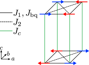
Figure 1: (Color online) Three dimensional collinear phase with antiferromagnetic interlayer exchange $J_{c}$ and biquadratic exchange $J_{\text{bq}}$ between in-plane nearest neighbor sites.

A related question still under debate is the reduced size of the local magnetic moment. Neutron scattering studies find a reduced staggered magnetic moment of (0.31-0.41)$\mu_{\text{B}}$ for LaOFeAs de la Cruz et al. (2008), (0.8-0.9)$\mu_{\text{B}}$ for the 122 pnictide BaFe₂As₂ Ewings et al. (2008), (0.90-0.98)$\mu_{\text{B}}$ for SrFe₂As₂ Zhao et al. (2008a) and 0.8$\mu_{\text{B}}$ for CaFe₂As₂ McQueeney et al. (2008); Zhao et al. (2009). In contrast, theoretical band structure calculations determined much higher values, e.g., up to $2.3\mu_{\text{B}}$ for LaOFeAs Yin et al. (2008).

One conceivable explanation is that the reduction of the local moment is due to a strong frustration within a localized model Si and Abrahams (2008); Yao and Carlson (2008); Uhrig et al. (2009); Ong et al. (2009); Yao and Carlson (2010); Holt et al. (2011). This requires the system to be in the immediate vicinity of a quantum phase transition. But it must be kept in mind that the local magnetic moment depends on matrix elements which are well known only in the limit of localized electrons. Thus, it is possible that the significant reduction of the staggered magnetization is due to electronic effects such as hybridization, spin-orbit coupling and the itineracy of the charges Yildirim (2008); Wu et al. (2008); Lv et al. (2010); Pulikkotil et al. (2010). The bottomline of this argument is that the value of the staggered magnetization is not a stringent constraint for the applicable model for iron pnictides.

I.2 Spatial Anisotropy of Exchange Couplings

Recently, it was shown that a frustrated Heisenberg model in the three dimensional columnar phase Holt et al. (2011) can explain the spin-wave dispersion of CaFe₂As₂ McQueeney et al. (2008); Diallo et al. (2009); Zhao et al. (2009) in the direction perpendicular to the spin stripes and between the layers. However, discrepancies at high energies are present in the direction parallel to the stripes. These discrepancies can be fitted by a Heisenberg model which assumes that the nearest neighbor (NN) coupling $J_{1}$ depends on the spatial direction of the two coupled spins, i.e., one introduces $J_{1a}\gg J_{1b}$ Zhao et al. (2008b); Diallo et al. (2009); Zhao et al. (2009); Han et al. (2009). This is very remarkable since the difference of the orthorhombic distortion between the lattice constants $a$ and $b$ of the columnarly ordered layers is less than 1% Ewings et al. (2008); Diallo et al. (2009), which by far does not give reasons for the large spatial anisotropy of the magnetic exchange. This argument is further supported by the observation that density functional calculations achieve a good description of the pnictides if magnetic columnar order is accounted for. But the consideration of the orthorhombic distortions is only a minor point Han et al. (2009).

Another possible explanation of the spatial anisotropy is the possibility of orbital ordering Singh (2009). But orbital ordering is usually related to higher energies and should lead to clear experimental signatures or theoretical signatures in density-functional calculations which are so far not found.

So it appears that the magnetism itself generates the spatial anisotropy although the original magnetic model is not anisotropic. Indeed, the anisotropic order generates some anisotropic velocities in self-consistent spin-wave theory Uhrig et al. (2009); Holt et al. (2011). But this effect is not sufficient Holt et al. (2011) to account for $J_{1a}\approx 40$ meV and $J_{1b}\approx 0$ meV Zhao et al. (2009); Han et al. (2009).

In order to identify a magnetic process which is able to generate the observed spatial anisotropy one has to go beyond bilinear exchange. This is possible in view of the larger spin value $S\geq 1$. Indeed, significant higher spin exchange processes are inevitable Girardeau and Popovic-Boziv (1977); Mila and Zhang (2000). To be specific, we will consider the biquadratic exchange

$$H_{\text{bq}} =-J_{\text{bq}}\sum\limits_{\langle i,j\rangle}\left(\mathbf{S}_{i}\cdot\mathbf{S}_{j}\right)^{2}$$ (2)

with $J_{\text{bq}}>0$. How does a term such as $H_{\text{bq}}$ influence the magnetic excitations? To obtain a rule of thumb we adopt a simple view and approximate

$$-J_{\text{bq}}\sum\limits_{\langle i,j\rangle}\left(\mathbf{S}_{i}\cdot\mathbf{S}_{j}\right)^{2}\approx-2J_{\text{bq}}\sum\limits_{\langle i,j\rangle}\mathbf{S}_{i}\cdot\mathbf{S}_{j}\langle\mathbf{S}_{i}\cdot\mathbf{S}_{j}\rangle$$

$$+J_{\text{bq}}\sum\limits_{\langle i,j\rangle}\langle\mathbf{S}_{i}\cdot\mathbf{S}_{j}\rangle^{2}.$$ (3)

In the above formula we do not list terms of the types $S_{i}^{(\gamma)}S_{i}^{(\delta)}\langle S_{j}^{(\gamma)}S_{j}^{(\delta)}\rangle$ or $\langle S_{i}^{(\gamma)}S_{i}^{(\delta)}\rangle\langle S_{j}^{(\gamma)}S_{j}^{(\delta)}\rangle$ because both would only contribute for $\gamma=\delta\in\{x,y,z\}$ and then their sum over all spin components would merely yield trivial constants. In the direction of alternating spin orientation one has $\langle\mathbf{S}_{i}\cdot\mathbf{S}_{j}\rangle<0$ so that the biquadratic term effectively strengthens the bilinear antiferromagnetic exchange: $J_{1a}^{\text{eff}}>J_{1}$. In contrast, in the direction of parallel spin orientation one has $\langle\mathbf{S}_{i}\cdot\mathbf{S}_{j}\rangle>0$ so that the biquadratic term effectively weakens the bilinear antiferromagnetic exchange: $J_{1b}^{\text{eff}}<J_{1}$. Hence a NN biquadratic exchange appears to generate a spatial anisotropy purely from the magnetic order. One of the two main goals of the present paper is to substantiate this argument phenomenologically.

If derived from extended standard Hubbard models the biquadratic terms are of higher order in the intersite hoppings than the bilinear exchange coupling which implies that it is actually small relative to the bilinear exchange Mila and Zhang (2000). The exception is a situation where the bilinear terms are subject to near cancellation of antiferromagnetic and ferromagnetic contributions.

In the pnictides, even the undoped systems are conducting bad metals. It is known that close to the transition from localized to conducting systems higher order processes start playing a significant role. For instance, the cyclic exchange in one-band Hubbard models becomes as large as 20% of the NN exchange, see for instance Ref. Hamerla et al., 2010 and references therein.

In addition, evidence for biquadratic exchange has already appeared in calculations based on the self-consistent local spin-density approximation (LSDA) by Yaresko et al. Yaresko et al. (2009). Results for the dependence of the ground state energy of two intercalated Néel ordered sublattices on the angle $\varphi$ between their sublattice magnetizations are displayed in Fig. 2. With bilinear exchanges no dependence is expected at all. The results for BaFe₂As₂ and LaOFeAs are are reproduced in Fig. 2. The dependence of $E(\varphi)=A\cdot\sin^{2}\varphi$ on $\varphi$ is compelling evidence for a biquadratic NN exchange because a dependence $\propto\sin^{2}\varphi$ does not occur in the frustrated $J_{1}$-$J_{2}$ Heisenberg model. Appropriate values for the biquadratic exchange are determined from the maximum $E(\varphi=90^{\circ})$ in Fig. 2 for $S=1$. The obtained values are

$$J_{\text{bq}} =21.5\ \text{meV}\ \text{for LaOFeAs},$$ (4a)

$$J_{\text{bq}} =10.1\ \text{meV}\ \text{for BaFe${}_{2}$As${}_{2}$},$$ (4b)

which are indeed sizeable in view of $J_{1}$ of the order $40$ meV.

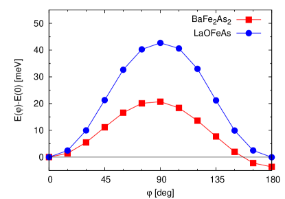
Figure 2: (Color online) Dependence of the ground state energy on the relative angle $\varphi$ between the two sublattice magnetizations on the two intercalated Néel lattices, after Ref. Yaresko et al., 2009.

In general, the electronic situation in the iron pnictides is very complex Wu et al. (2008); up to five bands are important Yildirim (2008); Yin et al. (2008). The appropriate electronic description has not yet been identified Graser et al. (2010); Wu et al. (2008); Schickling et al. (2011) and thus it is presently not possible to discuss the relative size of a biquadratic exchange reliable. Hence we adopt here the phenomenological approach to take the microscopic arguments as evidence for the existence of such a biquadratic exchange. Next, the aim will be to derive the size of $J_{\text{bq}}$ from fits to experiment.

I.3 Methods

Based on our previous work Uhrig et al. (2009); Holt et al. (2011), we study the $J_{1}$-$J_{2}$-$J_{c}$ model in the three-dimensional phase with columnar spin order. First, we discuss the “critical” value of $x=J_{1}/J_{2}$ where the columnar phase ceases to exist and the corresponding two scenarios for this instability. Furthermore, we extend the $J_{1}$-$J_{2}$-$J_{c}$ model by the biquadratic exchange discussed above. To this end, an appropriate mean-field decoupling has to be introduced which is able to tackle biquadratic exchange as well.

To establish a reliable mean-field approach we employ the Dyson-Maleev as well as the Schwinger bosons representation. To gauge the resulting decoupling schemes both are applied to the two dimensional Néel phase of a NN bilinear Heisenberg model plus biquadratic exchange for $S=1$. Then, the successful decoupling is applied to the three dimensional columnar phase with biquadratic exchange for $1\leq S\leq 2$. General results are discussed before we apply the model to CaFe₂As₂.

II Scenarios for the $J_{1}$-$J_{2}$-$J_{c}$ model

Here we discuss two fundamental scenarios for the instability of spatially anisotropic phases of magnetic long-range order. We do not consider first-order transitions to other phases; in particular we do not aim to discuss the existence of possible intermediate disordered phases between Néel and columnar phase. Instead we focus on how the columnar phase can become unstable towards fluctuations. We stress that the self-consistent spin-wave theory is expected to yield reliable results for $S\geq 1>1/2$ and dimension $d=3>2$ since its results are already very good Singh et al. (2003); Uhrig et al. (2009) for $S=1/2$ and $d=2$.

It is generally agreed that the staggered magnetization in the columnar phase of two-dimensional $J_{1}$-$J_{2}$ model can take any possible value provided an adequate fine-tuning of the coupling ratio $x=J_{1}/J_{2}$ is performed Uhrig et al. (2009); Smerald and Shannon (2010). Here we point out that this is no longer true in the presence of an interlayer coupling $J_{c}$. The quantitative aspects, though not the qualitative ones, depend strongly on the spin $S$.

Passing from two to three dimensions the additional coupling between the columnarly ordered planes cuts off the logarithmic divergence of the Goldstone modes Smerald and Shannon (2010). Thus, in three dimensions the staggered magnetization may no longer adopt any arbitrary value $\geq 0$ even if the ratio $x=J_{1}/J_{2}$ is increased towards 2. Instead, there can be a finite minimum value of the staggered magnetization whose value depends on the relative interlayer coupling $\mu=J_{c}/J_{1}$.

There are two possible outcomes upon $x\to 2$. If the value of $\mu$ is not too large, it is still possible to drive the magnetization to zero while all the three different spin-wave velocities remain finite. But for larger values of $\mu$ the magnetization remains finite while the smallest of the spin-wave velocities vanishes Holt et al. (2011). Thus, we face two qualitatively different scenarios. They can easily be distinguished in plotting the ratio $v_{b}/v_{a}$ versus the staggered magnetization $m_{\text{st}}$. The results for $S=1/2$ and $S=1$ are shown in Fig. 3.

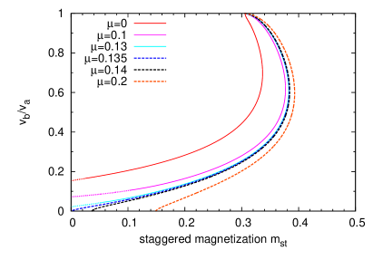
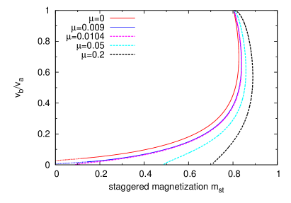
Figure 3: (Color online) Ratio $v_{b}/v_{a}$ as a function of $m_{\text{st}}$ for $S=1/2$ (upper panel) and $S=1$ (lower panel). The curves either end on the ordinate, i.e, for zero staggered magnetization, or on the abscissa, i.e., for zero spin-wave velocity $v_{b}<v_{c}<v_{a}$. Thus, two qualitatively different instabilities emerge naturally. The solid lines correspond to the magnetization-driven scenario (vanishing magnetization) while the dashed lines correspond to the velocity-driven scenario (vanishing spin-wave velocity). The dotted lines are extrapolations in the magnetization-driven scenario.

In the first scenario (solid lines), the ratio $v_{b}/v_{a}$ always stays positive and the instability of the phase is marked by the staggered magnetization $m_{\text{st}}$ going to zero. Thus, we call this scenario the magnetization-driven scenario because the breakdown of the columnar phase is driven by the vanishing magnetic long-range order. The numerical evaluation of the three dimensional integrals becomes very difficult close to $m_{\text{st}}=0$ so that the solid curves in Fig. 3 can only be computed down to some small finite value of the staggered magnetization. Beyond this point they are extrapolated as depicted by the dotted curves. In this way the phase diagrams of the $J_{1}$-$J_{2}$-$J_{c}$ Heisenberg model in Ref. Holt et al., 2011 were determined.

The dashed lines in Fig. 3 correspond to the second scenario. We call it the velocity-driven scenario because the vanishing of the spin-wave velocity $v_{b}$ marks the instability of the columnar phase. If $x$ were taken infinitesimally higher, $v_{b}^{2}$ would become negative so that no physically meaningful mean-field model would be found. The staggered magnetization $m_{\text{st}}$ stops at this point at a finite positive value. This finite positive value of the staggered magnetization may appear surprising because it signifies that the magnetic long-range order still persists even though the columnar phase ceases to exist because its excitations become unstable.

In the case of $S=1/2$, the transition from the magnetization- to the velocity-driven scenario occurs for $\mu_{\text{mv}}\approx 0.134$. Thus, the magnetization-driven scenario applies in the range $0\leq\mu\lesssim 0.134$. The precise value of $\mu$ where the magnetization-driven scenario switches over to the velocity-driven scenario corresponds to the curve in the $v_{b}/v_{a}$-$m_{\text{st}}$ plane which ends at the origin. If the interlayer coupling is increased beyond $\mu_{\text{mv}}$, the velocity-driven scenario applies.

For $S=1$, the change from one scenario to the other occurs roughly at $\mu_{\text{mv}}\approx 0.01$, see lower panel of Fig. 3. Thus, the magnetization-driven scenario for $S=1$ persists in the range of $0\leq\mu\lesssim 0.01$, which is a much smaller region compared to the case for $S=1/2$. We stress, however, that there is no qualitative difference between $S=1/2$ and $S=1$. For even larger spin values the magnetization-driven scenario will only apply for a quickly decreasing range of interplane couplings $\mu=J_{c}/J_{1}$. This is due to the fact that the instability of the columnar phase shifts for increasing spin very quickly to where it occurs classically Chandra and Doucot (1988), i.e., for $x=2$. Since larger and larger spins correspond to a more and more classical behavior it is not astounding that one has to draw nearer and nearer to the logarithmic divergence of the quantum fluctuations in order for them to become important. Hence $S\to\infty$ implies an exponential convergence $x\to 2$ and $\mu_{\text{mv}}\to 0$.

We emphasize that the full discussion of the instability of the columnar phase requires the consideration of first order transitions as well. This is beyond the scope of the present paper because we do not know the phase into which the columnar phase becomes unstable. It may be a disordered phase, but in view of the larger spin $S\geq 1$ and the dimension $d=3$ we expect that an intermediate phase exists only for a very small parameter region.

From the knowledge for $S=1/2$ and $S=1$ in two and three dimensions Singh et al. (1999); Kotov et al. (1999); Sushkov et al. (2001); Singh et al. (2003); Schmalfuß et al. (2006); Bishop et al. (2008); Majumdar (2010, 2011a) we presume that the magnetization-driven scenarios eventually becomes a weak first order transition to an intermediate phase existing only within a small parameter region. Further, we expect that the velocity-driven scenario becomes a strong first order transition to the Néel phase.

III Biquadratic Exchange in the 2D Néel Phase

In this section, we study the effects of a biquadratic exchange (2) on the simple NN Heisenberg model ($J_{2}=0$) with $S=1$ on the square lattice. The aim is to establish a reliable mean-field description.

We apply the Schwinger bosons as well as the Dyson-Maleev representation to the model and introduce the corresponding mean-field approximation. Our aim is to study the influence of the biquadratic exchange on the dispersion of the spin-waves. The findings are checked against results obtained by exact diagonalization and series expansion.

The Hamiltonian under study reads

$$H= J\sum\limits_{\langle i,j\rangle}\mathbf{S}_{i}\cdot\mathbf{S}_{j}-J_{\text{bq}}\sum\limits_{\langle i,j\rangle}\left(\mathbf{S}_{i}\cdot\mathbf{S}_{j}\right)^{2},$$ (5)

where $J,J_{\text{bq}}>0$. The brackets $\left<i,j\right>$ indicate the summation over NN sites.

III.1 Dyson-Maleev representation

First, we apply the Dyson-Maleev transformation Dyson (1956a, b); Maleev (1958) to the Hamiltonian (5). On sublattice $A$, the expression of the spin operators in terms of bosonic operators reads

$$S^{+}_{i} =b^{\dagger}_{i}\left(2S-\hat{n}^{\phantom{\dagger}}_{i}\right)$$ (6a)

$$S^{-}_{i} =b_{i}^{\phantom{\dagger}}$$ (6b)

$$S^{z}_{i} =-S+\hat{n}_{i}^{\phantom{\dagger}}.$$ (6c)

After a $\pi$-rotation of the spins around the $x$-axis, the transformation on sublattice $B$ is given by

$$S^{+}_{i} =b^{\dagger}_{i}$$ (7a)

$$S^{-}_{i} =\left(2S-\hat{n}^{\phantom{\dagger}}_{i}\right)b_{i}^{\phantom{\dagger}}$$ (7b)

$$S^{z}_{i} =-S+\hat{n}_{i}^{\phantom{\dagger}}.$$ (7c)

The complete Hamiltonian in the Dyson-Maleev representation is given in the Appendix. In preparation of the decoupling we introduce the expectation values

$$n :=\left\langle b^{\dagger}_{i}b_{i}^{\phantom{\dagger}}\right\rangle=\left\langle b^{\dagger}_{j}b^{\phantom{\dagger}}_{j}\right\rangle$$ (8a)

$$a :=\left\langle b^{\dagger}_{i}b_{j}^{\dagger}\right\rangle=\left\langle b^{\phantom{\dagger}}_{i}b^{\phantom{\dagger}}_{j}\right\rangle,$$ (8b)

where $i,j$ are NN sites with $i\in A$ and $j\in B$. All other expectation values vanish because of the conservation of the total $S^{z}$ component $\sum_{i}S^{z}_{i}$. For simplicity, we assume that the expectation values are real. The high-order terms are decoupled according to Wick’s theorem Fetter and Walecka (1971). Neglecting all constant terms the mean-field Hamiltonian is given by

$$H^{\text{MF}} =\widetilde{J}_{\text{DM}}(\alpha)\left(S-\alpha\right)\sum\limits_{\langle i,j\rangle}\left(\hat{n}_{i}+\hat{n}_{j}+b^{\dagger}_{i}b^{\dagger}_{j}+b^{\phantom{\dagger}}_{i}b^{\phantom{\dagger}}_{j}\right),$$ (9)

where the subscript DM stands for Dyson-Maleev and should not be confused with Dzyaloshinskii-Moriya. We define

$$\begin{split}\widetilde{J}_{\text{DM}}(\alpha)&:=J+\frac{J_{\text{bq}}}{S-\alpha}\left[2S^{3}-2S^{2}(1+5\alpha)\right.\\ &\left.+S(18\alpha^{2}+8\alpha+1)-12\alpha^{3}-9\alpha^{2}-2\alpha\right]\end{split}$$ (10)

where the new parameter

$$\alpha :=n+a$$ (11)

has been introduced for convenience. The parameter $\alpha$ has to be determined self-consistently, see below. The mean-field Hamiltonian (9) can easily be transformed into momentum space where it can be diagonalized using a standard Bogoliubov transformation. The diagonalized Hamiltonian reads

$$H^{\text{MF}} =\sum\limits_{\mathbf{k}\in\text{BZ}}\omega_{\mathbf{k}}^{\phantom{\dagger}}\beta^{\dagger}_{\mathbf{k}}\beta^{\phantom{\dagger}}_{\mathbf{k}}+E^{\text{MF}}.$$ (12)

We stress that the full Brillouin zone (BZ), i.e., $-\pi<k_{\gamma}\leq\pi$ for each component $\gamma\in\{a,b\}$, is used here and hereafter. This is done for simplicity because full translational invariance holds and there is only one mode per $k$ point; but it does not have a definite value of its total $S_{z}$ component. The dispersion is given by

$$\omega_{\mathbf{k}} =2\widetilde{J}_{\text{DM}}(\alpha)\left(S-\alpha\right)\widetilde{\omega}_{\mathbf{k}}$$ (13a)

$$\widetilde{\omega}_{\mathbf{k}}^{2} =4-\left(\cos k_{a}+\cos k_{b}\right)^{2}$$ (13b)

and the ground state energy by

$$E^{\text{MF}} =\widetilde{J}_{\text{DM}}(\alpha)\left(S-\alpha\right)\widetilde{E}^{\text{MF}}$$ (14a)

$$\widetilde{E}^{\text{MF}} =\sum\limits_{\mathbf{k}\in\text{BZ}}\left(\widetilde{\omega}_{\mathbf{k}}-2\right).$$ (14b)

The gapless excitations at $k=(1,1)$ which is the magnetic ordering vector of the Néel phase and at $k=(0,0)$ are the expected Goldstone modes, because the ground state of the system has broken symmetry Lange (1966). The existence of these gapless excitations is guaranteed by the systematic expansion in $1/S$. We draw the reader’s attention to the fact that this argument ensures massless modes only for the systematic expansion, i.e., for a particular value of $\alpha$. But it turns out that the vanishing of the energy of the Goldstone modes does not depend on the precise numbers of the expectation values so that it does not matter whether the expansion is performed systematically or self-consistently.

The self-consistent equation for the parameter $\alpha$ is found by comparing (9) with the mean-field ground state energy (14) per site yielding $\alpha=(1/2)\widetilde{E}^{\text{MF}}/N$ if $N$ is the number of sites. Hence we have in the thermodynamic limit $N\to\infty$

$$\alpha =\frac{1}{4}\frac{1}{\left(2\pi\right)^{2}}\iint\limits_{\text{BZ}}\mathrm{d}^{2}k\;(\widetilde{\omega}_{\mathbf{k}}-2)$$ (15a)

$$=-0.0789737105.$$ (15b)

One integration in (15b) can be done analytically, the second one with any computer algebra system. Note that due to the simplicity of the system no real self-consistency needs to be determined; $\alpha$ can be computed directly.

III.2 Schwinger boson representation

Here we apply the Schwinger boson representation Auerbach (1994) to the Hamiltonian (5). The spin operators are expressed as

$$S^{+}_{i} =a^{\dagger}_{i}b^{\phantom{\dagger}}_{i}$$ (16a)

$$S^{-}_{i} =b^{\dagger}_{i}a^{\phantom{\dagger}}_{i}$$ (16b)

$$S^{z}_{i} =\frac{1}{2}\left(a^{\dagger}_{i}a_{i}^{\phantom{\dagger}}+b^{\dagger}_{i}b_{i}^{\phantom{\dagger}}\right).$$ (16c)

The constraint

$$a^{\dagger}_{i}a^{\phantom{\dagger}}_{i}+b^{\dagger}_{i}b_{i}^{\phantom{\dagger}} =2S$$ (17)

restricts the infinite bosonic Hilbert space to the relevant physical subspace of the spin $S$. In this way, the Hamiltonian (5) is rewritten as

$$\begin{split}H&=-\frac{J}{2}\sum\limits_{\langle i,j\rangle}\left(A^{\dagger}_{ij}A^{{\phantom{\dagger}}}_{ij}-2S^{2}\right)\\ &\quad-\frac{J_{\text{bq}}}{4}\sum\limits_{\langle i,j\rangle}\left(4S^{4}-4S^{2}A^{\dagger}_{ij}A^{{\phantom{\dagger}}}_{ij}+\left(A^{\dagger}_{ij}A^{{\phantom{\dagger}}}_{ij}\right)^{2}\right),\end{split}$$ (18)

where the bond operators

$$A^{\dagger}_{ij} =a^{\dagger}_{i}a^{\dagger}_{j}+b^{\dagger}_{i}b^{\dagger}_{j}$$ (19a)

$$A^{{\phantom{\dagger}}}_{ij} =a^{{\phantom{\dagger}}}_{i}a^{{\phantom{\dagger}}}_{j}+b^{{\phantom{\dagger}}}_{i}b^{{\phantom{\dagger}}}_{j}$$ (19b)

are used. They connect adjacent sites on the different sublattices with $i\in A$ and $j\in B$.

The mean-field approximation in terms of the bond operators is based on an expansion in the inverse number of boson flavors $1/\mathcal{N}$ Auerbach (1994); Auerbach and Arovas (1988); Arovas and Auerbach (1988). Thus, we intermediately extend to $\mathcal{N}$ Schwinger boson flavors to justify the approximation. For $\mathcal{N}$ flavors, the bilinear term reads

$$\mathbf{S}_{i}\cdot\mathbf{S}_{j} =-\frac{1}{\mathcal{N}}A^{\dagger}_{ij}A^{\phantom{\dagger}}_{ij}+S^{2}$$ (20)

with the generalized bond operators

$$A^{\dagger}_{ij} =\sum\limits_{m=1}^{\mathcal{N}}a^{\dagger}_{i,m}a^{\dagger}_{j,m}$$ (21a)

$$A^{{\phantom{\dagger}}}_{ij} =\sum\limits_{m=1}^{\mathcal{N}}a^{\phantom{\dagger}}_{i,m}a^{\phantom{\dagger}}_{j,m}$$ (21b)

and the constraint

$$\sum\limits^{\mathcal{N}}_{m=1}a^{\dagger}_{i,m}a^{{\phantom{\dagger}}}_{i,m} =\mathcal{N}S.$$ (22)

We define the expectation value

$$A:=\langle A^{{\phantom{\dagger}}}_{ij}\rangle=\langle A^{\dagger}_{ij}\rangle\ \geq 0,$$ (23)

which is proportional to $\mathcal{N}$ according to the generalized constraint (22). Hence, the bilinear term is decoupled according to

$$\begin{split}\left.\mathbf{S}_{i}\cdot\mathbf{S}_{j}\right|_{\text{MF}}&\approx-\frac{1}{\mathcal{N}}\left(AA^{\dagger}_{ij}+\operatorname{h.c.}\right),\end{split}$$ (24)

where we only keep the leading order $\mathcal{O}\left((1/\mathcal{N})^{0}\right)$ omitting constants.

In complete analogy, the quartic term of bond operators is decoupled in leading order by

$$\frac{1}{\mathcal{N}^{2}}\left(A^{\dagger}_{ij}A^{{\phantom{\dagger}}}_{ij}\right)\cdot\left(A^{\dagger}_{ij}A^{{\phantom{\dagger}}}_{ij}\right) \approx\frac{2A^{2}}{\mathcal{N}^{2}}\left(A^{\dagger}_{ij}A+AA^{{\phantom{\dagger}}}_{ij}\right).$$ (25)

The factor 2 is a consequence of Wicks’s theorem, as there are two possibilities to contract the operators $A^{\dagger}_{ij}$ or $A^{{\phantom{\dagger}}}_{ij}$. Thus, the mean-field decoupling of the entire biquadratic term reads

$$\left.\left(\mathbf{S}_{i}\cdot\mathbf{S}_{j}\right)^{2}\right|_{\text{MF}} \approx-\frac{2S^{2}}{\mathcal{N}}A\left(1-\frac{A^{2}}{\mathcal{N}S^{2}}\right)\left(A^{\dagger}_{ij}+A^{{\phantom{\dagger}}}_{ij}\right).$$ (26)

Since $A\propto\mathcal{N}S$, $A^{2}>\mathcal{N}S^{2}$ holds so that the biquadratic term yields a positive contribution in total. Due to the prefactor $-J_{\text{bq}}$, cf. Eq. (18), the biquadratic term enhances the bilinear one (24).

Returning to $\mathcal{N}=2$, the mean-field Hamiltonian is finally given by

$$H^{\text{MF}} =-B\sum\limits_{\langle i,j\rangle}\left(A^{\dagger}_{ij}+\operatorname{h.c.}\right)+\lambda\sum\limits_{i}\left(a^{\dagger}_{i}a_{i}^{{\phantom{\dagger}}}+b^{\dagger}_{i}b_{i}^{{\phantom{\dagger}}}\right),$$ (27)

where

$$B :={A\widetilde{J}_{\text{SB}}(A)}/{2}$$ (28)

$$\widetilde{J}_{\text{SB}}(A) :=J-2J_{\text{bq}}S^{2}\left(1-{A^{2}}/{(2S^{2})}\right).$$ (29)

The Lagrange multiplier $\lambda$ is introduced to enforce the constraint (17) on average. In the symmetry broken phase at zero temperature, $\lambda$ is fixed to the value

$$\lambda =4B=2\widetilde{J}_{\text{SB}}\left(A\right)A$$ (30)

in order to retrieve massless Goldstone bosons. In momentum space, the mean-field Hamiltonian (27) is diagonalized by a standard Bogoliubov transformation leading to the dispersion and the ground state energy

$$\omega_{\mathbf{k}} =\sqrt{\lambda^{2}-\left(4B\left(\cos k_{a}+\cos k_{b}\right)\right)^{2}}$$ (31a)

$$E^{\text{MF}} =\sum\limits_{\mathbf{k}\in\text{BZ}}\left(\omega_{\mathbf{k}}-\lambda\right).$$ (31b)

The self-consistency equations for the parameters $A$ and $\lambda$ are given by

$$2S =\frac{1}{N}\frac{\partial E^{\text{MF}}}{\partial\lambda}$$ (32a)

$$-4A =\frac{1}{N}\frac{\partial E^{\text{MF}}}{\partial B}\,.$$ (32b)

These two equations can be combined to yield $A$ in the symmetry broken phase

$$A =2S+1-\frac{1}{2}\iint\limits_{\text{BZ}}\frac{\mathrm{d}^{2}k}{\left(2\pi\right)^{2}}\sqrt{4-\left(\cos k_{a}+\cos k_{b}\right)^{2}}$$ (33)

in the thermodynamic limit. Note that the massless Goldstone modes are again guaranteed by the systematic expansion which is here done in the inverse number of flavors $1/\mathcal{N}$. As for the Dyson-Maleev mean-field approach the expansion can also be done self-consistently without spoiling the Goldstone theorem because the precise number of the expectation value $A$ does not matter for this qualitative aspect. For $S=1$, the calculated value is

$$A =2.1579474210$$ (34)

which corresponds to $2(1-\alpha)$ from the Dyson-Maleev calculation. Thus the obtained dispersions are identical for zero biquadratic exchange because then $\widetilde{J}_{\text{SB}}=\widetilde{J}_{\text{DM}}$ holds.

III.3 Results

We are interested in the influence of the biquadratic exchange on the excitation energies. Thus the ratios of the dispersions with and without biquadratic exchange is an appropriate quantity. Since the shape of the dispersions is the same for the Dyson-Maleev and the Schwinger boson representation, no more quantities need to be compared. This ratio depends linearly on the coupling ratio $\nu:=J_{\text{bq}}/J$, see Eqs. (10) and (29). This behavior is depicted in Fig. 4 and the corresponding slopes are given in Tab. 1.

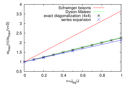
Figure 4: (Color online) Influence of the biquadratic exchange on the excitation energies in the 2D Néel phase ($S=1$). The dashed lines are fits to the corresponding data points. Note the almost perfect straight lines obtained in exact diagonalization and in series expansion.

method	slopes
Schwinger bosons	2.65674
Dyson-Maleev	1.27708
exact diagonalization (4x4)	1.24505
series expansion	1.13423

Table 1: (Color online) Slopes for the influence of the biquadratic exchange on the maximum excitation energy relative to the one without biquadratic exchange, see Fig. 4 for the data from which the slopes are fitted for exact diagonalization and series expansion.

The mean-field results for the 2D Néel phase with biquadratic exchange are checked to the results obtained by other methods. In detail, the excitation energies can be calculated by an exact diagonalization of the Hamiltonian (5) on a finite 4x4 lattice Raas (2009) and by series expansion Oitmaa et al. (2006); Oitmaa (2009). For both methods, the slope is determined by a linear fit, see Fig. 1. All results are compared in Tab. 1 and displayed in Fig. 4. The data points are the maximum excitation energies normalized to the maximum without biquadratic exchange.

The Schwinger bosons result immediately catches one’s eye because the slope is far too large by a factor greater than two. In contrast, the Dyson-Maleev result matches very well with the exact diagonalization. Of course, the exact diagonalization data is hampered by finite size effects even though they are only moderate because we consider the ratio of the maximum of the dispersion. The slope of the series expansion, which is essentially exact, is slightly smaller. The deviation of the Dyson-Maleev slope from the series expansion is in the range of 10-15%, which is well acceptable for a mean-field approach applied to complicated terms made from eight bosonic operators. Extending the model to three dimensions, we expect the result to improve because mean-field approximations generally become the more accurate the higher the number of dimensions. Therefore, we choose to employ to the Dyson-Maleev representation and the corresponding mean-field approximation in the study of the columnar phase.

Discrepancies of the Schwinger boson mean-field theory to other treatments appeared already without biquadratic exchange when the theory was introduced by Auerbach and Arovas Auerbach and Arovas (1988); Arovas and Auerbach (1988). In their calculations, the mean-field free energy exceeded previous results by a factor of 2 and the sum rule of the dynamic structure factor exceeded its exact value by a factor of $3/2$.

In the mean-field approximation for Schwinger bosons, we treat both Schwinger bosons on a site as independent. Thus, the constraint (17) is violated because a change in the occupation of the $a$ boson should always be connected to a change of the occupation of the $b$ boson on the same lattice site. Hence, we suggest that the additional factors appear because of the missed suppression of fluctuations of the boson number due to the constraint. Since the biquadratic exchange can be roughly viewed as a bilinear exchange multiplied by a NN expectation value, see Eq. (3), it is comprehensible that the slope of the Schwinger boson mean-field result is too large by about a factor of 2 because the NN expectation value is overestimated by this factor Auerbach and Arovas (1988).

IV 3D columnar phase with biquadratic exchange

As explained in the Introduction we advocate that a localized spin model for the pnictides has to comprise a biquadratic term in order to account for the spatial anisotropy of the spin-wave velocities measured by inelastic neutron scattering (INS) and computed by density functional theory. Thus, we set out to investigate the Hamiltonian

$$\begin{split}H&=J_{1}\sum\limits_{\langle i,j\rangle}\mathbf{S}_{i}\cdot\mathbf{S}_{j}+J_{2}\sum\limits_{\langle\langle i,j\rangle\rangle}\mathbf{S}_{i}\cdot\mathbf{S}_{j}\\ &\quad\quad+J_{c}\sum\limits_{[i,j]}\mathbf{S}_{i}\cdot\mathbf{S}_{j}-J_{\text{bq}}\sum\limits_{\langle i,j\rangle}\left(\mathbf{S}_{i}\cdot\mathbf{S}_{j}\right)^{2},\end{split}$$ (35)

where a NN in-plane biquadratic exchange ($J_{\text{bq}}>0$) is introduced. The brackets $\left<i,j\right>$ and $\left<\left<i,j\right>\right>$ correspond to in-plane nearest and next-nearest neighbor sites, while the bracket $[i,j]$ indicates the exchange between interplane nearest neighbor sites. The very small orthorhombic distortion in the columnarly ordered layers is neglected. Justified by the checks in the previous Section, we employ the Dyson-Maleev representation and the ensuing mean-field approximation. In order to establish our notation we provide a brief derivation of the spin-wave dispersion and the self-consistency equations. For further details the reader is referred to Ref. Stanek, 2010.

For the mean-field decoupling, the following parameters are needed:

• average occupation number per lattice site

  $$n :=\left\langle b^{\dagger}_{i}b_{i}^{\phantom{\dagger}}\right\rangle=\left\langle b^{\dagger}_{j}b^{\phantom{\dagger}}_{j}\right\rangle,$$ (36a)

• in-plane NN antiparallel spin orientation perpendicular to the spin stripes ($a$-direction)

  $$a_{1} :=\left\langle b^{\dagger}_{i}b_{j}^{\dagger}\right\rangle=\left\langle b^{\phantom{\dagger}}_{i}b^{\phantom{\dagger}}_{j}\right\rangle$$ (36b)

• interlayer NN antiparallel spin orientation ($c$-direction)

  $$a_{c} :=\left\langle b^{\dagger}_{i}b_{j}^{\dagger}\right\rangle=\left\langle b^{\phantom{\dagger}}_{i}b^{\phantom{\dagger}}_{j}\right\rangle$$ (36c)

• in-plane next-nearest neighbor (NNN) antiparallel spin orientation

  $$a_{2} :=\left\langle b^{\dagger}_{i}b_{j}^{\dagger}\right\rangle=\left\langle b^{\phantom{\dagger}}_{i}b^{\phantom{\dagger}}_{j}\right\rangle$$ (36d)

• in-plane NN parallel spin orientation parallel to the spin stripes ($b$-direction)

  $$f :=\left\langle b^{\dagger}_{i}b_{j}^{\phantom{\dagger}}\right\rangle=\left\langle b^{\dagger}_{j}b^{\phantom{\dagger}}_{i}\right\rangle$$ (36e)

It turns out to be advantageous to introduce the combined parameters $\alpha_{1}$, $\alpha_{2}$, $\alpha_{c}$ and $\beta$ according to

$$\alpha_{1} :=n+a_{1}$$ (37a)

$$\alpha_{c} :=n+a_{c}$$ (37b)

$$\alpha_{2} :=n+a_{2}$$ (37c)

$$\beta :=n-f.$$ (37d)

The values of these parameters are determined by the self-consistency equations given below.

Thereby, the mean-field decoupling of the Hamiltonian (35) reads

$$H =H_{\perp}+H_{\parallel}+H_{c}+H_{\text{NNN}}$$ (38a)

$$H_{\perp} =J_{2}x_{1a}\left(S-\alpha_{1}\right)\sum\limits_{\langle i,j\rangle}\left(\hat{n}^{\phantom{\dagger}}_{i}+\hat{n}^{\phantom{\dagger}}_{j}+b^{\dagger}_{i}b^{\dagger}_{j}+b^{\phantom{\dagger}}_{i}b^{\phantom{\dagger}}_{j}\right)$$ (38b)

$$H_{\parallel} =-J_{2}x_{1b}\left(S-\beta\right)\sum\limits_{\langle i,j\rangle}\left(\hat{n}_{i}^{\phantom{\dagger}}+\hat{n}^{\phantom{\dagger}}_{j}-b^{\dagger}_{i}b^{\phantom{\dagger}}_{j}-b^{\dagger}_{j}b^{\phantom{\dagger}}_{i}\right)$$ (38c)

$$H_{c} =J_{2}x\mu\left(S-\alpha_{c}\right)\sum\limits_{[i,j]}\left(\hat{n}^{\phantom{\dagger}}_{i}+\hat{n}^{\phantom{\dagger}}_{j}+b^{\dagger}_{i}b^{\dagger}_{j}+b^{\phantom{\dagger}}_{i}b^{\phantom{\dagger}}_{j}\right)$$ (38d)

$$H_{\text{NNN}} =J_{2}\left(S-\alpha_{2}\right)\sum\limits_{\langle\langle i,j\rangle\rangle}\left(\hat{n}^{\phantom{\dagger}}_{i}+\hat{n}^{\phantom{\dagger}}_{j}+b^{\dagger}_{i}b^{\dagger}_{j}+b^{\phantom{\dagger}}_{i}b^{\phantom{\dagger}}_{j}\right)$$ (38e)

with $x:=J_{1}/J_{2}$, $\mu:=J_{c}/J_{1}$, $\nu:=J_{\text{bq}}/J_{1}$ and

$$x_{1a} :=x+\frac{x\nu}{S-\alpha_{1}}\big{[}2S^{3}-2S^{2}(1+5\alpha_{1})+$$

$$\qquad S(18\alpha_{1}^{2}+8\alpha_{1}+1)-12\alpha_{1}^{3}-9\alpha_{1}^{2}-2\alpha_{1}\big{]}$$ (39a)

$$x_{1b} :=x-\frac{x\nu}{S-\beta}\big{[}2S^{3}-2S^{2}\left(1+5\beta\right)+$$

$$\qquad S(18\beta^{2}+8\beta)-12\beta^{3}-9\beta^{2}-\beta\big{]}.$$ (39b)

The mean-field Hamiltonian (38) is easily transformed into momentum space and diagonalized by a standard Bogoliubov transformation. Thereby, the spin-wave dispersion

$$\omega_{\mathbf{k}} :=2\sqrt{A_{\mathbf{k}}^{2}-B_{\mathbf{k}}^{2}}$$ (40)

is obtained with

$$A_{\mathbf{k}} :=J_{2}[2(S-\alpha_{2})+x_{1a}(S-\alpha_{1})+$$

$$\qquad x\mu(S-\alpha_{c})+x_{1b}(S-\beta)(\cos k_{b}-1)]$$ (41a)

$$B_{\mathbf{k}} :=J_{2}[x_{1a}(S-\alpha_{1})\cos k_{a}+x\mu(S-\alpha_{c})\cos k_{c}+$$

$$\qquad 2(S-\alpha_{2})\cos k_{a}\cos k_{b}].$$ (41b)

The components $k_{a}$, $k_{b}$ and $k_{c}$ of the momentum vector $\mathbf{k}$ are directed along the crystal axes as shown in Fig. 1. The dispersion is gapless at $k=(0,0,0)$ and $k=(1,0,1)$ corresponding to the required Goldstone modes Uhrig et al. (2009); Holt et al. (2011). Note that this feature is again guaranteed by the systematic expansion in the inverse spin $1/S$. As for the Néel phase the expansion can also be done self-consistently without spoiling the Goldstone theorem because the precise numbers of the expectation values do not matter for this qualitative aspect. But we consider this a highly non-trivial aspect in view of the four different quantum corrections occuring here.

For small momenta, the dispersion (40) can be expanded

$$\omega_{\mathbf{k}} \approx\sqrt{v_{a}^{2}k_{a}^{2}+v_{b}^{2}k_{b}^{2}+v_{c}^{2}k_{c}^{2}}$$ (42)

and one obtains the spin-wave velocities

$$v_{a}^{2} =(2J_{2})^{2}[2(S-\alpha_{2})+x_{1a}(S-\alpha_{1})+x\mu(S-\alpha_{c})]\times$$

$$[2(S-\alpha_{2})+x_{1a}(S-\alpha_{1})]$$ (43a)

$$v_{b}^{2} =(2J_{2})^{2}[2(S-\alpha_{2})+x_{1a}(S-\alpha_{1})+x\mu(S-\alpha_{c})]\times$$

$$[2(S-\alpha_{2})-x_{1b}(S-\beta)]$$ (43b)

$$v_{c}^{2} =(2J_{2})^{2}[2(S-\alpha_{2})+x_{1a}(S-\alpha_{1})+x\mu(S-\alpha_{c})]\times$$

$$x\mu(S-\alpha_{c}).$$ (43c)

The parameters of the quantum corrections are determined from the self-consistency equations in the thermodynamic limit

$$\alpha_{1} =\frac{1}{2}\frac{1}{\left(2\pi\right)^{3}}\iiint\limits_{\text{BZ}}\mathrm{d}^{3}k\ \frac{A_{\mathbf{k}}-B_{\mathbf{k}}\cos k_{a}}{\sqrt{A_{\mathbf{k}}^{2}-B_{\mathbf{k}}^{2}}}-\frac{1}{2}$$ (44a)

$$\alpha_{c} =\frac{1}{2}\frac{1}{\left(2\pi\right)^{3}}\iiint\limits_{\text{BZ}}\mathrm{d}^{3}k\ \frac{A_{\mathbf{k}}-B_{\mathbf{k}}\cos k_{c}}{\sqrt{A_{\mathbf{k}}^{2}-B_{\mathbf{k}}^{2}}}-\frac{1}{2}$$ (44b)

$$\alpha_{2} =\frac{1}{2}\frac{1}{\left(2\pi\right)^{3}}\iiint\limits_{\text{BZ}}\mathrm{d}^{3}k\ \frac{A_{\mathbf{k}}-B_{\mathbf{k}}\cos k_{a}\cos k_{b}}{\sqrt{A_{\mathbf{k}}^{2}-B_{\mathbf{k}}^{2}}}-\frac{1}{2}$$ (44c)

$$\beta =-\frac{1}{2}\frac{1}{\left(2\pi\right)^{3}}\iiint\limits_{\text{BZ}}\mathrm{d}^{3}k\ \frac{A_{\mathbf{k}}\left(\cos k_{b}-1\right)}{\sqrt{A_{\mathbf{k}}^{2}-B_{\mathbf{k}}^{2}}}-\frac{1}{2},$$ (44d)

where the integrations run over the full Brillouin zone (BZ) as before. The above set of equations is solved by numerical integration and by four-dimensional root finding.

The staggered magnetization $m_{\text{st}}$ is defined as $m_{\text{st}}:=\left<S^{z}_{i}\right>(-1)^{\sigma}$ where $\sigma=0$ for $i\in A$ and $\sigma=1$ for $i\in B$. In the thermodynamic limit, it reads

$$m_{\text{st}} =S+\frac{1}{2}-\frac{1}{2}\frac{1}{\left(2\pi\right)^{3}}\iiint\limits_{\text{BZ}}\mathrm{d}^{3}k\ \frac{A_{\mathbf{k}}}{\sqrt{A_{\mathbf{k}}^{2}-B_{\mathbf{k}}^{2}}}.$$ (45)

IV.1 General Results for $S=1$

We discuss the qualitative aspects for $S=1$ and $\mu=0.25$, which is a generic value for the relative interlayer coupling. The values of the relative biquadratic exchange $\nu$ are chosen in the range of $0.1$ to $0.7$ as motivated in Sect. I.2. For comparison, we also show the results without biquadratic exchange.

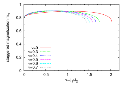
Figure 5: (Color online) Staggered magnetization as a function of $x$ for $S=1$ and $\mu=0.25$. All curves are in the velocity-driven scenario which we presume to signal a strong first order transition to the Néel phase. The magnetization remains finite at the endpoint where the columnar phase ceases to exist, for details see Sect. II.

From the staggered magnetization in Fig. 5, we conclude that the biquadratic exchange destabilizes the columnar phase and drives the critical point towards lower values of $x=J_{1}/J_{2}$. There is only a negligible influence on the maximum value of $m_{\text{st}}$, which is also shifted further left.

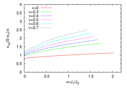
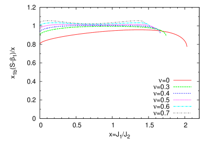
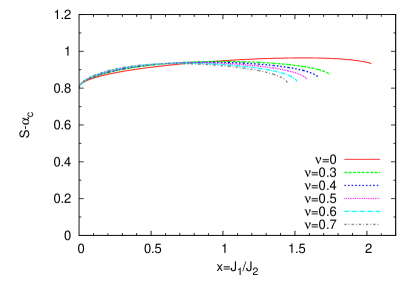
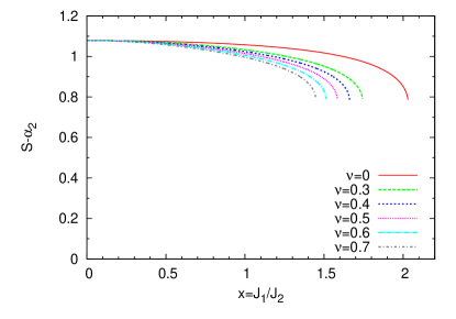
Figure 6: (Color online) Renormalization of the effective exchange parameters by quantum fluctuations as function of $x$ for $S=1$ and $\mu=0.25$. All curves are in the velocity-driven scenario.

Important is the effect of the biquadratic exchange on the renormalization of the quantum correction parameters (for definitions see Eqs. (37, 38, 39)) shown in Fig. 6. The effective exchange perpendicular to the spin stripes is significantly strengthened by factors up to 2, see upper left panel of Fig. 6. In contrast, the effective exchange parallel to the spin stripes stays almost constant except for small frustrations and in vicinity of the end point, see upper right panel of Fig. 6. Because the biquadratic exchange in the Hamiltonian (35) is restricted to in-plane NN sites, the only effect on the renormalization of the interlayer and NNN exchange is the shift of the critical point to smaller values of $x$, see lower panels of Fig. 6. Hence, we indeed find the expected effect that an NN biquadratic exchange enhances the spatial anisotropy. This validates our qualitative considerations in Sect. I.2.

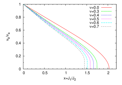
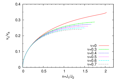
Figure 7: (Color online) Ratios of the spin-wave velocities as a function of $x$ for $S=1$ and $\mu=0.25$. All curves are in the velocity-driven scenario, i.e., the ratio $v_{b}/v_{a}$ vanishes at the end point. This is at the limit of the resolution of the numerical evaluation of the three-dimensional integrals.

The ratios of the spin-wave velocities depicted in Fig. 7 are weakened by increasing biquadratic exchange because the strengthening of the effective exchange perpendicular to the stripes leads to a greater spin-wave velocity $v_{a}$ and thus to a smaller ratio $v_{b}/v_{a}$. In general, the qualitative behavior of the ratios is similar to the one observed without biquadratic exchange.

All in all, a biquadratic exchange acting on in-plane NN sites increases the anisotropy of the exchange parallel and perpendicular to the spin stripes. The growing anisotropy with increasing biquadratic exchange $\nu=J_{\text{bq}}/J_{1}$ is caused by the strong renormalization of the exchange perpendicular to the spin stripes. The exchange parallel to the spin stripes experiences a marginal strengthening and is weakened only in proximity to the critical point. Hence, even a large biquadratic exchange does not induce an effective ferromagnetic exchange $J_{1b}^{\text{eff}}\lessapprox 0$ in $b$-direction.

To render this point quantitatively we define the effective exchange couplings

$$J_{1a}^{\text{eff}} :=J_{2}x_{1a}(1-\alpha_{1}/S)$$ (46a)

$$J_{1b}^{\text{eff}} :=J_{2}x_{1b}(1-\beta/S)$$ (46b)

$$J_{c}^{\text{eff}} :=J_{c}(1-\alpha_{c}/S)$$ (46c)

$$J_{2}^{\text{eff}} :=J_{2}(1-\alpha_{2}/S)$$ (46d)

according to the mean-field Hamiltonians (38b, 38c, 38d, 38e). These definitions enable a direct comparison of the effective spatial anisotropy to the ones determined in fits based on linear spin-wave theory as they are used in experiment Diallo et al. (2009); Zhao et al. (2009), for the analysis of density-functional theory Han et al. (2009) and in other theoretical analyses Schmidt et al. (2010); Yao and Carlson (2010) The relative anisotropy is shown in Fig. 8 for the two-dimensional model, i.e., for $J_{c}=0$. The results for finite three-dimensional coupling are qualitatively the same.

Strikingly, the size of the spin really matters due to the different relative importance of quantum fluctuations. For $S=1$ the self-consistency procedure prevents the occurrence of negative effective couplings in $b$ direction – even for very large biquadratic exchange. This can be understood by inspecting Eq. (39b). For large $\nu$ the expectation value $\beta$ goes to zero. Hence the influence of the square bracket multiplying $\nu$ decreases more and more because the terms independent of $\beta$, i.e., $2S^{3}-2S^{2}$, cancel for $S=1$. Hence no zero or negative effective coupling along the spin stripes occurs. Only for $S>1$ a zero or even negative effective coupling along the direction of parallel spins is possible. We will come back to this point when comparing with experimental data.

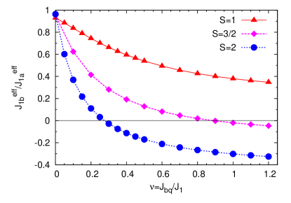
Figure 8: (Color online) Relative anisotropy, cf. definitions (46), as function of the relative biquadratic exchange $\nu$ in the two-dimensional model for $S=1$, $3/2$ and $S=2$.

V Application to the Iron Pnictides

Here we discuss the applicability of our model to iron pnictides. We consider $S=1$, $S=3/2$ and $S=2$. The former value is suggested by the relatively low values for the staggered magnetizations measured de la Cruz et al. (2008); Ewings et al. (2008); Zhao et al. (2008a); McQueeney et al. (2008); Zhao et al. (2009), see also list in Ref. Schmidt et al., 2010. Further support for this value comes from the successful studies of two-band models Raghu et al. (2008); Lee et al. (2010a, b). Another interesting support is provided by advanced Gutzwiller calculations of the distribution of local charges in five-band models which are consistent with $S=1$ Schickling et al. (2011). On the other hand, simple chemical electron count implies that the iron is doubly positive charged so that the d-shell contains four holes and Hund’s rule implies $S=2$. Indeed, recent findings for closely related iron compounds showed that static local moments up to $2.2-3.3\mu_{\text{B}}$ can occur Bao et al. (2011); Li et al. (2011); Pomjakushin et al. (2011) or even larger ($4.7\mu_{\text{B}}$) Ryan et al. (2011). Furthermore, we stress that the value of the staggered static magnetization per site represents only a lower bound for the local moment. Moreover, the observable static moment also depends on electronic matrix elements Uhrig et al. (2009) influenced by the complicated electronic situation. In view of these ambiguities, it is certainly worthwhile to consider also $S=3/2$ and $S=2$.

Experimentally, the magnetic dispersion is best known for the 122 compound CaFe₂As₂ McQueeney et al. (2008); Diallo et al. (2009); Zhao et al. (2009). Hence we fit the dispersion obtained by self-consistent mean-field theory of the three-dimensional model (35) with biquadratic exchange to the measured spin-wave dispersion. Then we are able to draw conclusions regarding the quality of the agreement and the plausibility of the exchange values obtained.

$\nu$	0.3	0.4	0.5	0.6	3.0
$x$	0.645	0.616	0.589	0.565	0.284
$\mu$	0.297	0.314	0.332	0.349	0.793
$J_{1}$	18.9	17.9	16.9	16.0	7.1
$J_{c}$	5.6	5.6	5.6	5.6	5.6
$J_{2}$	29.4	29.0	28.7	28.4	24.9
$J_{\text{bq}}$	5.7	7.1	8.5	9.6	21.2
$J^{\text{eff}}_{1a}$	25.4	26.3	27.1	27.9	36.2
$J^{\text{eff}}_{1b}$	18.8	17.9	17.0	16.3	8.0
$J^{\text{eff}}_{c}$	5.3	5.3	5.3	5.3	5.3
$J^{\text{eff}}_{2}$	31.1	30.7	30.3	29.9	25.8

Table 2: Fit parameters of the model (35) in the three dimensional columnar phase for given values of the relative biquadratic exchange $\nu=J_{\text{bq}}/J_{1}$. The parameters are determined by fits to the experimental spin-wave velocities in CaFe₂As₂ Zhao et al. (2009). The exchange constants $J^{\text{eff}}_{i}$ are the exchange constants which would provide the same results for a model without biquadratic exchange in linear spin-wave theory, see the definitions (46).

The results of fits to Zhao’s data are given in Tab.  2 for plausible values of $J_{\text{bq}}$. In order to fix $J_{\text{bq}}$ independently an additional fourth piece of information is required from experiment, for instance the energy at $k=(0,1,0)$. This energy was only determined by Zhao et al. Zhao et al. (2009). The curves shown in Fig. 9 illustrate that perfect agreement is possible for small energies and perpendicular to the spin stripes, i.e., the direction of parallel spins. We refrain from showing the results for Diallo’s experimental data. The results are very similar, despite the smaller interlayer coupling derived from Diallo’s INS data. The interested reader is referred to Ref. Stanek, 2010.

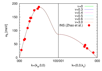
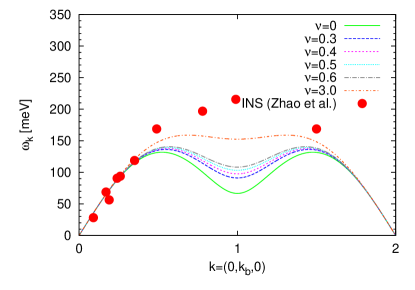
Figure 9: (Color online) Spin-wave dispersion (40) resulting from the self-consistent mean-field theory of the model (35) for $S=1$ in the three dimensional columnar phase with biquadratic exchange for various values of $\nu=J_{\text{bq}}/J_{1}$. The dispersions (lines) are plotted for the parameters given in Tab. 2. The red dots are experimental data extracted from INS for CaFe₂As₂ from Ref. Zhao et al., 2009. Wave vectors are given in units of $\pi$ over lattice constants assuming an orthorhombic crystal. Note that along the path in the BZ shown in the left panel all fits collapse in one curve. Significant differences occur only along the path shown in the right panel.

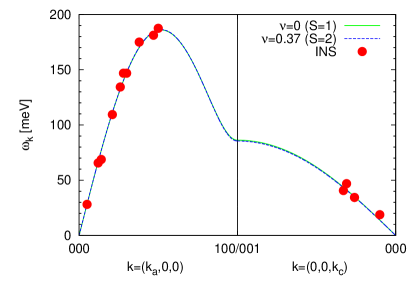
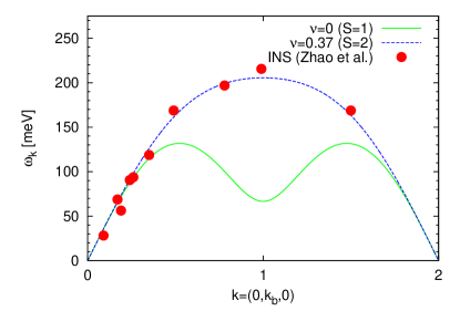
Figure 10: (Color online) Same as in Fig. 9 but for $S=3/2$ and $S=2$, the parameters are given in Tab. 3.

But even for an artificially large biquadratic exchange $\nu=3$ the qualitative behavior of the dispersion along the spin stripes is not described satisfactorily, see right panel of Fig. 9. At first glance, this comes as a surprise since naively a sufficiently large biquadratic exchange should induce an arbitrary spatial anisotropy. But the self-consistency prevents this, see Fig. 8 and Eq. (39b) and the discussion of them.

$S$	$x$	$\mu$	$\nu$	$J_{2}$	$J_{1a}^{\text{eff}}$	$J_{1b}^{\text{eff}}$	$J_{c}^{\text{eff}}$	$J_{2}^{\text{eff}}$
$3/2$	0.52	0.56	1.20	12.4	50.4	-5.7	5.2	18.8
2	0.78	0.37	0.37	9.3	50.4	-5.7	5.2	18.8
Zhao et al.	-	-	-	-	49.9	-5.7	5.3	18.9

Table 3: Fit parameters of the model (35) in the three dimensional columnar phase for $S=3/2$ and $S=2$. The parameters are determined by fits to the experimental dispersions in CaFe₂As₂ Zhao et al. (2009). Exchange couplings in meV. For comparison, the exchange constants $J_{i}^{\text{eff}}$ obtained in linear spin wave theory by Zhao et al. Zhao et al. (2009) are given.

The understanding of the quantitative effect of the biquadratic term tells us that only a larger spin value may lead to the experimentally observed anisotropy. Indeed, for $S=2$ and for $S=3/2$ we achieve a perfect fit, see Tab. 3. But for $S=3/2$ the required value of $J_{\text{bq}}$ appears unreasonably large relative to $J_{1}$. The resulting dispersion is shown in Fig. 10 for $S=2$. The dispersion obtained for $S=3/2$ (not shown) look essentially the same. Note the excellent agreement obtained without assuming any spatial anisotropy in the model itself. It is the magnetic long-range directional Ising-type order which induces the strong spatial anisotropy. We judge the fit parameters necessary for $S=2$ to be perfectly reasonable, in particular the moderate value of the biquadratic exchange of 37%.

The above finding provides an interesting piece of information for the description of the magnetic excitations in the pnictides by a model of localized spins. But it leaves open the issue why the observed staggered moments are much lower than $4\mu_{\text{B}}$ which is the value one would expect for $S=2$. Here we can only speculate that the complicated local electronic levels and the remaining itinerant character of the charges are the physical reasons for this. Also, the issue of line broadening due to Landau damping is not included in the present model Diallo et al. (2009); Knolle et al. (2010); Goswami et al. (2011).

All in all, the additional biquadratic exchange influences the dispersion parallel to the spin stripes and strengthens the anisotropy of the effective in-plane NN exchange constants. However, for $S=1$ it is not possible to reproduce the whole experimental dispersion measured by Zhao et al.. This is possible for $S=3/2$ for parameters which do not appear to be realistic. For $S=2$, the dispersion can be described very well for realistic parameters. The question why the observed magnetic moments are much smaller than one would expect for $S=2$ remains unresolved at present. The local electronic situation and the residual itineracy are likely candidates to reduce the magnetic moment.

VI Dynamic Structure Factor

Besides the dispersion it is the dynamic structure factor $S(\mathbf{k},\omega)$ which matters for the understanding of experimental observations. In addition to the information about the energies of the collective excitations, $S(\mathbf{k},\omega)$ contains information about the relevant matrix elements. In the Dyson-Maleev representation, the inelastic part of the dynamical structure factor for $N$ spins at $T=0$ reads

$$S_{0}^{xx}\left(\mathbf{k},\omega\right) =N\pi\left(S-n\right)\frac{A_{\mathbf{k}}-B_{\mathbf{k}}}{2\sqrt{A_{\mathbf{k}}^{2}-B_{\mathbf{k}}^{2}}}\delta\left(\omega-\omega_{\mathbf{k}}\right),$$ (47)

where $n$, $A_{\mathbf{k}}$ and $B_{\mathbf{k}}$ are defined in Sect. IV. Because of the rotational symmetry about $S^{z}$ , $S^{yy}_{T}(\mathbf{k},\omega)$ is identical to $S^{xx}_{T}(k,\omega)$. In the limit of $\mathbf{k}\rightarrow(0,0,0)$, the dynamical structure factor (47) vanishes because $A_{\mathbf{k}}=B_{\mathbf{k}}$. In the limit of $\mathbf{k}\rightarrow(1,0,1)$, the dynamical structure factor (47) diverges because $A_{\mathbf{k}}=-B_{\mathbf{k}}$. Note that in both cases we have $\omega_{\mathbf{k}}\rightarrow 0$. Similar results have been derived within linear spin-wave theory in Ref. Yao and Carlson, 2010.

Constant-energy cuts are computed from (47) for equally weighted twinned domains. This means that the spatially anisotropic result from (47) is superposed for one choice of the crystallographic $a$ and $b$ directions and for the swapped choice $a\leftrightarrow b$ so that the resulting superposition is spatially isotropic in the sense that there is no difference between the $a$ and the $b$ direction. The results for $S=1$ are shown in Fig. 11; those for $S=2$ in Fig. 12. They are to be compared with the experimental findings in Ref. Zhao et al., 2009.

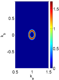
(a) $E=48\pm 6$ meV, $k_{c}=3$

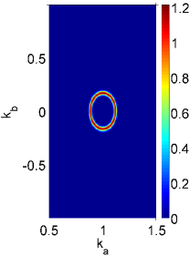
(b) $E=65\pm 4$ meV, $k_{c}=3$

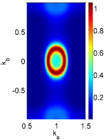
(c) $E=100\pm 10$ meV, $k_{c}=3.5$

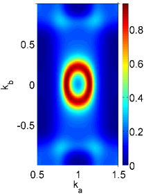
(d) $E=115\pm 10$ meV, $k_{c}=4$

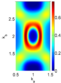
(e) $E=137\pm 15$ meV, $k_{c}=4$

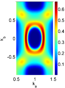
(f) $E=135\pm 10$ meV, $k_{c}=4.5$

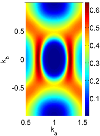
(g) $E=144\pm 15$ meV, $k_{c}=5$

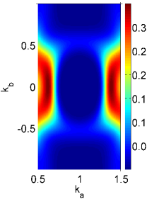
(h) $E=175\pm 15$ meV, $k_{c}=5.2$

Figure 11: (Color online) Constant-energy cuts of the dynamical structure factor per spin (47) integrated over the given energy interval for a twinned sample for $S=1$ and the relative biquadratic exchange $\nu=0.5$. Other parameters are given in Tab. 2. The range of $k_{a,b}$ and the values of $k_{c}$ and $E$ have been chosen to match the rendering of the experimental data Zhao et al. (2009). The reciprocal lattice vectors are given in units $\pi$/lattice constant. Note that the weights in the given energy intervals are dimensionless according to formula (47).

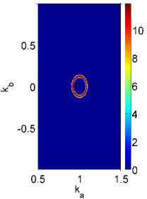
(a) $E=48\pm 6$ meV, $k_{c}=3$

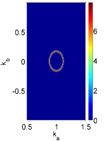
(b) $E=65\pm 4$ meV, $k_{c}=3$

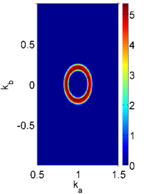
(c) $E=100\pm 10$ meV, $k_{c}=3.5$

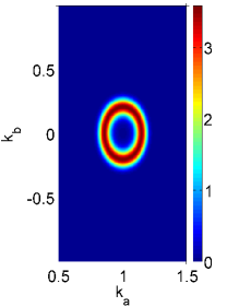
(d) $E=115\pm 10$ meV, $k_{c}=4$

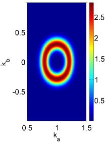
(e) $E=137\pm 15$ meV, $k_{c}=4$

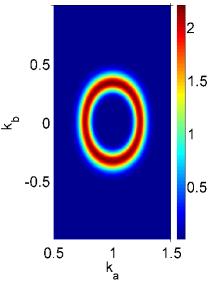
(f) $E=135\pm 10$ meV, $k_{c}=4.5$

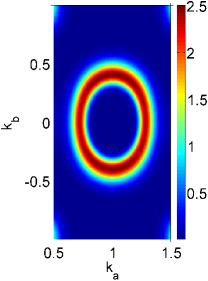
(g) $E=144\pm 15$ meV, $k_{c}=5$

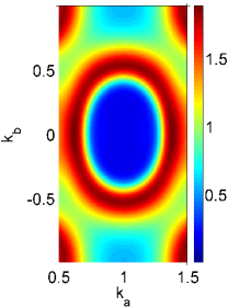
(h) $E=175\pm 15$ meV, $k_{c}=5.2$

Figure 12: Same as in the previous Fig. 11, but for $S=2$. The parameters are given in Tab. 3.

For low energies, concentric rings emerge from the magnetic ordering vector $Q=(1,0,3)$. They display a certain ellipticity which is not surprising in view of the spatial anisotropy of the spin order. The rings increase in size for higher energies. For $S=1$ (Fig. 11), less intensive spots $(1,1,k_{c})$ appear additionally for $E=100$ meV and $E=115$ meV which merge with the concentric spin-wave rings for higher energies. For $S=2$ (Fig. 12), the circular signatures of the dispersion cones persist up to 144meV; only for even higher energies significant additional features occur. In general, one observes the trend of decreasing intensity for increasing energy because $S(\mathbf{k},\omega)\propto 1/\omega_{\mathbf{k}}$, see Eq. (47).

The comparison to the experimental data Zhao et al. (2009) shows that the $S=2$ results match better which is not surprising since they reproduce the dispersion everywhere, see Fig. 10. The experimental data displays also rings of high scattering intensities which increase very much like the theoretical results do. But the experimental results are broader indicating a finite life-time of the magnetic excitations. This effect is lacking in our model for two reasons: (i) The spin-only model does not include any Landau damping due to the decay of magnons into electronic particle-hole pairs. The consideration of this effect would require to pass to a doped $t$-$J$ type of model or to switch completely to an itinerant approach, see for instance Ref. Knolle et al., 2010. (ii) Even in the framework of a spin-only model the scattering of magnons from other magnons will lead to life-time effects which are not taken into account by a mean-field approach.

Hence, the agreement of Fig. 12 to the experimental data is encouraging, in particular in view of the neglect of damping effects. We conclude that the description of the magnetic excitations of undoped pnictides within a model of localized spins is possible if a significant biquadratic exchange is included and $S=2$ is chosen.

VII Conclusions

In this paper, we obtained the following results:
First, we pointed out that the instability of the columnar phase, i.e., the phase with spin stripes, can become unstable in two qualitatively different ways in three dimensions. Either the sublattice magnetization vanishes so that the long-range order parameter vanishes (magnetization-driven scenario). Or the smallest spin-wave velocity vanishes (velocity-driven scenario). The latter scenario is not possible in two dimensions because a vanishing velocity implies a logarithmically diverging correction of the quantum corrections of the magnetization so that the magnetization will always vanish before the velocity becomes zero. But the subtlety of a logarithmic divergence makes it numerically difficult to detect the vanishing magnetization, in particular for large values of the spin. We presume that the magnetization-driven scenario leads to a weak first order transition to a possible intermediate phase and that the velocity-driven scenario indicates a strong first order transition to the Néel phase.

Second, we discussed the importance of a biquadratic exchange. The motivation is the very distinctive spatial anisotropy of the dispersion in the pnictides which cannot be induced by the small distortive anisotropy. In order to be able to treat biquadratic exchange on the same footing as we treated nearest-neighbor Heisenberg Hamiltonians before we studied two mean-field approaches to biquadratic exchange. One is based on the Dyson-Maleev representation, the other on the Schwinger boson representation. Surprisingly, even at zero temperature these mean-field theories provide distinctively different results. We tested both approaches for the Néel phase of the nearest-neighbor Heisenberg on the square lattice against series expansion data and exact diagonalization. We established that the Dyson-Maleev mean-field theory provides reliable results within about 10% of the contribution of the biquadratic exchange.

Third, we applied the developed mean-field approach to the columnar phase of the $J_{1}$-$J_{\text{bq}}$-$J_{2}$-$J_{c}$ Heisenberg model in three dimensions. The aim was to explain the magnetic dispersions observed in the undoped iron pnictides, parent compounds of a novel class of superconductors. It turned out that a biquadratic exchange indeed enhances the spatial anisotropy of the spin-wave velocities. But the effect is reduced by quantum corrections so that it is not large enough for $S=1$ to match the experimental situation. Only for larger values of $S$ an almost vanishing effective coupling in $b$ direction along the stripes of parallel spins is possible. For $S=3/2$, however, the required exchange couplings are unlikely. For instance, the biquadratic exchange would have to be larger than the nearest neighbor exchange. But for $S=2$ perfect agreement of the dispersion is obtained without invoking any spatial anisotropy of the model itself. Note that $S=2$ corresponds to the chemical valence Fe²⁺ which follows from an ionic balance of charge in the pnictides. This valence implies four holes in the d-shell so that the maximum spin according to Hund’s rule is $S=2$. We provided also results for the dynamic structure factor for the matching model at $S=2$ and for $S=1$ for comparison.

Of course, there are open points which are beyond the scope of the present article. First, there is the relatively small staggered moments seen in experiment which indicate rather smaller than larger spin values. The complicated local electronic situation and the residual itineracy of the charges are likely candidates to cause this discrepancy. But we mention that recent experiments also found large moments in related substances which are also superconducting. Second, the spin-only model considered here does not include the important charge degrees of freedom which generate Landau damping and the bad metallic behavior of the externally undoped parent pnictides. So life-time effects are not treated.

Further research is called for: On the level of localized spin models the investigation of the recently found high-spin substances appears to be interesting but may require the more challenging treatment of canted magnetic order. On the level of itinerant charges the influence of doped charges has to be studied. These charges can be externally doped or internally self-doped between the bands. Furthermore, it would be interesting to learn more about the values for biquadratic exchanges from density-functional calculations.

Appendix A Dyson-Maleev representation

A.1 Antiferromagnetic exchange

For antiparallel orientation of coupled spins, the Hamiltonian (5) is given in Dyson-Maleev representation by

$$H^{\text{afm}} =H_{\text{bl}}^{\text{afm}}+H_{\text{bq}}^{\text{afm}},$$ (48)

with

$$H^{\text{afm}}_{\text{bl}} =J\sum\limits_{\langle i,j\rangle}\biggl{\{}-S^{2}+S\left(\hat{n}_{i}+\hat{n}_{j}+b^{\dagger}_{i}b^{\dagger}_{j}+b^{\phantom{\dagger}}_{i}b^{\phantom{\dagger}}_{j}\right)-\hat{n}_{i}\hat{n}_{j}-\frac{1}{2}\left(b^{\dagger}_{i}\hat{n}_{i}b^{\dagger}_{j}+b^{\phantom{\dagger}}_{i}\hat{n}_{j}b^{\phantom{\dagger}}_{j}\right)\biggr{\}}$$ (49a)

$$\begin{split}H^{\text{afm}}_{\text{bq}}&=-J_{\text{bq}}\sum\limits_{\langle i,j\rangle}\biggl{\{}S^{4}-2S^{3}\left(\hat{n}_{i}+\hat{n}_{j}+\hat{I}_{0}\right)\biggr{.}\\ &\quad+S^{2}\left[\hat{n}^{2}_{i}+\hat{n}_{j}^{2}+4\hat{n}_{i}\hat{n}_{j}+\hat{I}^{2}_{0}+\left(\hat{n}_{i}+\hat{n}_{j}\right)\hat{I}_{0}+\hat{I}_{0}\left(\hat{n}_{i}+\hat{n}_{j}\right)+\hat{I}^{\prime}_{0}\right]\\ &\quad-S\left[2\left(\hat{n}_{i}\hat{n}_{j}^{2}+\hat{n}_{i}^{2}\hat{n}_{j}\right)+\hat{n}_{i}\hat{n}_{j}\hat{I}_{0}+\hat{I}_{0}\hat{n}_{i}\hat{n}_{j}+\frac{1}{2}\bigl{(}\hat{I}^{\phantom{\dagger}}_{0}\hat{I}^{\prime}_{0}+\hat{I}^{\prime}_{0}\hat{I}_{0}^{\phantom{\dagger}}+\left(\hat{n}_{i}+\hat{n}_{j}\right)\hat{I}^{\prime}_{0}+\hat{I}_{0}^{\prime}\left(\hat{n}_{i}+\hat{n}_{j}\right)\bigr{)}\right]\\ &\biggl{.}\quad+\hat{n}_{i}^{2}\hat{n}_{j}^{2}+\frac{1}{4}\hat{I}_{0}^{\prime 2}+\frac{1}{2}\left(\hat{n}_{i}\hat{n}_{j}\hat{I}_{0}^{\prime}+\hat{I}_{0}^{\prime}\hat{n}_{i}\hat{n}_{j}\right)\biggr{\}}\end{split}$$ (49b)

where

$$\hat{I}_{0} :=b^{\dagger}_{i}b^{\dagger}_{j}+b^{\phantom{\dagger}}_{i}b^{\phantom{\dagger}}_{j}$$ (50a)

$$\hat{I}_{0}^{\prime} :=b^{\dagger}_{i}\hat{n}_{i}^{\phantom{\dagger}}b^{\dagger}_{j}+b_{i}^{\phantom{\dagger}}\hat{n}_{j}^{\phantom{\dagger}}b_{j}^{\phantom{\dagger}}$$ (50b)

with $i,j$ being the two coupled sites. For the mean-field decoupling the reader is referred to Eq. (38).

A.2 Ferromagnetic exchange

For parallel orientation of coupled spins, the Hamiltonian (5) in Dyson-Maleev representation reads

$$H^{\text{fm}} =H_{\text{bl}}^{\text{fm}}+H_{\text{bq}}^{\text{fm}}$$ (51)

where

$$H_{\text{bl}}^{\text{fm}} =J\sum\limits_{\langle i,j\rangle}\left\{S^{2}-S\left(\hat{n}_{i}^{\phantom{\dagger}}+\hat{n}_{j}^{\phantom{\dagger}}-b^{\dagger}_{i}b^{\phantom{\dagger}}_{j}-b^{\dagger}_{j}b^{\phantom{\dagger}}_{i}\right)+\hat{n}_{i}^{\phantom{\dagger}}\hat{n}_{j}^{\phantom{\dagger}}-\frac{1}{2}\left(b^{\dagger}_{i}\hat{n}_{i}^{\phantom{\dagger}}b^{\phantom{\dagger}}_{j}+b^{\dagger}_{j}\hat{n}_{j}^{\phantom{\dagger}}b^{\phantom{\dagger}}_{i}\right)\right\}$$ (52a)

$$\begin{split}H_{\text{bq}}^{\text{fm}}&=-J_{\text{bq}}\sum\limits_{\langle i,j\rangle}\biggl{\{}S^{4}-2S^{3}\left(\hat{n}_{i}+\hat{n}_{j}-\hat{F}_{0}\right)\biggr{.}\\ &\quad+S^{2}\left[\hat{n}_{i}^{2}+\hat{n}_{j}^{2}+4\hat{n}_{i}\hat{n}_{j}+\hat{F}^{2}_{0}-\left(\hat{n}_{i}+\hat{n}_{j}\right)\hat{F}_{0}-\hat{F}_{0}\left(\hat{n}_{i}+\hat{n}_{j}\right)-\hat{F}^{\prime}_{0}\right]\\ &\quad+S\left[-2\left(\hat{n}_{i}\hat{n}_{j}^{2}+\hat{n}_{i}^{2}\hat{n}_{j}\right)+\hat{n}_{i}\hat{n}_{j}\hat{F}_{0}+\hat{F}_{0}\hat{n}_{i}\hat{n}_{j}+\frac{1}{2}\bigl{(}-\hat{F}^{\phantom{\dagger}}_{0}\hat{F}_{0}^{\prime}-\hat{F}_{0}^{\prime}\hat{F}^{\phantom{\dagger}}_{0}+\left(\hat{n}_{i}+\hat{n}_{j}\right)\hat{F}_{0}^{\prime}+\hat{F}_{0}^{\prime}\left(\hat{n}_{i}+\hat{n}_{j}\right)\bigr{)}\right]\\ &\quad\biggl{.}+\hat{n}^{2}_{i}\hat{n}_{j}^{2}+\frac{1}{4}\hat{F}_{0}^{\prime 2}-\frac{1}{2}\left(\hat{n}^{\phantom{\dagger}}_{i}\hat{n}^{\phantom{\dagger}}_{j}\hat{F}^{\prime}_{0}+\hat{F}^{\prime}_{0}\hat{n}^{\phantom{\dagger}}_{i}\hat{n}^{\phantom{\dagger}}_{j}\right)\biggr{\}}\end{split}$$ (52b)

with

$$\hat{F}_{0} :=b^{\dagger}_{i}b^{\phantom{\dagger}}_{j}+b^{\dagger}_{j}b^{\phantom{\dagger}}_{i}$$ (53a)

$$\hat{F}^{\prime}_{0} :=b^{\dagger}_{i}\hat{n}_{i}^{\phantom{\dagger}}b^{\phantom{\dagger}}_{j}+b^{\dagger}_{j}\hat{n}_{j}^{\phantom{\dagger}}b^{\phantom{\dagger}}_{i}.$$ (53b)

For the mean-field decoupling the reader is referred to Eq. (38).

References

- Lacroix et al. (2011) C. Lacroix, P. Mendels, and F. Mila, eds., Introduction to Frustrated Magnetism, vol. 164 of Springer Series in Solid-State Sciences (Springer, Berlin, 2011).
- Xu and Ting (1990) J. H. Xu and C. S. Ting, Phys. Rev. B 42, 6861 (1990).
- Irkhin et al. (1992) V. Y. Irkhin, A. A. Katanin, and M. I. Katsnelson, J. Phys.: Condens. Mattter 4, 5227 (1992).
- Singh et al. (1999) R. R. P. Singh, Z. Weihong, C. J. Hamer, and J. Oitmaa, Phys. Rev. B 60, 7278 (1999).
- Kotov et al. (1999) V. N. Kotov, J. Oitmaa, O. P. Sushkov, and W. Zheng, Phys. Rev. B 60, 14613 (1999).
- Sushkov et al. (2001) O. P. Sushkov, J. Oitmaa, and Z. Weihong, Phys. Rev. B 63, 104420 (2001).
- Singh et al. (2003) R. R. P. Singh, W. Zheng, J. Oitmaa, O. P. Sushkov, and C. J. Hamer, Phys. Rev. Lett. 91, 017201 (2003).
- Bishop et al. (2008) R. F. Bishop, P. H. Y. Li, R. Darradi, and J. Richter, Europhys. Lett. 83, 47004 (2008).
- Uhrig et al. (2009) G. S. Uhrig, M. Holt, J. Oitmaa, O. P. Sushkov, and R. R. P. Singh, Phys. Rev. B 79, 092416 (2009).
- Majumdar (2010) K. Majumdar, Phys. Rev. B 82, 144407 (2010).
- Schmalfuß et al. (2006) D. Schmalfuß, R. Darradi, J. Richter, J. Schulenburg, and D. Ihle, Phys. Rev. Lett. 97, 157201 (2006).
- Yao and Carlson (2010) D.-X. Yao and E. W. Carlson, Front. Phys. China 5, 166 (2010), eprint 0910.2528v1.
- Majumdar (2011a) K. Majumdar, J. Phys.: Condens. Mattter 23, 046001 (2011a).
- Majumdar (2011b) K. Majumdar, J. Phys.: Condens. Mattter 23, 116004 (2011b).
- Holt et al. (2011) M. Holt, O. P. Sushkov, D. Stanek, and G. S. Uhrig, Phys. Rev. B 83, 144528 (2011).
- Betts and Oitmaa (1977) D. D. Betts and J. Oitmaa, Phys. Lett. 62A, 277 (1977).
- Manousakis (1991) E. Manousakis, Rev. Mod. Phys. 63, 1 (1991).
- Auerbach (1994) A. Auerbach, Interacting Electrons and Quantum Magnetism, Graduate Texts in Contemporary Physics (Springer, New York, 1994).
- Chandra and Doucot (1988) P. Chandra and B. Doucot, Phys. Rev. B 38, 9335 (1988).
- Yao and Carlson (2008) D.-X. Yao and E. W. Carlson, Phys. Rev. B 78, 052507 (2008).
- Applegate et al. (2010) R. Applegate, J. Oitmaa, and R. R. P. Singh, Phys. Rev. B 81, 024505 (2010).
- Schmidt et al. (2010) B. Schmidt, M. Siahatgar, and P. Thalmeier, Phys. Rev. B 81, 165101 (2010).
- Smerald and Shannon (2010) A. Smerald and N. Shannon, Europhys. Lett. 92, 47005 (2010).
- Chandra et al. (1990) P. Chandra, P. Coleman, and A. I. Larkin, Phys. Rev. Lett. 64, 88 (1990).
- Mermin and Wagner (1966) N. D. Mermin and H. Wagner, Phys. Rev. Lett. 17, 1133 (1966).
- Weber et al. (2003) C. Weber, L. Capriotti, G. Misguich, F. Becca, M. Elhajal, and F. Mila, Phys. Rev. Lett. 91, 177202 (2003).
- Capriotti et al. (2004) L. Capriotti, A. Fubini, T. Roscilde, and V. Tognetti, Phys. Rev. Lett. 92, 157202 (2004).
- Xu et al. (2008) C. Xu, M. Müller, and S. Sachdev, Phys. Rev. B 78, 020501(R) (2008).
- Shannon et al. (2006) N. Shannon, T. Momoi, and P. Sindzingre, Phys. Rev. Lett. 96, 027213 (2006).
- Kamihara et al. (2008) Y. Kamihara, T. Watanabe, M. Hirano, and H. Hosono, J. Am. Chem. Soc. 130, 3296 (2008).
- de la Cruz et al. (2008) C. de la Cruz, Q. Huang, J. W. Lynn, J. Li, W. Ratcliff II, J. L. Zarestky, H. A. Mook, G. F. Chen, J. L. Luo, N. L. Wang, et al., Nature 453, 899 (2008).
- Diallo et al. (2009) S. O. Diallo, V. P. Antropov, T. G. Perring, C. Broholm, J. J. Pulikkotil, N. Ni, S. L. Bud’ko, P. C. Canfield, A. Kreyssig, A. I. Goldman, et al., Phys. Rev. Lett. 102, 187206 (2009).
- Zhao et al. (2009) J. Zhao, D. T. Adroja, D.-X. Yao, R. Bewley, S. Li, X. F. Wang, G. Wu, X. H. Chen, J. Hu, and P. Dai, Nat. Phys. 5, 555 (2009).
- Ren et al. (2008) Z. A. Ren, G.-C. Che, X.-L. Dong, J. Yang, W. Lu, W. Yi, X.-L. Shen, Z.-C. Li, L.-L. Sun, F. Zhou, et al., Europhys. Lett. 83, 17002 (2008).
- Yin et al. (2008) Z. P. Yin, S. Lebègue, M. J. Han, B. P. Neal, S. Y. Savrasov, and W. E. Pickett, Phys. Rev. Lett. 101, 047001 (2008).
- Ewings et al. (2008) R. A. Ewings, T. G. Perring, R. I. Bewley, T. Guidi, M. J. Pitcher, D. R. Parker, S. J. Clarke, and A. T. Boothroyd, Phys. Rev. B 78, 220501 (2008).
- Zhao et al. (2008a) J. Zhao, W. Ratcliff II, J. W. Lynn, G. F. Chen, J. L. Luo, N. L. Wang, J. Hu, and P. Dai, Phys. Rev. B 78, 140504 (2008a).
- McQueeney et al. (2008) R. J. McQueeney, S. O. Diallo, V. P. Antropov, G. D. Samolyuk, C. Broholm, N. Ni, S. Nandi, M. Yethiraj, J. L. Zarestky, J. J. Pulikkotil, et al., Phys. Rev. Lett. 101, 227205 (2008).
- Si and Abrahams (2008) Q. Si and E. Abrahams, Phys. Rev. Lett. 101, 076401 (2008).
- Ong et al. (2009) A. Ong, G. S. Uhrig, and O. P. Sushkov, Phys. Rev. B 80, 014514 (2009).
- Yildirim (2008) T. Yildirim, Phys. Rev. Lett. 101, 057010 (2008).
- Wu et al. (2008) J. Wu, P. Phillips, and A. H. C. Neto, Phys. Rev. Lett. 101, 126401 (2008).
- Lv et al. (2010) W. Lv, F. Krüger, and P. Phillips, Phys. Rev. B 82, 045125 (2010).
- Pulikkotil et al. (2010) J. J. Pulikkotil, L. Ke, M. van Schilfgaarde, T. Kotani, and V. P. Antropov, Supercond. Sci. Technol. 23, 054012 (2010).
- Zhao et al. (2008b) J. Zhao, D.-X. Yao, S. Li, T. Hong, Y. Chen, S. Chang, W. Ratcliff II, J. W. Lynn, H. A. Mook, G. F. Chen, et al., Phys. Rev. Lett. 101, 167203 (2008b).
- Han et al. (2009) M. J. Han, Q. Yin, W. E. Pickett, and S. Y. Savrasov, Phys. Rev. Lett. 102, 107003 (2009).
- Singh (2009) R. R. P. Singh, arXiv:0903.4408 (2009).
- Girardeau and Popovic-Boziv (1977) M. D. Girardeau and M. Popovic-Boziv, J. Phys. C 10, 2471 (1977).
- Mila and Zhang (2000) F. Mila and F.-C. Zhang, Eur. Phys. J. B 16, 7 (2000).
- Hamerla et al. (2010) S. A. Hamerla, S. Duffe, and G. S. Uhrig, Phys. Rev. B 82, 235117 (2010).
- Yaresko et al. (2009) A. N. Yaresko, G.-Q. Liu, V. N. Antonov, and O. K. Andersen, Phys. Rev. B 79, 144421 (2009).
- Graser et al. (2010) S. Graser, A. F. Kemper, T. A. Maier, H.-P. Cheng, P. J. Hirschfeld, and D. J. Scalapino, Phys. Rev. B 81, 214503 (2010).
- Schickling et al. (2011) T. Schickling, F. Gebhard, and J. Bünemann, Phys. Rev. Lett. 106, 146402 (2011).
- Dyson (1956a) F. J. Dyson, Phys. Rev. 102, 1217 (1956a).
- Dyson (1956b) F. J. Dyson, Phys. Rev. 102, 1230 (1956b).
- Maleev (1958) S. Maleev, Sov. Phys. JETP 6, 776 (1958).
- Fetter and Walecka (1971) A. L. Fetter and J. D. Walecka, Quantum Theory of Many-Particle Systems, International Series in Pure and Applied Physics (McGraw-Hill, New York, 1971).
- Lange (1966) R. V. Lange, Phys. Rev. 146, 301 (1966).
- Auerbach and Arovas (1988) A. Auerbach and D. P. Arovas, Phys. Rev. Lett. 61, 617 (1988).
- Arovas and Auerbach (1988) D. P. Arovas and A. Auerbach, Phys. Rev. B 38, 316 (1988).
- Raas (2009) C. Raas, Private communication (2009).
- Oitmaa et al. (2006) J. Oitmaa, C. J. Hamer, and W. Zheng, Series Expansion Methods for Strongly Interacting Lattice Models (Cambridge Univ. Press, Cambridge, 2006).
- Oitmaa (2009) J. Oitmaa, Private communication (2009).
- Stanek (2010) D. Stanek, Diploma thesis, TU Dortmund (2010), URL http://t1.physik.tu-dortmund.de/uhrig/diploma.html.
- Raghu et al. (2008) S. Raghu, X.-L. Qi, C.-X. Liu, D. J. Scalapino, and S.-C. Zhang, Phys. Rev. B 77, 220503 (2008).
- Lee et al. (2010a) H. Lee, Y.-Z. Zhang, H. O. Jeschke, R. Valentí, and H. Monien, Phys. Rev. Lett. 104, 026402 (2010a).
- Lee et al. (2010b) H. Lee, Y.-Z. Zhang, H. O. Jeschke, and R. Valentí, Phys. Rev. B 81, 220506 (2010b).
- Bao et al. (2011) W. Bao, Q. Huang, G. F. Chen, M. A. Green, D. M. Wang, J. B. He, X. Q. Wang, and Y. Qiu, 1102.0830 (2011).
- Li et al. (2011) Z. Li, X. Ma, H. Pang, and F. Li, p. 1103.0098 (2011).
- Pomjakushin et al. (2011) V. Y. Pomjakushin, E. V. Pomjakushina, A. Krzton-Maziopa, K. Conder, and Z. Shermadini, p. 1102.3380 (2011).
- Ryan et al. (2011) D. Ryan, W. Rowan-Weetaluktuk, J. Cadogan, R. Hu, W. Straszheim, S. Bud ko, and P. Canfield, p. 1103.0059 (2011).
- Knolle et al. (2010) J. Knolle, I. Eremin, A. V. Chubukov, and R. Moessner, Phys. Rev. B 81, 140506(R) (2010).
- Goswami et al. (2011) P. Goswami, R. Yu, Q. Si, and E. Abrahams, p. 1009.1111 (2011).