Writing electronic ferromagnetic states in a high-temperature paramagnetic nuclear spin system

Abstract

In this paper we use the Nuclear Magnetic Resonance (NMR) to write eletronic states of a ferromagnetic system into a high-temperature paramagnetic nuclear spins. Through the control of phase and duration of radiofrequency pulses we set the NMR density matrix populations, and apply the technique of quantum state tomography to experimentally obtain the matrix elements of the system, from which we calculate the temperature dependence of magnetization for different magnetic fields. The effects of the variation of temperature and magnetic field over the populations can be mapped in the angles of spins rotations, carried out by the RF pulses. The experimental results are compared to the Brillouin functions of ferromagnetic ordered systems in the mean field approximation for two cases: the mean field is given by (i) $B=B_{0}+\lambda M$ and (ii) $B=B_{0}+\lambda M+\lambda^{\prime}M^{3}$, where $B_{0}$ is the external magnetic field, and $\lambda,\lambda^{\prime}$ are mean field parameters. The first case exhibits second order transition, whereas the second case has first order transition with temperature hysteresis. The NMR simulations are in good agreement with the magnetic predictions.

I Introduction

Magnetism and magnetic materials are among the main branches of research in modern Condensed Matter Physics. Magnetic materials have been extensively studied for decades by a variety of experimental techniques, including Nuclear Magnetic Resonance (NMR) livro_apg . In a standard NMR experiment, a sequence of radiofrequency (RF) pulses is applied to a sample, which may or may not be subject to a static external magnetic field (for the last case, zero-field NMR). Typical information obtained in such NMR experiments are: local magnetic fields and moments, spin and charge distributions, magnetic anisotropy, relaxation dynamics, etc. For reviews of NMR on magnetic materials see Ref. livro_apg and references therein.

For the last ten years NMR has been established also as an useful tool for Quantum Information Processing (QIP), and several quantum algorithms and protocols have been tested in the period. The reason for this is the fact that RF pulses are equivalent to unitary transformations, which are needed for QIP, and can be controlled with great precision in NMR experiments, allowing the manipulation of the quantum states of a system 2005_JChemPhys_122_041101 ; 2006_PRL_96_170501 and generation of protocols to process quantum information 2000_ForPhysik_48_875 ; livro_NMRivan ; 1998_Nature_396_52 . Particularly interesting is the use of NMR–QIP to simulate quantum systems 2004_JMR_166_147 ; 2005_PRA_71_012307 ; 2007_NJP_10_033020 ; 2008_PRL_101_120503 ; 2009_JChemPhys_Accepted .

In an usual quantum simulation performed by NMR, the quantum dynamics of a given system is emulated by mapping the Hamiltonian of the system into the NMR Hamiltonian 2005_PRA_71_012307 ; 1999_PRL_82_5381 ; 2001_PRA_64_032306 ; 2005_PRA_71_032344 ; 2006_ChemPhysLett_422_20 . In this work, we use NMR to write electronic states of a ferromagnetic ordered material into the paramagnetic nuclei density matrix. This is made by first calculating the trace distance between the respective density matrices for various temperatures, and then working out the pulse sequences to achieve the correct eletronic state. The results show how well nuclear states can be used as a quantum memory and, although the present study does not exploit the influence over the eletronic magnetization curve, it is our belief that such studies could bring to NMR a new useful way to study the magnetization dynamics of materials. Some possible applications are discussed on the conclusions.

II Mean-field model of magnetic systems

Magnetic systems are usually modeled using the Heisenberg Hamiltonian which, in the mean-field approximation, can be simplified to livro_apg :

$$\mathcal{H}=-g\,\mu_{B}\,{\bf B}\cdot{\bf S}\,,$$ (1)

and the electronic magnetization is given by (for the $z$-component of spins):

$$M=g\,\mu_{B}{\rm tr}[\rho(T)S_{z}]=g\,\mu_{B}\,S\,\mathcal{B}_{S}(x)\,,$$ (2)

where $\rho(T)$ stands for the thermal equilibrium density matrix, $x=g\mu_{B}\,B\,S/k_{B}T$ and $\mathcal{B}_{S}(x)$ is the Brillouin function. In a paramagnetic isolated spin system, the field $B$ is just the external field $B_{0}$. In the mean field approximation, on the other hand, exchange interaction is parameterized by an effective field $B=B_{0}+\lambda M$, where $\lambda=2(g-1)^{2}zJ_{ex}/g^{2}\mu_{B}^{2}$ is called ‘mean-field parameter’, $g$ is the Landé $g-$factor, $z$ the number of first neighbors, $\mu_{B}$ the Bohr magneton, $J_{ex}$ the exchange parameter and Eq.(2) must be solved self-consistently livro_apg . One of the main aspects of the mean-field approximation is that it predicts magnetic ordering below a critical temperature $T_{c}=g^{2}\mu_{B}^{2}\,S\,(S+1)\,\lambda/3\,k_{B}$. From this relation we can observe that the critical temperature gives us a measure of the exchange parameter $\lambda$.

In particular, the Brillouin function for a spin $S=3/2$ is given by:

$$\mathcal{B}_{3/2}(x)=\frac{2}{3}\left\{2\,\coth\left(2\,x\right)-\frac{1}{2}\coth\left(\frac{x}{2}\right)\right\}.$$ (3)

Equations (2) and (3) will be used to compare the mean-field prediction for an ordered magnetic system with the NMR results of ²³Na in a room temperature liquid-crystal sample.

III NMR two qubit systems

A nuclear system composed by two interacting nuclei, $A$ and $B$, with $I=1/2$ spins in a static magnetic field is the prototype of a two-qubit NMR quantum computer 2000_ForPhysik_48_875 ; 2001_ProgNMRSpec_38_325 ; 2004_RMP_76_1037 ; livro_NMRivan ; livro_suter . The Hamiltonian of such a system is:

$$\mathcal{H}_{1/2,1/2}=-\hbar\omega_{L_{A}}I_{z,A}-\hbar\omega_{L_{B}}I_{z,B}+2\pi J\,I_{z,A}\,I_{z,B}\,,$$ (4)

where $\omega_{L_{A(B)}}$ are the respective Larmor frequencies, and $2\pi J$ is the coupling constant. Such a Hamiltonian describes a four-level system, for instance, coupled ¹H and ¹³C spins in a molecule of Chloroform, under a static magnetic field. Alternatively, a four-level system can be described by a NMR system composed by a spin 3/2 nucleus in a static magnetic field and in the presence of a local electric field gradient. In such case, the Hamiltonian is given by livro_apg :

$$\mathcal{H}_{3/2}=-\hbar\omega_{L}I_{z}+\frac{\hbar\omega_{Q}}{6}\left(3{I}_{z}^{2}-{I}^{2}\right)\,,$$ (5)

where $\omega_{Q}$ is the quadrupole coupling constant. This system can be used to emulate any two-qubit quantum system 2003_PRA_68_032304 ; 2000_JChemPhys_112_6963 ; 2002_QIP_1_327 ; 2005_JMagRes_175_226 ; 2008_JMagRes_192_17 . In NMR systems the Zeeman energy levels are very small if compared to the thermal energy at room temperature. This means that at room temperature the NMR density matrix can be written as livro_ernst ; livro_abragam ; livro_NMRivan ; 2008_JChemPhys_128_052206 :

$$\rho=\frac{1}{2^{n}}\mathbb{I}+\epsilon\Delta\rho\,,$$ (6)

where $\mathbb{I}$ is the $2^{n}\times 2^{n}$ identity matrix, $n$ is the number of qubits, $\Delta\rho=I_{z}$ is the deviation density matrix and $\epsilon=\hbar\omega_{L}/2^{n}k_{B}T\sim 10^{-5}$.

Unfortunately, such state given in Eq.(6) is inadequate for quantum computing proposes, since for that it is necessary a pure inicial state livro_NMRivan . However, the NMR ability for manipulating spins states resulted in a method for creating states isomophic to a pure state, named pseudo-pure states 1997_Science_275_350 ; 1997_PNAS_94_1634 . Such pseudo-pure states (PPS), typically have the form:

$$\rho=\frac{(1-\epsilon)}{2^{n}}\mathbb{I}+\epsilon\,\rho_{1}\,.$$ (7)

There are some different methods to create these states livro_NMRivan . In this work we have used the time-averaging method; the basic pulse sequences for generating pseudopure states in a $I=3/2$ quadrupole system are given in Refs.2003_PRA_68_022311 ; 2002_PRA_66_042310 ; 2001_JChemPhys_114_4415 .

Upon the application of a sequence of radio-frequency pulses representing an unitary transformation, $U$, Eq.(7) transform accordingly:

$$U\rho U^{{\dagger}}=\frac{(1-\epsilon)}{2^{n}}\,\mathbb{I}+\epsilon U\rho_{1}U^{{\dagger}}\,.$$ (8)

From the application of a sequence of such pulses, by setting the pulses duration, phase and amplitude, a very fine control over the density matrix population and coherences can be achieved, and it is possible to generate all two-qubit computational base states, also superposition and entangled states 2005_JMagRes_175_226 ; 2003_PRA_68_022311 . It is important to note that these entangled states are called pseudo-entangled states because $\epsilon\sim 10^{-5}$, which makes $\rho_{pps}$ always separable even when $\rho_{1}$ is an entagled state 1999_PRL_83_1054 .

IV Writting ferromagnetic states into NMR states

Equation (2) can be used to write ferromagnetic electronic states into a high-temperature paramagnetic nuclear spin system. As a prototype we consider a coupled two-spin $I=1/2$ system. The initial state $\rho_{1}$ corresponds to the pseudo-pure state 2003_PRA_68_022311 ; 2005_JMagRes_175_226 $|00\rangle\langle 00|$. The sates are labeled as $|00\rangle,|01\rangle,|10\rangle$, and $|11\rangle$, for increasing order of energy, in accordance to the current literature of NMR quantum information, where each spin $1/2$ represents a qubit.

Considering rotation angles $\theta_{j}^{A}$ and $\theta_{j}^{B}$, of the two spins ($A$ and $B$) over the directions $x$ and $y$ by the operator $R_{x,y}(\theta_{x}^{A},\theta_{x}^{B},\theta_{y}^{A},\theta_{y}^{B})=R_{x}(\theta_{x}^{A})\,R_{x}(\theta_{x}^{B})\,R_{y}(\theta_{y}^{A})\,R_{y}(\theta_{y}^{B})$, where the rotation matrices are given by:

$$R_{j}(\theta_{j}^{A})=\mathbb{I}^{A}\otimes\mathbb{I}^{B}\cos\theta_{j}^{A}-i\,I_{j}^{A}\otimes\mathbb{I}^{B}\sin\theta_{j}^{A},$$ (9)

$$R_{j}(\theta_{j}^{B})=\mathbb{I}^{A}\otimes\mathbb{I}^{B}\cos\theta_{j}^{B}-i\,\mathbb{I}^{A}\otimes I_{j}^{B}\sin\theta_{j}^{B},$$ (10)

and $j=x,y$, we arrive at the following populations:

$$\begin{array}[]{c}\rho_{00}=\frac{1}{4}\,(1+\cos\theta_{x}^{A}\,\cos\theta_{y}^{A})\,(1+\cos\theta_{x}^{B}\,\cos\theta_{y}^{B})\,,\\ \\ \rho_{01}=\frac{1}{4}\,(1+\cos\theta_{x}^{A}\,\cos\theta_{y}^{A})\,(1-\cos\theta_{x}^{B}\,\cos\theta_{y}^{B})\,,\\ \\ \rho_{10}=\frac{1}{4}\,(1-\cos\theta_{x}^{A}\,\cos\theta_{y}^{A})\,(1+\cos\theta_{x}^{B}\,\cos\theta_{y}^{B})\,,\\ \\ \rho_{11}=\frac{1}{4}\,(1-\cos\theta_{x}^{A}\,\cos\theta_{y}^{A})\,(1-\cos\theta_{x}^{B}\,\cos\theta_{y}^{B})\,.\end{array}$$ (11)

Therefore, by controlling $\theta_{j}^{A}$ and $\theta_{j}^{B}$, one can set the NMR levels populations.

In order to obtain the energy levels populations from the density matrix $\rho(T)$ of Eq.(2) we use the concept of trace distance livro_nielsen :

$$D=\frac{1}{2}\,{\rm tr}\left(\left|\rho-\rho^{\prime}\right|\right)\,,$$ (12)

where $\rho$ represents the density matrix of the NMR system and $\rho^{\prime}$ the target density matrix. For numerical purposes, for each temperature we seek for a pulse sequence for which $D<10^{-3}$. This establishes a relationship between the rotation angles and the temperature $T$. With this kind of mapping we are able to manipulate the population of the pseudo-pure states in order to mimic the corresponding electronic population at a given temperature. Note that, since we are dealing with pseudo-pure states, their population can be manipulated in such a way that any temperature can be mimetized including $T=0$ K.

The above description using two spin $1/2$ is very convenient because it provides an analytical description for the rotation operators and populations. However, the implementation can also be achieved in the spin $3/2$ quadrupolar system described by the Hamiltonian in Eq.(5). In this case, the states $|00\rangle,|01\rangle,|10\rangle$, and $|11\rangle$ can be associated to the four energy levels of the spin $3/2$ system and pseudo-pure states and rotation operators that act independently in each qubit can be built, in complete analogy with the spin $1/2$ system. A convenient manner of creating the pseudo-pure states and the qubit selective rotation in this system is using a numerically optimized pulse sequence, named Strongly Modulated Pulses (SMP)2002_JChemPhys_116_7599 ; 2005_JChemPhys_12_2214108 ; 2006_PRA_74_062312 ; 2007_JChemPhys_126_154506 . Therefore, because in our experiments we used the quadrupolar spin $3/2$, all rotation operators were implemented with the SMP technique, and the experimental density matrices were reconstructed with the quantum state tomography method described in Ref.2007_JChemPhys_126_154506 .

Our experiments have been carried out on ²³Na ($I=3/2$) nuclei dissolved in a lyotropic liquid crystal, described by the Hamiltonian in Eq.(5). The sample was prepared with 20.9 wt% of sodium dodecyl sulfate (95% of purity), 3.7 wt% of decanol, and 75.4 wt% deuterium oxide, following the procedure described elsewhere1976_JPhysChem_80_174 . The ²³Na NMR experiments were performed using a 9.4 T – VARIAN INOVA spectrometer using a 7-mm solid-state NMR probe head. The quadrupole coupling $\omega_{Q}/2\pi$ was about 16 kHz.

IV.1 Second order phase transition

Ferromagnetic systems described by Eq.(2), where $B=B_{0}+\lambda\,M$, $g=2$ and $z=6$, have a second order phase transition, e.g., the solution of these mean-field model agrees very well with the solution for the Ising spin chain with infinite size. From $B_{0}=0$ it is possible to obtain the critical temperature of the system $T_{c}=g^{2}\mu_{B}^{2}\,S\,(S+1)\,\lambda/3\,k_{B}$. The different temperatures were implemented by manipulating the populations of the energy levels, and such manipulations were done using the radio-frequency (RF) pulses. By minimizing the trace distance, Eq.(12), between the density matrix elements in Eq.(11) and the ones of Eq.(2), we could map the temperatures to be emulated into rotation angles of the RF pulses that originates differences among the populations. This made possible the emulation of the temperature. For the electronic system considered system here, the coherences do not exist. Thus, to emulated the temperature correctly in the NMR system, we used in the SMP implementation with temporal averaging techniqueslivro_NMRivan in order to cancel this elements of the density matrix.

In Fig.1 the theoretical calculation and the NMR experimental results for the magnetization as a function of temperature curve of a simple ferromagnet are presented. The continuous line represents the Brillouin function for $B_{0}=0$ and $B_{0}=6$ T. The open symbols are the NMR results, in good agreement with the ferromagnet curve prediction.

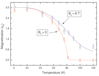
Figure 1: Theoretical results (continuous lines) and NMR implementation (open symbols) for a simple ferromagnet at $B_{0}=0$ (open squares) and $B_{0}=6$ T (open circles).

IV.2 First order phase transition

Interesting additional features appear in mean field approximation if we add an extra $M^{3}$ term in the effective magnetic field, $B=B_{0}+\lambda M+\lambda^{\prime}M^{3}$. This mean-field model presents a first order phase transition together with a thermal hysteresis, as observed in some magnetic systems livro_yeomans ; livro_lubensky . This hysteresis appears due to a difference on the behavior of the Gibbs free energy between heating up (superheating) and cooling down (supercooling) the system livro_lubensky . It is known from Landau theory that both $\lambda$ and $\lambda^{\prime}$ parameters rule the first order transition; especially the critical temperature $T_{c}$ and the superheating and supercooling temperatures (those that limit the thermal hysteresis). In other words, the occurence of the phase transition and the degree of the hysteresis depend on $\lambda$ and $\lambda^{\prime}$. Thus, being $\lambda=2(g-1)^{2}zJ_{ex}/g^{2}\mu_{B}^{2}$ with $g=2$, $z=6$, and $J_{ex}=0.5\times 10^{-19}k_{B}$, we choose $\lambda^{\prime}\ll\lambda$ (typically $\lambda^{\prime}/\lambda\sim 10^{-2}$) to obtain $T_{c}=83$ K when cooling down and $T_{c}=60$ K when heating up, which optimize the view of the phase transition and the thermal hysteresis.

In Fig.2 we show the NMR implementation of such system. The continuous lines represent the Brillouin functions and the open circles the NMR implementation. For $B_{0}=0$, the first order phase transition appears. Also in Fig.2, it can be seen the heating up of the system and the cooling down. Our NMR implementation described quite well the thermal hysteresis expected theoretically. For $B_{0}>B_{c}$, it is theoretically expected that the jump on the magnetization disappears, and our NMR implementation also described it quite well.

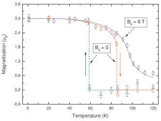
Figure 2: Theoretical results (continuous lines) and NMR implementation (open symbols). For $B_{0}=0$, the thermal hysteresis appears and is well described in the NMR system. For $B_{0}>B_{c}$ (open circles), the jump on the magnetization disappears and it is also well written on the NMR system. The open triangles are for temperature sweeping up and open squares are for temperature sweeping down.

V Conclusions

In this work we successfully described the temperature and magnetic field effects over two distinct ferromagnetic systems through NMR quantum information processing techniques: the ferromagnetic ordering described by two mean-field models. Differently from the NMR works found in literature, we directly emulated the density matrix of the ferromagnetic system by establishing a relationship between NMR spin rotations and temperature. This was done by minimizing the trace distance between the NMR and the target system density matrices. The NMR experiments correctly exhibit first and second order phase transitions, as well as thermal hysteresis. As a proof of principle, the model systems used here have analytical solution, so the main point of this article is to show that high temperature nuclear spin systems can be manipulated to behave as ordered electronic spin systems. Given that, we believe that this technique can be extended to simulate other interesting magnetic phenomena, for instance magneto-caloric effect, study of critical exponents, quantum phase transitions, etc. Particularly interesting would be the study of the environment effects over the magnetization, by looking at the magnetization phenomena.

References

- (1) A. P. Guimarães, Magnetism and Magnetic Resonance in Solids (Wiley-Interscience, New York, 1998).
- (2) J.-S. Lee and A. K. Khitrin, J. Chem. Phys. 122 (2005) 041101.
- (3) C. Negrevergne, T. S. Mahesh, C. A. Ryan, M. Ditty, F. Cyr-Racine, W. Power, N. Boulant, T. Havel, D. G. Cory, and R. Laflamme, Phys. Rev. Lett. 96 (2006) 170501.
- (4) D. G. Cory, R. Laflamme, E. Knill, L. Viola, T. F. Havel, N. Boulant, G. Boutis, E. Fortunato, S. Lloyd, R. Martinez, C. Negrevergne, M. Pravia, Y. Sharf, G. Teklemariam, Y. S. Weinstein, and W. H. Zurek, Fortschr. Phys. 48 (2000) 875.
- (5) I. S. Oliveira, T. J. Bonagamba, R. S. Sarthour, J. C. C. Freitas, and E. R. de Azevedo, NMR Quantum Information Processing (Elsevier, Amsterdam, 2007).
- (6) M. A. Nielsen, E. Knill, and R. Laflamme, Nature, 396 (1998) 52.
- (7) B. M. Fung, and V. L. Ermakov, J. Mag. Res., 166 (2004) 147.
- (8) X. Peng, J. Du, and D. Suter, Phys. Rev. A, 71 (2005) 012307.
- (9) A. M. Souza, A. Magalhães, J. Teles, E. R. deAzevedo, T. J. Bonagamba, I. S. Oliveira, and R. S. Sarthour, New J. Phys., 10 (2008) 033020.
- (10) G. A. Álvarez, E. P. Danieli, P. R. Levstein, and H. M. Pastawski, Phys. Rev. Lett., 101 (2008) 120503.
- (11) R. Auccaise, J. Teles, T. J. Bonagamba, I. S. Oliveira, E. R. deAzevedo, and R. S. Sarthour, J. Chem. Phys., 130 (2009) 144501.
- (12) S. Somaroo, C. H. Tseng, T. F. Havel, R. Laflamme, and D. G. Cory, Phys. Rev. Lett., 82 (1999) 5381.
- (13) A. K. Khitrin and B. M. Fung, Phys. Rev. A, 64 (2001) 032306.
- (14) C. Negrevergne, R. Somma, G. Ortiz, E. Knill, and R. Laflamme, Phys. Rev. A, 71 (2005) 032344.
- (15) X. Yang, A. Wang, F. Xu, and J. Du, Chem. Phys. Lett., 422 (2006) 20.
- (16) R. Das and A. Kumar, Phys. Rev. A, 68 (2003) 032304.
- (17) J. A. Jones, Prog. Nucl. Mag. Res. Sp., 38 (2001) 325.
- (18) L. M. K. Vandersypen and I. L. Chuang, Rev. Mod. Phys., 76 (2004) 1037.
- (19) J. Stolze and D. Suter, Quantum Computing: A Short Course from Theory to Experiment (Wiley-VCH, Berlin, 2008, 2nd Ed).
- (20) A. K. Khitrin and B. M. Fung, J. Chem. Phys., 112 (2000) 6963.
- (21) H. Kampermann and W. S. Veeman, Quant. Inf. Proc., 1 (2002) 327.
- (22) F. A. Bonk, E. R. deAzevedo, R. S. Sarthour, J. D. Bulnes, J. C. C. Freitas, A. P. Guimarães, I. S. Oliveira, and T. J. Bonagamba, J. Mag. Res., 175 (2005) 226.
- (23) R. Auccaise, J. Teles, R. S. Sarthour, T. J. Bonagamba, I. S. Oliveira, and E. R. deAzevedo, J. Mag. Res., 192 (2008) 17.
- (24) A. Abragam, The Principles of Nuclear Magnetism (Oxford University Press, New York, 1978).
- (25) D. Suter and T. S. Mahesh, J. Chem. Phys., 128 (2008) 052206.
- (26) R. R. Ernst, G. Bodenhausen, and A. Wokaun, Principles of Nuclear Magnetic Resonance in One and Two Dimensions (Oxford University Press, New York, 1990).
- (27) N. A. Gershenfeld, and I. L. Chuang, Science, 275 (1997) 350.
- (28) D. G. Cory, A. F. Fahmy, and T. F. Havel, Proc. Natl. Acad. Sci. USA, 94 (1997) 1634.
- (29) R. S. Sarthour, E. R. deAzevedo, F. A. Bonk, E. L. Vidoto, T. J. Bonagamba, A. P. Guimarães, J. C. Freitas, and I. S. Oliveira, Phys. Rev. A, 68 (2003) 022311.
- (30) N. Sinha, T. S Mahesh, V. K Ramanathan, and A. Kumar, J. Chem. Phys., 114 (2001) 4415.
- (31) V. L. Ermakov, and B. M. Fung. Phys. Rev. A, 66 (2002) 042310.
- (32) S. L. Braunstein, C. M. Caves, R. Jozsa, N. Linden, S. Popescu, and R. Schack. Phys. Rev. Lett., 83 (1999) 1054.
- (33) M. A. Nielsen and I. L. Chuang, Quantum Computation and Quantum Information (Cambridge University Press, Cambridge, 2000).
- (34) E. M. Fortunato, M. A. Pravia, N. Boulant, G. Teklemariam, T. F. Havel, and D. G. Cory, J. Chem. Phys., 116 (2002) 7599.
- (35) H. Kampermann and W. S. Veeman, J. Chem. Phys., 122 (2005) 214108.
- (36) T. S. Mahesh and D. Suter, Phys. Rev. A, 74 (2006) 062312.
- (37) J. Teles, E. R. deAzevedo, R. Auccaise, R. S. Sarthour, I. S. Oliveira, and T. J. Bonagamba. J. Chem. Phys., 126 (2007) 154506.
- (38) K. Radley, L. W. Reeves, and A. S. Tracey. J. Phys. Chem., 80 (1976) 174.
- (39) J. M. Yeomans, Statistical Mechanics of Phase Transitions. (Oxford University Press, New York, 1992).
- (40) P. M. Chaikin and T. C. Lubensky, Principles of Condensed Matter Physics. (Cambridge University Press, Cambridge, 1995).