MIFPA-11-11
NORDITA-2011-30
Imperial-TP-AT-2011-2
Superstrings in $AdS_{2}\times S^{2}\times T^{6}$  

We consider the type IIB Green-Schwarz superstring theory on $AdS_{2}\times S^{2}\times T^{6}$ supported by homogeneous Ramond–Ramond 5–form flux and its type IIA T–duals. One motivation is to understand the solution of this theory based on integrability. This background is a limit of a 1/4 supersymmetric supergravity solution describing four intersecting D3–branes and represents a consistent embedding of $AdS_{2}\times S^{2}$ into critical superstring theory. Its $AdS_{2}\times S^{2}$ part with corresponding fermions can be described by a classically integrable $PSU(1,1|2)/SO(1,1)\times U(1)$ supercoset sigma–model. We point out that since the RR 5–form field has non–zero components along the 6–torus directions one cannot, in general, factorize the 10d superstring theory into the supercoset part plus 6 bosons and 6 additional massless fermions. Still, we demonstrate that the full superstring model (i) is classically integrable, at least to quadratic order in fermions, and (ii) admits a consistent classical truncation to the supercoset part. Following the analogy with other integrable backgrounds and starting with the finite-gap equations of the $PSU(1,1|2)/SO(1,1)\times U(1)$ supercoset we propose a set of asymptotic Bethe ansatz equations for a subset of the quantum string states.

1 Introduction

Recent remarkable progress in exact solution of the maximally supersymmetric case of AdS/CFT duality (see, e.g., [1]) suggests applying similar integrability-based methods to other AdS/CFT systems. We are going to concentrate on the $AdS_{2}\times S^{2}$ background, whose string sigma model, we will argue, is completely integrable. The role of $AdS_{2}\times S^{2}$ as the near–horizon geometry of extremal 4d Reissner–Nordström black holes emphasizes the importance of understanding the corresponding AdS₂/CFT₁ duality [2]. There is a long and still unresolved controversy about the meaning of the corresponding “CFT₁” (a large $N$ superconformal quantum–mechanical system or a chiral “half” of a 2d CFT) [2, 3, 4, 5, 6]. One may hope to shed light on this issue by starting from the AdS₂ side, solving the corresponding string theory for any value of the radius or effective tension and re–interpreting the solution in terms of some dual CFT.

The first step is to embed the $AdS_{2}\times S^{2}$ background into critical 10d superstring theory. Requiring that the bosonic part of the string sigma model should be exactly $AdS_{2}\times S^{2}\times T^{6}$ excludes embeddings with NS–NS flux. The relevant RR–flux embedding into type IIB string theory is based on the 1/4 supersymmetric background describing four intersecting D3–branes [11]. Its “near–horizon” limit is $AdS_{2}\times S^{2}\times T^{6}$ supported, like in the $AdS_{5}\times S^{5}$ case, by a homogeneous self–dual 5–form flux. One may also consider a T–dual type IIA background, e.g., the one based on a superposition of three D4–branes and one D0–brane; in that case the $AdS_{2}\times S^{2}\times T^{6}$ space is supported by a combination of 4–form and 2–form fluxes but should lead to an equivalent string theory. The spectrum of the corresponding BPS supergravity fluctuation modes was discussed in [17, 18, 14, 19].

A natural framework for a superstring theory on a RR background such as $AdS_{2}\times S^{2}\times T^{6}$ is the Green-Schwarz (GS) formalism. The GS action is in principle defined on any supergravity background [20], although constructing it explicitly, in general, is a technically complicated problem. One needs to know the exact form of all background superfields, which can be reconstructed from the bosonic fields by solving the supergravity constraints order by order in fermions. The expressions quickly become complicated making this direct approach impractical in the absence of extra symmetries. In the $AdS_{5}\times S^{5}$ case these difficulties were effectively bypassed [21] by observing that the GS action is equivalent to a supercoset sigma model on $PSU(2,2|4)/SO(1,4)\times SO(5)$.

Following the analogy with the construction in [21] and taking into account that the superisometries of the $AdS_{2}\times S^{2}$ background form the $PSU(1,1|2)$ supergroup, ref. [22] found a formal 4d GS superstring action for the supercoset $PSU(1,1|2)/SO(1,1)\times U(1)$. A corresponding worldsheet N=2 superconformal analog based on the “standard” supercoset form of the action (with a quadratic kinetic term for the fermionic current which is absent from the GS action) was constructed in [23] where the $\mathbb{Z}_{4}$-structure of the supercoset and a local form of the Wess–Zumino term were pointed out. In addition to the supercoset part, the action of [23] included an $N=2$ superconformal theory on $CY_{3}$ (or $T^{6}$) with 6 worldsheet fermions, which is completely decoupled from the supercoset sigma–model. As we shall comment later, the relation of this “hybrid” model to the $AdS_{2}\times S^{2}\times T^{6}$ GS superstring remains an open issue.

The $PSU(1,1|2)/SO(1,1)\times U(1)$ supercoset sigma–model was interpreted in [22] as a 4d kappa–symmetry invariant GS superstring action in the $AdS_{2}\times S^{2}$ background supported by a RR 2–form flux. This supercoset action can be viewed as a direct (classical–level) truncation of the $AdS_{5}\times S^{5}$ superstring theory with only 4 bosons and 8 fermions kept non–zero and has several remarkable features. The $\mathbb{Z}_{4}$–structure [23] of the superalgebra $\mathfrak{psu}(1,1|2)$ implies [24] that this theory is also classically integrable [25] and, in addition, self–dual under the fermionic T-duality [26, 27]. In fact, its classical integrable structure is essentially equivalent to that of the $N=2$ supersymmetric sine–Gordon theory [28] as the latter is its Pohlmeyer reduction [29].

As for the quantum level, the rigid symmetry structure of this supercoset GS sigma–model implies that it should be UV finite, like its hybrid cousin in [23], and thus define a 2d conformal theory. Its one-loop beta-function was indeed shown to vanish [30] due to the vanishing Killing form of the $\mathfrak{psu}(1,1|2)$ superalgebra. There is, however, an obvious problem with interpreting the coset sigma-model as a critical string theory. The standard central charge count in a critical flat–space GS theory is (see, e.g., [31]): $c_{tot}=(n_{b}+2)-26+{\frac{1}{2}}\times 4\times n_{f}$ where $n_{b}$ and $n_{f}$ are the numbers of physical bosonic and fermionic degrees of freedom. While for the 10d superstring one has $n_{b}=n_{f}=8$ implying $c_{tot}=0$ for the 4d GS string one gets $c_{tot}=(2+2)-26+{\frac{1}{2}}\times 4\times 2=-18$. One may try to cancel the central charge deficit by adding extra decoupled bosons and fermions but while this may be straightforward in the NSR framework it is not clear a priori how this can be consistently implemented in the GS case. An alternative is to use the “hybrid” model of [23] but as mentioned its equivalence to the critical 10d superstring theory remains an open question.

In this paper we propose to start directly with a critical 10d superstring theory defined in the $AdS_{2}\times S^{2}\times T^{6}$ background supported by RR flux and explore its relation to the above supercoset theory. Since, e.g., in the type IIB embedding [11] the $F_{5}$ flux has non–zero components along the $T^{6}$ directions the toroidal string coordinates do not a priori decouple from the GS fermions. This non-decoupling of the “flat directions” sets the $AdS_{2}\times S^{2}\times T^{6}$ case apart from the previously studied coset-type critical-string backgrounds, where additional degrees of freedom could be either completely eliminated ($AdS_{4}\times CP^{3}$) or decoupled ($AdS_{3}\times S^{3}\times T^{4}$) from the coset by an appropriate choice of kappa-symmetry gauge. Contrary to what one might expect, in the present case it will not be possible to represent the world-sheet sigma-model as a direct sum of the $PSU(1,1|2)/SO(1,1)\times U(1)$ supercoset and additional free bosonic and fermionic modes. However, as we will show later, the GS action admits a reduction to the supercoset theory in a weaker sense as a classically consistent truncation.

The mixing between the coset and flat directions of $T^{6}$ may cast doubts on the potential integrability of the model, beyond the coset truncation. We shall find that quite remarkably the full superstring theory in the supersymmetric $AdS_{2}\times S^{2}\times T^{6}$ backgrounds is also classically integrable. Following [32] we shall construct the Lax connection (to quadratic order in fermions) from the components of the conserved currents of the full GS action. We will show that the flatness condition for this Lax connection is equivalent to the full set of equations of motion of the GS superstring, thus proving classical integrability of the string sigma-model. If integrability is not spoiled at the quantum level, the theory may eventually be solvable by Bethe ansatz techniques.

As a first step towards the exact solution, we derive the classical counterpart of the Bethe equations that describe finite–gap classical solutions of the supercoset sigma–model. Under the assumption that the supercoset truncation goes through also at the level of massive quantum states with large quantum numbers we propose a set of asymptotic Bethe equations for part of the quantum spectrum of the theory. We shall also discuss some preliminary consistency checks of integrability based on a 1-loop semiclassical expansion.

This paper is organized as follows. In Section 2 we shall start with the action of a $D=10$ GS superstring in a general symmetric–space background supported by RR fluxes written to quadratic order in fermions and find the conditions for its classical integrability to this order by constructing a candidate Lax connection in terms of the Noether isometry currents.

In Section 3 we shall consider explicit examples of type IIA and type IIB backgrounds with $AdS_{2}\times S^{2}\times T^{6}$ supported by RR fluxes and verify that the conditions for classical integrability of the corresponding GS superstring action are satisfied, at least to quadratic order in fermions.

In Section 4 we show that the type II GS string action for the $AdS_{2}\times S^{2}\times T^{6}$ backgrounds preserving eight supersymmetries can be consistently truncated, at the classical level, to the $PSU(1,1|2)/SO(1,1)\times U(1)$ supercoset GS sigma–model with $AdS_{2}\times S^{2}$ as bosonic part and eight fermionic modes. We shall first show this to quadratic order in fermions and then extend the argument to all orders.

In Section 5 we shall consider two inequivalent BMN limits of the superstring action: When the center of mass (c.o.m.) of the string is moving along a big circle of $S^{2}$ or when it moves both in $S^{2}$ and in $S^{1}\subset T^{6}$. The first case corresponds to the BPS vacuum state of the theory and preserves 1/2 of the original supersymmetry. The unbroken supersymmetry can be recast in the 2d form, and leads to the Bose-Fermi degeneracy of the BMN modes. The non-coset degrees of freedom remain massless in this limit. In the second case the gauge–fixed sigma–model does not have effective 2d supersymmetry, and the degeneracy is lifted. Moreover, some of the ‘non–supercoset’ fermions acquire mass in this case.

In Section 6 we shall first review the classical Bethe equations describing finite gap solutions of the $PSU(1,1|2)/SO(1,1)\times U(1)$ supercoset model [33] and then propose a set of quantum asymptotic Bethe equations that potentially describe the spectrum of the string in the light-cone gauge associated with the supersymmetric BMN geodesic. These equations, however, only describe a subset of the massive states and do not capture the massless, non-coset degrees of freedom.

In Section 7 we discuss various semiclassical string solutions in $AdS_{2}\times S^{2}\times T^{6}$ and clarify the validity of the assumption of decoupling of the $AdS_{2}\times S^{2}$ sector.

There are several Appendices describing our notation, the structure of the (enlarged) $\mathfrak{psu}(1,1|2)$ superalgebra and properties of Killing vectors on symmetric spaces. In Appendix D we also provide details of the derivation of the classical string equations of motion from the flatness of the Lax connection constructed in Section 2.

2 GS superstrings in RR backgrounds and their
classical integrability

A particular feature of GS superstrings propagating in supersymmetric backgrounds whose geometry is a direct product of an AdS space with compact manifolds is that (at least part of) their dynamics can often be described by certain supercoset sigma–models whose isometry superalgebras have a $\mathbb{Z}_{4}$–grading. For example, the $PSU(2,2|4)/SO(1,4)\times SO(5)$ sigma–model defines the maximally supersymmetric type IIB $AdS_{5}\times S^{5}$ superstring theory [21]. Also, an $OSp(6|4)/SO(1,3)\times U(3)$ sigma–model with 24 supersymmetries [34, 35] represents the type IIA $AdS_{4}\times CP^{3}$ superstring in those sectors where a partial kappa–symmetry gauge fixing is allowed to reduce the complete GS action to the $OSp(6|4)/SO(1,3)\times U(3)$ sigma–model one containing 24 worldsheet fermions [34, 36, 37, 38].

In the case of an $AdS_{3}\times S^{3}\times T^{4}$ background supported by RR 3-form flux which preserves 16 out of the 32 possible supersymmetries, one can reduce the GS action to a sigma–model on the supercoset $PSU(1,1|2)\times PSU(1,1|2)/SU(1,1)\times SU(2)$ (which has $AdS_{3}\times S^{3}$ as its bosonic subspace) plus the decoupled free bosonic sector on $T^{4}$ [39]. To this end one should completely gauge fix the kappa–symmetry by eliminating 16 of the 32 fermionic modes of the 10d GS superstring in an appropriate way. For some “singular” classical string configurations (e.g., when the string does not wind or move in $T^{4}$) such kappa–symmetry gauge fixing is inadmissible. In such special cases there are physical fermionic degrees of freedom which are not part of the supercoset sigma–model and to take them into account one should start with the complete 10d GS superstring action.

The situation turns out to be more complicated in the case of $AdS_{2}\times S^{2}\times T^{6}$ backgrounds. The GS sigma–model on $PSU(1,1|2)/SO(1,1)\times U(1)={\rm Super}(AdS_{2}\times S^{2})$ [22] indeed possesses a $\mathbb{Z}_{4}$–grading [23] and is thus classically integrable [24], much like the GS sigma-models on $AdS_{5}\times S^{5}$, $AdS_{4}\times CP^{3}$ and $AdS_{3}\times S^{3}\times T^{4}$. The crucial difference is in the number of preserved supersymmetries. The $\mathfrak{psu}(1,1|2)$ superalgebra has only 8 supercharges, compared to 32 for $AdS_{5}\times S^{5}$, 24 for $AdS_{4}\times CP^{3}$ and 16 for $AdS_{3}\times S^{3}\times T^{4}$. As a result, the 16-parametric kappa–symmetry of the GS action is not sufficient to gauge away the additional $32-8=24$ worldsheet fermions associated with broken 10d supersymmetries. At least 8 of the broken-symmetry fermions will remain in the physical spectrum of the string, and will link the decoupled, at first sight, $T^{6}$ sector to the coset.

Since extra, non-coset degrees of freedom cannot be gauged away and do not decouple, the integrability of the supercoset is not sufficient to prove the integrability of the full theory which includes the fermions associated with broken supersymmetries. To analyze integrability, we will follow an alternative approach, proposed for the type IIA superstring action on $AdS_{4}\times CP^{3}$ [32]. In this approach, the Lax connection is constructed directly from the Noether currents of the full superstring action without requiring that the string sigma–model has a coset structure. We will demonstrate that (at least up to the second order in all the 32 fermions) the type II $D=10$ GS superstring propagating in $AdS_{2}\times S^{2}\times T^{6}$ background (supported by type IIA or type IIB RR fluxes) is classically integrable. Thus the integrability still applies despite the fact that the integrable $PSU(1,1|2)/SO(1,1)\times U(1)$ sigma–model cannot give a complete description of the GS superstring in the $AdS_{2}\times S^{2}\times T^{6}$ case.

We shall also show that in the non–supersymmetric $AdS_{2}\times S^{2}\times T^{6}$ backgrounds which are obtained from the supersymmetric ones by changing signs of some components of the RR fluxes, the same prescription for the construction of the Lax connection fails already at the quadratic order in fermions.

In this section we will consider a $D=10$ GS superstring in a generic superbackground with non–zero RR fluxes whose bosonic subspace is a symmetric space. We will derive relations that should be satisfied by components of the Noether currents of the background superisometries in order to be able to construct from them a zero–curvature Lax connection, up to the second order in fermions. We then show that the type II superstrings in the $AdS_{2}\times S^{2}\times T^{6}$ backgrounds satisfy these requirements and hence are classically integrable, at least to quadratic order in fermions.

To construct a complete Lax connection to all orders in fermions one should know the explicit form of the full GS superstring action. A derivation of such an explicit form of the GS action in a $D=10$ superbackground which is not maximally supersymmetric turns out to be a technically complicated problem. So far it has been solved only for two cases which can be obtained by double dimensional reduction of the supermembrane action in corresponding $D=11$ maximally supersymmetric backgrounds: a locally flat one and $AdS_{4}\times S^{7}$. They correspond to, respectively, the type IIA superstring in a 7–brane background with a magnetic RR flux [40] and to the type IIA superstring in the $AdS_{4}\times CP^{3}$ superbackground [36] (the latter is the extension to superspace of the Hopf fibration realization of the $D=11$ supergravity solution [41, 42, 43]).

2.1 GS superstrings in RR backgrounds, equations of motion and conserved currents

The action for the GS superstring in a bosonic supergravity background (with zero NS–NS flux and constant dilaton $\phi$) has the following form up to quadratic order in fermions [44, 45]

$$S=-T\int\left(\frac{1}{2}\ast e^{A}e_{A}+i\ast e^{A}\,\Theta\Gamma_{A}{\mathcal{D}}\Theta-ie^{A}\,\Theta\Gamma_{A}\hat{\Gamma}\,{\mathcal{D}}\Theta\right)\,,$$ (2.1)

where $e^{A}(X)$ $(A=0,1,\cdots,9)$ are worldsheet pull–backs of the background vielbein one–forms and

$${\mathcal{D}}\Theta=(\nabla-\frac{1}{8}e^{A}\,\not{F}\Gamma_{A})\Theta\,,$$ (2.2)

is the fermionic vielbein to the lowest order in fermions $\Theta$. Here $\nabla=d+\omega$ is the covariant derivative containing the spin connection of the background space–time,

$$\hat{\Gamma}=\left\{\begin{array}[]{c}\Gamma_{11}\\ \sigma^{3}\end{array}\right.\begin{array}[]{c}(\mathrm{IIA})\\ (\mathrm{IIB})\end{array}$$ (2.3)

and the coupling to the RR fields is given in terms of the matrix

$$\not{F}=e^{\phi}\left\{\begin{array}[]{c}-\frac{1}{2}\Gamma^{AB}\Gamma_{11}F_{AB}+\frac{1}{4!}\Gamma^{ABCD}F_{ABCD}\\ {}\hfil\\ i\sigma^{2}\Gamma^{A}F_{A}-\frac{1}{3!}\sigma^{1}\Gamma^{ABC}F_{ABC}+\frac{i}{2\cdot 5!}\sigma^{2}\Gamma^{ABCDE}F_{ABCDE}\end{array}\right.\begin{array}[]{c}(\mathrm{IIA})\\ {}\hfil\\ (\mathrm{IIB})\end{array}$$ (2.4)

in the type IIA and type IIB case, respectively. We describe the two Majorana–Weyl spinors in the IIA case as one 32-component Majorana spinor $\Theta$ and in the IIB case as two 32-component Majorana spinors projected onto one chirality $\Theta^{i}$ ($i=1,2$) by $\frac{1}{2}(1+\Gamma_{11})$. The Pauli matrices $\sigma^{1},\sigma^{2}$ and $\sigma^{3}$ act on the IIB SO(2)–indices $i,j=1,2$ which will be suppressed.

The bosonic equations of motion to the second order in $\Theta$ are then

$$\nabla\left(*(e^{A}+i\Theta\Gamma^{A}{\mathcal{D}}\Theta)+i\Theta\Gamma^{A}\hat{\Gamma}\,{\mathcal{D}}\Theta-\frac{i}{8}*e^{B}\,\Theta\Gamma^{A}\not{F}\Gamma_{B}\Theta-\frac{i}{8}e^{B}\,\Theta\Gamma^{A}\hat{\Gamma}\not{F}\Gamma_{B}\Theta\right)$$ (2.5)

$$-\frac{i}{4}*e^{B}e^{E}\,\Theta\Gamma_{B}{}^{CD}\Theta\,R_{CDE}{}^{A}+\frac{i}{4}e^{B}e^{E}\,\Theta\Gamma_{B}{}^{CD}\hat{\Gamma}\Theta\,R_{CDE}{}^{A}=0\,,$$

where $R_{CDE}{}^{A}(X)$ is the curvature of the $D=10$ space, and the fermionic equations (linear in $\Theta$) are

$$(\ast e^{A}\,\Gamma_{A}-e^{A}\,\Gamma_{A}\hat{\Gamma})\,{\mathcal{D}}\Theta=0\,.$$ (2.6)

If the background has bosonic isometries, generated by Killing vectors $K_{A}(X)$, the worldsheet model has the corresponding conserved Noether current one–form of the following generic form (see [32] for more details)

$$J_{\mathcal{B}}=J^{A}K_{A}+J^{AB}\nabla_{A}K_{B}=e^{A}K_{A}+\mbox{fermions}\,,$$ (2.7)

where the second term comes from compensating Lorentz transformations of the fermionic fields $\Theta$. The $J^{A}$ and $J^{AB}$ terms in the current have the following form

$$J^{A}=e^{A}+i\Theta\Gamma^{A}{\mathcal{D}}\Theta-\frac{i}{8}e^{B}\,\Theta\Gamma^{A}\not{F}\Gamma_{B}\Theta+i\Theta\Gamma^{A}\hat{\Gamma}\ast\mathcal{D}\Theta-\frac{i}{8}*e^{B}\,\Theta\Gamma^{A}\hat{\Gamma}\not{F}\Gamma_{B}\Theta\,,$$ (2.8)

$$J^{AB}=\frac{1}{4}(\Gamma^{AB}\Theta)^{\alpha}\ast i_{\alpha}\mathcal{L}=-\frac{i}{4}e^{C}\,\Theta\Gamma^{AB}{}_{C}\Theta+\frac{i}{4}\ast e^{C}\,\Theta\Gamma^{AB}{}_{C}\hat{\Gamma}\Theta\,,$$ (2.9)

where $\mathcal{L}$ is the superstring Lagrangian in (2.1).

If the background preserves some supersymmetries generated by Killing spinors $\Xi(X)$, there is also a conserved supersymmetry current on the worldsheet which to linear order in $\Theta$ has the following form

$$J_{susy}=\frac{i}{2R}(e^{A}\,\Theta\Gamma_{A}\Xi-\ast e^{A}\,\Theta\Gamma_{A}\hat{\Gamma}\Xi)\,,$$ (2.10)

where the dimension–of–length constant $R$ (which in our case will be the AdS radius) has been introduced to make the current dimensionless, and $\Xi$ satisfies the Killing spinor equation

$$\nabla\Xi-\frac{1}{8}e^{A}\,\not{F}\Gamma_{A}\Xi=0\,.$$ (2.11)

As usual, the currents (2.7) and (2.10) are conserved

$$d*J_{\mathcal{B}}=0,\qquad d*J_{susy}=0,$$ (2.12)

provided that the equations of motion (2.5) and (2.6) are satisfied (and vice versa). The conservation of (2.7) and orthogonality of $K_{A}$ and $\nabla_{A}K_{B}=[K_{A},K_{B}]$ imply that the following relations must hold separately (see Appendix C for basic relations satisfied by the Killing vectors of a symmetric space)

$$(\nabla\ast J^{AB}-\ast J^{[A}e^{B]})K_{A}\,K_{B}=0\,,$$ (2.13)

$$\nabla\ast J^{A}-2R_{BCD}{}^{A}\ast J^{CD}e^{B}=0\,.$$ (2.14)

2.2 Lax connection built from conserved currents

In many examples of interest, such as $AdS_{4}\times CP^{3}$, $AdS_{2}\times S^{2}\times T^{6}$ or $AdS_{3}\times S^{3}\times T^{4}$, the complete target superspace describing the superstring background is not a supercoset manifold, so the $\mathbb{Z}_{4}$–graded supercoset prescription of ref. [24] for the construction of the Lax connection does not directly apply. In [32] an alternative prescription was proposed for these cases and applied to $AdS_{4}\times CP^{3}$. It uses the conserved currents as building blocks. The Lax connection has two parts

$$L=L_{\mathcal{B}}+L_{\mathcal{F}}\,.$$ (2.15)

The part $L_{\mathcal{B}}$ of the Lax connection that corresponds to the bosonic isometries has the following form (similar to (2.7))

$$L_{\mathcal{B}}=L^{A}K_{A}+L^{AB}\nabla_{A}K_{B}\,,$$ (2.16)

where

$$L^{A} = \alpha_{1}\,e^{A}+\alpha_{2}\ast J^{A},$$ (2.17)

$$L^{AB} = \alpha_{2}^{2}\,J^{AB}+\alpha_{2}(1+\alpha_{1})\ast J^{AB}\,.$$ (2.18)

The part corresponding to the fermionic isometries is

$$L_{\mathcal{F}}=-\alpha_{2}\beta_{1}J_{susy}+\alpha_{2}\beta_{2}\ast J_{susy}\,.$$ (2.19)

The numerical parameters $\alpha_{1}$, $\alpha_{2}$, $\beta_{1}$ and $\beta_{2}$ are expressed in terms of a single spectral parameter by requiring that the Lax connection (2.15) has zero curvature

$$dL-LL=0\,.$$ (2.20)

In fact, the values of $\alpha_{1}$ and $\alpha_{2}$ are determined in terms of the spectral parameter already by the requirement of integrability of the purely bosonic part of the superstring sigma–model. One can check that if in (2.16) we put $\Theta$ to zero, the Lax connection reduces to its conventional form for an integrable sigma–model on a symmetric space [46]:

$$L_{\mathcal{B}}|_{\Theta=0}=(\alpha_{1}e^{A}+\alpha_{2}\ast e^{A})K_{A}\,.$$

The curvature of this connection vanishes if

$$\alpha_{2}^{2}=2\alpha_{1}+\alpha_{1}^{2}\,\qquad\Rightarrow\qquad\alpha_{1}=\frac{2{\tt x}^{2}}{1-{\tt x}^{2}},\qquad\alpha_{2}=\pm\frac{2{\tt x}}{1-{\tt x}^{2}},$$ (2.21)

where ${\tt x}$ is the spectral parameter. When the fermionic fields are non–zero, using the equations of motion we find that up to the quadratic order in fermions the $L_{\mathcal{B}}$–terms in the curvature (2.20) proportional to the Killing vectors $K_{A}$ are

$$(dL_{\mathcal{B}}-L_{\mathcal{B}}L_{\mathcal{B}})^{A} = 2\alpha_{2}(\alpha_{2}^{2}-2\alpha_{1}-\alpha_{1}^{2})\,R_{BCD}{}^{A}\ast J^{CD}e^{B}\,.$$ (2.22)

We observe that the right-hand-side of (2.22) vanishes when the parameters satisfy eq. (2.21). The $L_{\mathcal{B}}$–terms of the Lax curvature proportional to the derivative of the Killing vectors $\nabla_{A}K_{B}$ are

$$(dL_{\mathcal{B}}-L_{\mathcal{B}}L_{\mathcal{B}})^{AB}=\alpha_{2}^{2}\Big{[}\nabla J^{AB}+(J-e)^{[A}e^{B]}\Big{]}\,.$$ (2.23)

If the right-hand-side of (2.23) vanishes then $L_{\mathcal{B}}$ has zero curvature and may itself play the role of the Lax connection (i.e. in (2.15) the term $L_{\mathcal{F}}$ can be set to zero). An example, when this happens is an integrable non–supersymmetric GS superstring on $AdS_{4}$ considered in [32]. In this case there is no supersymmetry Noether current (2.10).

However, in general, the right-hand-side of (2.23) is non–zero. Then we need to show that these terms in the curvature can be cancelled by adding other terms to the Lax connection. When the background possesses some supersymmetry these additional terms are built from the supersymmetry current (2.10) and have the form given in (2.19). This is what happened in $AdS_{4}\times CP^{3}$ [32]. It will be possible to cancel the curvature of the Lax connection by this mechanism for the $AdS_{2}\times S^{2}\times T^{6}$ backgrounds as well.

To see if the curvature term (2.23) can be canceled by contributions from (2.19), let us compute the curvature of the total Lax connection (2.15) for the parameters $\alpha_{1}$ and $\alpha_{2}$ related by (2.21)

$$dL-LL = \alpha_{2}^{2}(\nabla J^{AB}+(J^{A}-e^{A})e^{B})\nabla_{A}K_{B}+\alpha_{2}^{2}(\beta_{2}^{2}-\beta_{1}^{2})J_{susy}^{2}-\alpha_{2}\beta_{1}dJ_{susy}$$ (2.24)

$${}+\alpha_{2}(\alpha_{1}\beta_{1}+\alpha_{2}\beta_{2})(J_{\mathcal{B}}J_{susy}+J_{susy}J_{\mathcal{B}})$$

$${}-\alpha_{2}(\alpha_{1}\beta_{2}+\alpha_{2}\beta_{1})(J_{\mathcal{B}}\ast J_{susy}+\ast J_{susy}J_{\mathcal{B}})\,.$$

Now, if

$$\beta_{1}=\mp\sqrt{\frac{\alpha_{1}}{2}}=\pm\frac{i{\tt x}}{\sqrt{{\tt x}^{2}-1}}\,,\qquad\beta_{2}=\pm\frac{\alpha_{2}}{\sqrt{2\alpha_{1}}}=\mp\frac{i}{\sqrt{{\tt x}^{2}-1}}\,$$ (2.25)

the last term in eq. (2.24) vanishes and the other terms cancel each other provided that

$$dJ_{susy}=-2(J_{\mathcal{B}}J_{susy}+J_{susy}J_{\mathcal{B}}),$$ (2.26)

and

$$\left[\nabla J^{AB}+(J^{A}-e^{A})e^{B}\right]\nabla_{A}K_{B}=-J_{susy}^{2}\,.$$ (2.27)

These equations can be viewed as a modified version of the familiar Maurer-Cartan equation $dJ=-2J^{2}$, with $J=J_{\mathcal{B}}+\frac{1}{\sqrt{2}}J_{susy}$ and with some terms proportional to $K_{A}$ removed.

Verifying that eqs. (2.26) and (2.27) hold is therefore enough to demonstrate the integrability at this order. We will see below that just as in the $AdS_{4}\times CP^{3}$ case these equations hold for strings in $AdS_{2}\times S^{2}\times T^{6}$. Let us first compute the left-hand-sides of these equations in a general RR background. Using the form of the supersymmetry current (2.10) and the equations of motion we get

$$dJ_{susy}=\frac{i}{8R}(e^{A}e^{B}\,\Theta\Gamma_{A}\not{F}\Gamma_{B}\Xi-\ast e^{A}e^{B}\,\Theta\Gamma_{A}\hat{\Gamma}\not{F}\Gamma_{B}\Xi)\,.$$ (2.28)

Using the form (2.9) of $J^{AB}$ we find that

$$\nabla J^{AB} = -\frac{i}{2}e^{C}\,\Theta\Gamma^{AB}{}_{C}\nabla\Theta+\frac{i}{2}\ast e^{C}\,\Theta\Gamma^{AB}{}_{C}\hat{\Gamma}\nabla\Theta$$ (2.29)

$$= ie^{[B}\,\Theta\Gamma^{A]}\nabla\Theta-i\ast e^{[B}\,\Theta\Gamma^{A]}\hat{\Gamma}\nabla\Theta-\frac{i}{16}e^{C}e^{D}\,\Theta\Gamma^{AB}\Gamma_{C}\not{F}\Gamma_{D}\Theta$$

$${}+\frac{i}{16}\ast e^{C}e^{D}\,\Theta\Gamma^{AB}\Gamma_{C}\hat{\Gamma}\not{F}\Gamma_{D}\Theta\,,$$

where we have made use of the equations of motion. We can further rewrite this as

$$\nabla J^{AB}+e^{[A}(J^{B]}-e^{B]})=-\frac{i}{16}e^{C}e^{D}\,\Theta\Gamma_{C}\Gamma^{AB}\not{F}\Gamma_{D}\Theta+\frac{i}{16}\ast e^{C}e^{D}\,\Theta\Gamma_{C}\Gamma^{AB}\hat{\Gamma}\not{F}\Gamma_{D}\Theta\,.$$ (2.30)

As we have seen, for the Lax–connection curvature (2.24) to vanish the right-hand-side of (2.30) should be the square of $J_{susy}$ and the right-hand-side of (2.28) should be the commutator of $J_{\mathcal{B}}$ with $J_{susy}$. In the next section we will show that this holds for various $AdS_{2}\times S^{2}\times T^{6}$ solutions with RR fluxes which preserve eight supersymmetries.

3 Superstrings in $AdS_{2}\times S^{2}\times T^{6}$ backgrounds

As we have discussed in the Introduction, there are several solutions of type IIA and type IIB supergravity with the geometry of $AdS_{2}\times S^{2}\times T^{6}$ supported by RR fluxes which are related by $T$-duality. Type IIA solutions are also related by dimensional reduction to certain $AdS_{n}\times S^{k}\times T^{m}$ solutions of $D=11$ supergravity which correspond to limits of configurations of intersecting M2– and M5–branes (that upon compactification describe $D=4$ black holes) [11].

We start from the most symmetric configuration which consists of four intersecting $D3$-branes in type IIB string theory. The setup is as follows (with $\times$ indicating the directions along the branes)

$$\begin{array}[]{ll|c|cccccc}&AdS_{2}&S^{2}&&&T^{6}&&&\\ \hline\cr&0\quad 1&2\quad 3&4&5&6&7&8&9\\ \hline\cr D3&\times&&\times&\times&\times&&&\\ D3&\times&&\times&&&\times&\times&\\ D3&\times&&&\times&&&\times&\times\\ D3&\times&&&&\times&\times&&\times\\ \hline\cr\end{array}$$ (3.1)

and the $F_{5}$–flux is given in (3.18). By performing T-dualities on some of the $T^{6}$-directions we can obtain different solutions. In particular, T–dualizing along one of the $T^{6}$ directions, say $y^{4}$, gives a configuration with two $D2$ and two $D4$-branes and electric and magnetic $F_{4}$-flux given in (3.15) in type IIA. Similarly T-dualizing the (456)-directions gives one $D0$ and three $D4$-branes with electric $F_{2}$-flux and magnetic $F_{4}$-flux given in (3.2), while T-dualizing the (789)-directions instead gives one $D6$ and three $D2$-branes with magnetic $F_{2}$-flux and electric $F_{4}$-flux given in (3.1).

We will consider these solutions in more detail below and verify explicitly the integrability of the GS superstring in the IIA background with electric $F_{2}$ and magnetic $F_{4}$–flux as well as in the IIB background with $F_{5}$–flux to quadratic order in fermions. Since the two backgrounds are related by T–duality it should of course not be necessary to perform this analysis in both cases, however we find this worth doing since there are interesting differences between the two cases in how, for example, the $\mathfrak{psu}(1,1|2)$-algebra is realized. This also gives a useful consistency check of our results.

3.1 Type IIA $AdS_{2}\times S^{2}\times T^{6}$ with $F_{2}$ and $F_{4}$ flux

This 1/4 supersymmetric $AdS_{2}\times S^{2}\times T^{6}$ solution of type IIA supergravity is supported by the following combination of the RR 2-form and 4-form fluxes

$$F_{2} = -\frac{e^{-\phi}}{2R}e^{b}e^{a}\varepsilon_{ab}\,,$$

$$F_{4} = -\frac{e^{-\phi}}{2R}e^{\hat{b}}e^{\hat{a}}\varepsilon_{\hat{a}\hat{b}}J_{2}\,,$$ (3.2)

where $\phi$ is the (constant) dilaton, $J_{2}=\frac{1}{2}dy^{b^{\prime}}dy^{a^{\prime}}J_{a^{\prime}b^{\prime}}$ is the Kähler form on $T^{6}$, $\varepsilon^{01}=1$, $R$ is the radius of $AdS_{2}$ and $S^{2}$, and $a,b=0,1$, $\hat{a},\hat{b}=2,3$ and $a^{\prime},b^{\prime}=4,\ldots,9$ are the $AdS_{2}$, $S^{2}$ and $T^{6}$ indices, respectively.

There is also a solution with the roles of the two fluxes interchanged, i.e.

$$F_{2} = \frac{e^{-\phi}}{2R}e^{\hat{b}}e^{\hat{a}}\varepsilon_{\hat{a}\hat{b}}\,,$$

$$F_{4} = -\frac{e^{-\phi}}{2R}e^{b}e^{a}\varepsilon_{ab}J_{2}\,.$$ (3.3)

This solution can be obtained by reduction from the 1/4 supersymmetric $D=11$ supergravity solution $AdS_{2}\times S^{3}\times T^{6}$ with the same $F_{4}$–flux. This is done by realizing $S^{3}$ as an $S^{1}$ Hopf fibration over $S^{2}$. Dimensionally reducing on this $S^{1}$ creates an $F_{2}$–flux proportional to the Kähler form on $S^{2}\sim CP^{1}$ similar to what happens in the $AdS_{4}\times CP^{3}$ case. In a similar way, the type IIA solution (3.2) is the dimensional reduction of the 1/4 supersymmetric $D=11$ supergravity solution $AdS_{3}\times S^{2}\times T^{6}$ with $F_{4}=-\frac{1}{2R}e^{\hat{b}}e^{\hat{a}}\varepsilon_{\hat{a}\hat{b}}J_{2}$.

Note that if we change the sign of one of the fluxes in (3.2) or (3.1), the $AdS_{2}\times S^{2}\times T^{6}$ space will still be a solution of the supergravity equations of motion, but the supersymmetry will be completely broken. This supersymmetry breaking is reflected in the form of $\not{F}$ in (2.4) which will no longer be proportional to a projector. This will also spoil the structure of the Lax connection discussed in the previous section; in the non–supersymmetric cases we have not been able to make it have zero curvature since it does not appear to be possible to cancel the terms on the right–hand–side of eq. (2.23) without a supersymmetry current. This may indicate that, though the purely bosonic sector of these non–supersymmetric models is classically integrable, the integrability is spoiled by the fermionic sector.

Let us now consider the structure of the superisometry algebra $\mathfrak{psu}(1,1|2)$ of the background (3.2) and demonstrate that it ensures the vanishing of the curvature of the Lax connection (2.15) (the analysis of the background (3.1) can be carried out in exactly the same fashion). For the supersymmetric solution (3.2) the definition of $\not{F}$ in eq. (2.4) gives

$$\not{F}=-\frac{1}{R}\gamma\Gamma_{11}+\frac{i}{2R}\gamma\gamma^{5}\Gamma^{a^{\prime}b^{\prime}}J_{a^{\prime}b^{\prime}}=-\frac{4}{R}\mathcal{P}_{8}\gamma\Gamma_{11}\,,$$ (3.4)

$$\mathcal{P}_{8}=\frac{1}{8}(2-iJ_{a^{\prime}b^{\prime}}\Gamma^{a^{\prime}b^{\prime}}\gamma^{7})\,,$$ (3.5)

where $\gamma=\Gamma^{0}\Gamma^{1}$ is the product of $AdS_{2}$ gamma matrices (so that $\gamma^{2}=1$) and $\gamma^{5}=i\Gamma^{0}\Gamma^{1}\Gamma^{2}\Gamma^{3}$. Here $\mathcal{P}_{8}$ is a projector which for all the $AdS_{2}\times S^{2}\times T^{6}$ solutions has the following properties: it commutes with the $D=10$ matrices $\Gamma^{a}$ $(a=0,1)$ and $\Gamma^{\hat{a}}$ $(\hat{a}=2,3)$ along the $AdS_{2}\times S^{2}$ directions, as well as with $\hat{\Gamma}$ ($=\Gamma_{11}$ in the IIA case)

$$[\mathcal{P}_{8},\Gamma^{a}]=[\mathcal{P}_{8},\Gamma^{\hat{a}}]=[\mathcal{P}_{8},\hat{\Gamma}]=0\,,$$ (3.6)

while for $\Gamma^{a^{\prime}}$ with $a^{\prime}=4,\ldots,9$ along the $T^{6}$ directions we have

$$\mathcal{P}_{8}\Gamma^{a^{\prime}}\mathcal{P}_{8}=0\,.$$ (3.7)

The projector $\mathcal{P}_{8}$ singles out an eight–dimensional supersymmetric subspace of the 32 dimensional fermionic space and is defined in a similar way to the $CP^{3}$ case [41, 36] but with the Kähler form of $CP^{3}$ replaced by that of $T^{6}$.

As we shall see, the same projector appears in the $\mathfrak{psu}(1,1|2)$ superalgebra of the superisometries and so the extra terms in $\nabla J^{AB}$, eqs. (2.27) and (2.30), are of the required form to be canceled by the terms coming from $J_{susy}^{2}$. A conventional form of the $\mathfrak{psu}(1,1|2)$ algebra given in eq. (B.9) of Appendix B differs from what we would like to have in this case by factors of $\gamma^{5}$. A way to cure this is to take a slightly different realization of the gamma matrices in the algebra (B.9) which, of course, is an automorphism of the algebra. Taking

$$\Gamma^{a} \rightarrow i\Gamma^{a}\gamma^{5},$$

$$\Gamma^{\hat{a}} \rightarrow i\Gamma^{\hat{a}}\gamma^{5},$$

$$\Gamma^{a^{\prime}} \rightarrow \Gamma^{a^{\prime}}$$ (3.8)

together with the redefinition of the charge conjugation matrix $\mathcal{C}\rightarrow i\mathcal{C}\gamma^{5}$ preserves the Clifford algebra, symmetry properties of the gamma matrices and the form of the projector $\mathcal{P}_{8}$. The commutators involving $Q=\mathcal{P}_{8}Q$ in the $\mathfrak{psu}(1,1|2)$ algebra (B.9) now become

$$[P_{A},Q] = \frac{1}{2R}Q\gamma\Gamma_{11}\Gamma_{A}\mathcal{P}_{8}\ ,\qquad[M_{AB},Q]=-\frac{1}{2}Q\Gamma_{AB}\mathcal{P}_{8}$$

$$\{Q,Q\} = 2i(\mathcal{P}_{8}\Gamma^{A}\mathcal{P}_{8})P_{A}+\frac{iR}{2}(\mathcal{P}_{8}\Gamma^{AB}\gamma\Gamma_{11}\mathcal{P}_{8})R_{AB}{}^{CD}M_{CD}\,,$$ (3.9)

and have the required form since they contain $\not{F}\propto\mathcal{P}_{8}\gamma\Gamma_{11}$.

The relations between the Killing vectors $K_{A}$ and the Killing spinors $\Xi$ and the generators of the algebra are

$$K_{A}=kP_{A}k^{-1},\qquad i\mathcal{C}\gamma\Gamma_{11}\Xi=kQk^{-1}$$ (3.10)

$$\nabla_{A}K_{B}=-\frac{1}{2}R_{AB}{}^{CD}kM_{CD}k^{-1}\,,$$ (3.11)

where $k(x)$ is a coset element of $SO(1,2)\times SU(2)/SO(1,1)\times U(1)$ and the Killing vectors $K_{a^{\prime}}=P_{a^{\prime}}$ generate the translation isometries of $T^{6}$.

Using these relations we have

$$\{\Xi,\Xi\} = 2i(\gamma\mathcal{P}_{8}\Gamma^{A}\mathcal{P}_{8}\gamma\mathcal{C})K_{A}+iR(\mathcal{P}_{8}\Gamma^{AB}\gamma\Gamma_{11}\mathcal{P}_{8}\mathcal{C})\nabla_{A}K_{B}$$

$${}[K_{A},\Xi] = -\frac{1}{2R}\Xi\Gamma_{A}\mathcal{P}_{8}\gamma\Gamma_{11}\mathcal{C}\,.$$ (3.12)

Note that along the $T^{6}$ directions $\nabla_{a^{\prime}}K_{b^{\prime}}=[K_{a^{\prime}},K_{b^{\prime}}]=0$, as should be the case since the $T^{6}$ translational isometries are abelian.

Using this algebra together with (2.30) and (2.10) we get (up to quadratic order in fermions)

$$J_{susy}^{2}=-\Big{[}\nabla J^{AB}+e^{A}(J^{B}-e^{B})\Big{]}\,\nabla_{A}K_{B}$$ (3.13)

and, using (2.28) and (2.7),

$$J_{\mathcal{B}}J_{susy}+J_{susy}J_{\mathcal{B}}=-\frac{1}{2}dJ_{susy}\,.$$ (3.14)

These equations agree with (2.27) and (2.26). Thus the GS superstring action in this background admits the Lax connection (2.15)–(2.19) whose curvature is zero when the superstring equations of motion are satisfied, at least to quadratic order in fermions.

For the integrability of the system also the inverse statement should be true, namely, that the zero–curvature condition should lead to the superstring equations of motion. In Appendix D we will show that this is indeed the case. Let us also note that when restricted to the $AdS_{2}\times S^{2}$ supercoset sector, the Lax connection (2.15) differs from the one that is usually constructed in the case of the supercoset sigma–models [24, 34, 35, 39] by a $PSU(1,1|2)$ gauge transformation whose parameters depend on the supercoset coordinates $x$ and $\vartheta$, and on the spectral parameter.

Let us finish this subsection by mentioning another similar type IIA background which is also T-dual to the type IIB $AdS_{2}\times S^{2}\times T^{6}$ background with the RR 5-form flux discussed below. Here $AdS_{2}\times S^{2}\times T^{6}$ is supported by the following 4-form flux

$$F_{4} = -\frac{e^{-\phi}}{2R}e^{b}e^{a}\varepsilon_{ab}\mathrm{Im}\,(\Omega_{2})-\frac{e^{-\phi}}{2R}e^{\hat{b}}e^{\hat{a}}\varepsilon_{\hat{a}\hat{b}}\mathrm{Re}\,(\Omega_{2})\,,$$ (3.15)

where $\Omega_{2}$ is the holomorphic 2-form on $T^{4}\subset T^{6}$. This solution describes the near-horizon geometry of the $D2D2D4D4$ brane intersection. The RR couplings in the GS action for this background are given by

$$\not{F}=-\frac{4}{R}\gamma\gamma^{5}\Gamma_{(2)}\mathcal{P}_{8}\ .$$ (3.16)

with

$$\mathcal{P}_{8}=\frac{1}{8}(2+J)\,,\qquad J=-2\gamma^{\prime 5}-iJ_{a^{\prime}b^{\prime}}\gamma^{a^{\prime}b^{\prime}}\gamma^{5}\,,\qquad J^{2}=12+4J\,,$$ (3.17)

where now $a^{\prime},b^{\prime}$ are $T^{4}$ indices, $\gamma^{\prime 5}$ is the product of the $T^{4}$ gamma matrices and $\Gamma_{(2)}=\frac{i}{2}\mathrm{Re}\,(\Gamma^{\mathcal{I}})\mathrm{Re}\,(\Gamma^{\mathcal{J}})\varepsilon_{\mathcal{IJ}}$ ($\mathcal{I},\mathcal{J}=1,2$ are holomorphic indices), $\Gamma_{(2)}^{2}=1$. This type IIA solution can also be obtained from the $D=11$ supergravity solution $AdS_{2}\times S^{2}\times T^{7}$ supported by the same $F_{4}$-flux by dimensionally reducing it on an $S^{1}\subset T^{7}$. The analysis analogous to the one carried out above shows that the GS superstring is integrable also in this background, at least up to the second order in fermions.

3.2 Type IIB $AdS_{2}\times S^{2}\times T^{6}$ with $F_{5}$ flux

Let us now consider the $AdS_{2}\times S^{2}\times T^{6}$ solution of type IIB supergravity with RR 5-form flux

$$F_{5} = \frac{e^{-\phi}}{2R}e^{b}e^{a}\,\varepsilon_{ab}\,\mathrm{Re}\,(\Omega_{3})+\mbox{Hodge dual}$$ (3.18)

where $\Omega_{3}=dz^{1}dz^{2}dz^{3}$ is the holomorphic 3-form on $T^{6}$, $R$ is the radius of $AdS_{2}$ and $S^{2}$ and (as above) $a,b=0,1$,  $\hat{a},\hat{b}=2,3$ and $a^{\prime},b^{\prime}=4,\ldots,9$ are the $AdS_{2}$, $S^{2}$ and $T^{6}$ indices respectively. This solution also preserves eight supersymmetries.

Using eq. (3.18) and the definition (2.4) of $\not{F}$ in the IIB case we find

$$\not{F}=\frac{4}{R}\mathcal{P}_{8}\sigma^{2}\gamma\Gamma_{(3)}\frac{1-\Gamma_{11}}{2}\,,$$ (3.19)

where $\mathcal{P}_{8}$ is as in (3.5) and

$$\Gamma_{(3)}=\frac{i}{3!}\mathrm{Re}\,(\Gamma^{\mathcal{I}})\mathrm{Re}\,(\Gamma^{\mathcal{J}})\mathrm{Re}\,(\Gamma^{\mathcal{K}})\varepsilon_{\mathcal{IJK}}$$ (3.20)

and ${\mathcal{I}},{\mathcal{J}},\ldots=1,2,3$ refer to holomorphic coordinates on $T^{6}$ so that $\Gamma_{(3)}^{2}=1$ and $[\Gamma_{(3)},\mathcal{P}_{8}]=0$.

Let us now write down the (enlarged) $\mathfrak{psu}(1,1|2)$ algebra (B.9) in a form suitable for this case. To this end we pass to a different realization of the gamma–matrices by taking

$$\Gamma^{a} \rightarrow i\Gamma^{a}\Gamma_{(3)},$$

$$\Gamma^{\hat{a}} \rightarrow i\Gamma^{\hat{a}}\Gamma_{(3)},$$

$$\mathrm{Re}\,(\Gamma^{\mathcal{I}}) \rightarrow \mathrm{Re}\,(\Gamma^{\mathcal{I}}),$$

$$\mathrm{Im}\,(\Gamma^{\mathcal{I}}) \rightarrow i\mathrm{Im}\,(\Gamma^{\mathcal{I}})\Gamma_{(3)},$$

$$\gamma^{7} \rightarrow i\gamma^{7}\,\Gamma_{(3)},$$ (3.21)

together with $\mathcal{C}\rightarrow i\mathcal{C}\Gamma_{(3)}$. This preserves the Clifford algebra, symmetry properties of the gamma matrices as well as the form of the projector $\mathcal{P}_{8}$, though this time in a less trivial way. The fact that the original gamma-matrices give $\mathcal{P}_{8}\gamma^{7}\mathcal{P}_{8}=i\varepsilon$ means that after the redefinition (3.2), we have $\mathcal{P}_{8}\gamma^{7}\mathcal{P}_{8}=-\varepsilon\Gamma_{(3)}=-i\sigma^{2}\Gamma_{(3)}$. After replacing in this way $\mathcal{P}_{8}\gamma^{7}\mathcal{P}_{8}$ in the (redefined) superalgebra (B.9), we identify the $SO(2)$ index on $Q$ on which $\varepsilon=i\sigma^{2}$ acts with the $SO(2)$ index labeling the Majorana–Weyl spinors in type IIB theory. The (enlarged) $\mathfrak{psu}(1,1|2)$ algebra commutators involving $Q$ (see Appendix B) then become

$$[P_{A},Q]=-\frac{1}{2R}Q\gamma\sigma^{2}\Gamma_{(3)}\Gamma_{A}\mathcal{P}_{8}\,,\qquad[M_{\underline{ab}},Q]=-\frac{1}{2}Q\Gamma_{\underline{ab}}\mathcal{P}_{8}\,,\qquad[T,Q]=\frac{i}{2}\sigma^{2}Q\,,$$ (3.22)

and

$$\{Q,Q\}=2i(\mathcal{P}_{8}\Gamma^{A}\mathcal{P}_{8})P_{A}-\frac{iR}{2}(\mathcal{P}_{8}\Gamma^{AB}\gamma\Gamma_{(3)}\sigma^{2}\mathcal{P}_{8})R_{AB}{}^{CD}M_{CD}\,.$$ (3.23)

This is the form of the algebra we need in this case since it involves $\not{F}\propto\mathcal{P}_{8}\sigma^{2}\gamma\Gamma_{(3)}$.

Now the relations between Killing vectors and Killing spinors and the generators of the algebra are

$$K_{A}=kP_{A}k^{-1},\qquad i\mathcal{C}\gamma\Gamma_{(3)}\sigma^{2}\Xi=kQk^{-1}\,,$$ (3.24)

$$\nabla_{A}K_{B}=-\frac{1}{2}R_{AB}{}^{CD}kM_{CD}k^{-1}\,.$$ (3.25)

We get

$$[K_{A},\Xi]=\frac{1}{2R}\Xi\Gamma_{A}\sigma^{2}\gamma\Gamma_{(3)}\mathcal{P}_{8}\mathcal{C}$$ (3.26)

and

$$\{\Xi,\Xi\}=2i(\mathcal{P}_{8}\gamma\Gamma^{A}\gamma\mathcal{P}_{8}\mathcal{C})\,K_{A}-iR(\mathcal{P}_{8}\Gamma^{AB}\sigma^{2}\gamma\Gamma_{(3)}\mathcal{P}_{8}\mathcal{C})\,\nabla_{A}K_{B}\,.$$ (3.27)

Using this algebra together with (2.30) and (2.10) we find

$$J_{susy}^{2}=-\Big{[}\nabla J^{AB}+e^{A}(J^{B}-e^{B})\Big{]}\,\nabla_{A}K_{B}$$ (3.28)

and, using (2.28) and (2.7),

$$J_{susy}J_{\mathcal{B}}+J_{\mathcal{B}}J_{susy}=-\frac{1}{2}dJ_{susy}\,,$$ (3.29)

which is precisely what we need for the Lax connection (2.15) to have zero curvature. This proves the integrability of the GS superstring also in this background, at least up to the quadratic order in fermions.

4 Consistent truncation of the $D=10$ superstring to the
$PSU(1,1|2)/SO(1,1)\times U(1)$ supercoset sigma–model

Let us now show that the GS actions describing the type IIA and type IIB superstrings in the above $AdS_{2}\times S^{2}\times T^{6}$ backgrounds preserving eight supersymmetries can be consistently truncated, at the classical level, to the $PSU(1,1|2)/SO(1,1)\times U(1)$ supercoset GS sigma–model with the $AdS_{2}\times S^{2}$ bosonic part and eight fermionic modes.

4.1 Quadratic fermionic part of the superstring Lagrangian

The string bosonic modes $x^{\underline{m}}$ along $AdS_{2}\times S^{2}$ and the eight fermionic modes $\vartheta=\mathcal{P}_{8}\Theta$ together parameterize the $PSU(1,1|2)/SO(1,1)\times U(1)$ supercoset. We would like to separate their contribution in the GS action from the coordinates $y^{a^{\prime}}$ along $T^{6}$ and the remaining 24 fermionic modes $\upsilon$. Denoting

$$\upsilon=(1-\mathcal{P}_{8})\Theta\ ,\ \ \ \ \ \ \ \ \ \ \ \ \vartheta=\mathcal{P}_{8}\Theta\ ,$$ (4.1)

and using the properties (3.6) and (3.7) of the projector $\not{F}\sim\mathcal{P}_{8}$ we find for the quadratic part of the fermion Lagrangian in the type IIA background from sec. 3.1 ($h_{ij}$ is the auxiliary worldsheet metric):

$$\mathcal{L}_{\rm ferm} = i\vartheta\left(\sqrt{-h}h^{ij}-\varepsilon^{ij}{\Gamma_{11}}\right)e_{i}{}^{\underline{a}}\Gamma_{\underline{a}}\,\left(\nabla_{j}+\frac{1}{2R}\mathcal{P}_{8}\gamma\Gamma_{11}\Gamma_{\underline{a}}e_{j}{}^{\underline{a}}\right)\,\vartheta$$

$$+i\vartheta\left(\sqrt{-h}h^{ij}-\varepsilon^{ij}\Gamma_{11}\right)\Gamma_{a^{\prime}}\nabla_{j}\upsilon\,\partial_{i}y^{a^{\prime}}+i\upsilon\left(\sqrt{-h}h^{ij}-\varepsilon^{ij}\Gamma_{11}\right)\Gamma_{a^{\prime}}\nabla_{j}\vartheta\,\partial_{i}y^{a^{\prime}}$$

$${}+\frac{i}{R}\vartheta\left(\sqrt{-h}h^{ij}-\varepsilon^{ij}{\Gamma_{11}}\right)e_{i}{}^{\underline{a}}\Gamma_{\underline{a}}\,\mathcal{P}_{8}\gamma\Gamma_{11}\Gamma_{a^{\prime}}\upsilon\,\partial_{j}y^{a^{\prime}}$$

$${}+i\upsilon\left(\sqrt{-h}h^{ij}-\varepsilon^{ij}{\Gamma_{11}}\right)\not{e}_{i}\nabla_{j}\upsilon+\frac{i}{2R}\,\upsilon\left(\sqrt{-h}h^{ij}-\varepsilon^{ij}{\Gamma_{11}}\right)\Gamma_{a^{\prime}}\mathcal{P}_{8}\gamma\Gamma_{11}\Gamma_{b^{\prime}}\upsilon\,\partial_{i}y^{a^{\prime}}\partial_{j}y^{b^{\prime}},$$

where

$$\not{e}_{i}=\Gamma_{\underline{a}}e_{i}{}^{\underline{a}}(x)+\Gamma_{a^{\prime}}\partial_{i}y^{a^{\prime}},\qquad\nabla_{j}=\partial_{j}+\frac{1}{4}\,\Gamma_{\underline{ab}}\,\omega_{j}{}^{\underline{ab}}(x)\,,$$ (4.3)

and $\omega_{i}{}^{\underline{ab}}(x)$ and $e_{i}{}^{\underline{a}}(x)$ are the worldsheet pull-backs of the spin connection and the local frame in $AdS_{2}\times S^{2}$.

We immediately see that the coset and non–coset directions do not decouple from each other. The couplings between the respective worldsheet fields (or their derivatives) have the following schematic form: $\upsilon y\vartheta$, $\upsilon x\upsilon$, $\vartheta yy\vartheta$, $\vartheta yx\upsilon$ etc. The non–coset fields, however, never appear linearly in the Lagrangian, and can thus be set to zero consistently with the equations of motion, which always admit the trivial solution $y^{a^{\prime}}=0$, $\upsilon=0$. This crucially depends on the absence of linear couplings where only a single $y$ or $\upsilon$ field would appear together with $x$ and $\vartheta$.

Thus, in the case under consideration one can consistently reduce the classical theory to the $AdS_{2}\times S^{2}$ sector coupled to 8 fermions $\vartheta$. As we shall see below, this reduced theory is nothing but the $PSU(1,1|2)/SO(1,1)\times U(1)$ supercoset sigma model. Due to the presence of the 4–component kappa–symmetry, the number of physical fermionic degrees of freedom in this model is equal to two, i.e. is the same as the number of physical bosonic degrees of freedom.

Let us now keep only the $x$ and $\vartheta$ fields in the GS Lagrangian:

$$\mathcal{L}^{(2)}_{\rm GS}=i\vartheta\left(\sqrt{-h}h^{ij}-\varepsilon^{ij}{\Gamma_{11}}\right)e_{i}{}^{\underline{a}}\Gamma_{\underline{a}}\,\left(\nabla_{j}+\frac{1}{2R}\mathcal{P}_{8}\gamma\Gamma_{11}\Gamma_{\underline{a}}e_{j}{}^{\underline{a}}\right)\,\vartheta.$$ (4.4)

We are going to identify the Dirac matrices that appear in this Lagrangian with the structure constants of the $\mathfrak{psu}(1,1|2)$ superalgebra in a suitable realization (see Section 3.1 and Appendix B).

Since $AdS_{2}\times S^{2}$ is a coset $SO(1,2)\times SO(3)/SO(1,1)\times SO(2)$ its spin connection and the vielbein appear in the expansion of the left–invariant current in the algebra generators:

$$g^{-1}\partial_{i}g=\frac{1}{2}\,\omega_{i}{}^{\underline{ab}}M_{\underline{a}\underline{b}}+e_{i}{}^{\underline{a}}P_{\underline{a}}\equiv A_{i}+P_{i},$$ (4.5)

where $g\in SO(1,2)\times SO(3)$ is a coset representative which defines an embedding of $AdS_{2}\times S^{2}$ into $SO(1,2)\times SO(3)$, and $\left\{P_{\underline{a}},M_{\underline{a}\underline{b}}\right\}$ are the generators of $\mathfrak{so}(1,2)\oplus\mathfrak{so}(3)$, defined in Appendix B. The gamma–matrices, which contract with the spin connection and the vielbein in (4.3) form a representation of $\mathfrak{so}(1,2)\oplus\mathfrak{so}(3)$:

$$\left(P_{\underline{a}},M_{\underline{a}\underline{b}}\right)\rightarrow\left(\frac{1}{2R}\,\gamma\Gamma_{11}\Gamma_{\underline{a}},-\frac{1}{2}\,\Gamma_{\underline{a}\underline{b}}\right).$$ (4.6)

The same representation appears in the $D=10$ form (3.9) of the $\mathfrak{psu}(1,1|2)$ algebra. If we define the $\mathfrak{psu}(1,1|2)$–valued fields

$$\Psi=\vartheta Q,$$ (4.7)

(where $Q$ are the supersymmetry generators) the spin connection and the local frame will act on $\Psi$ as the Lie–algebra commutators:

$$\frac{1}{2R}\,\gamma\Gamma_{11}\Gamma_{\underline{a}}e_{i}{}^{\underline{a}}\rightarrow\left[P_{i},\ \cdot\right],\qquad-\frac{1}{4}\,\Gamma_{\underline{ab}}\,\omega_{i}{}^{\underline{ab}}\rightarrow\left[A_{i},\ \cdot\right]\,.$$ (4.8)

We also introduce a parity transformation $\Omega$ of the fermion field:

$$\qquad\Omega\Psi=-i\vartheta\Gamma_{11}Q\,.$$ (4.9)

Later we will identify it with the $\mathbb{Z}_{4}$–automorphism of the $\mathfrak{psu}(1,1|2)$ superalgebra.

The Lagrangian (4.4) then takes the form

$$\mathcal{L}^{(2)}_{\rm GS}=\frac{1}{2}\mathop{\mathrm{Str}}\Psi\left[P_{i},\left(\sqrt{-h}h^{ij}+i\varepsilon^{ij}\Omega\right)\mathcal{D}_{j}\Psi\right],$$ (4.10)

where

$$\mathcal{D}_{j}\vartheta=\nabla_{j}\vartheta+[P_{j},\vartheta],\qquad\nabla_{j}\vartheta=\partial_{j}\vartheta+[A_{j},\vartheta],$$ (4.11)

and $\mathop{\mathrm{Str}}(\cdot\,,\cdot)$ is the invariant bilinear form on $\mathfrak{psu}(1,1|2)$, which coincides with $\mathcal{C}\gamma\Gamma_{11}$ on the 8–dimensional spinor space $Q=\mathcal{P}_{8}Q$. More precisely,

$$\mathrm{Str}\,(Q_{\alpha}Q_{\beta})=-4iR(\mathcal{C}\gamma\Gamma_{11}\mathcal{P}_{8})_{\alpha\beta}$$ (4.12)

in the normalization in which $\mathrm{Str}\,(P_{\underline{a}}P_{\underline{b}})=\eta_{\underline{ab}}$.

We can now compare (4.10) with the Lagrangian of the $PSU(1,1|2)/SO(1,1)\times U(1)$ coset sigma–model expanded to the second order in fermions.

4.2 Lagrangian of the supercoset model

The $PSU(1,1|2)/SO(1,1)\times U(1)$ coset is a semi–symmetric superspace [47], which means that its supergeometry is invariant under the action of a $\mathbbm{Z}_{4}$–symmetry. This symmetry is inherited from the $\mathbbm{Z}_{4}$–automorphism of $\mathfrak{psu}(1,1|2)$ that acts on the generators, in the $D=10$ notation of (3.9) and Appendix B, as follows

$$\Omega(M_{\underline{a}\underline{b}})=M_{\underline{a}\underline{b}},\qquad\Omega(P_{\underline{a}})=-P_{\underline{a}},\qquad\Omega(Q)=-iQ\Gamma_{11}.$$ (4.13)

The action of $\Omega$ preserves the commutation relations of the superalgebra and thus defines a $\mathbbm{Z}_{4}$–decomposition of $\mathfrak{psu}(1,1|2)$:

$$\mathfrak{psu}(1,1|2)=\mathfrak{h}_{0}\oplus\mathfrak{h}_{1}\oplus\mathfrak{h}_{2}\oplus\mathfrak{h}_{3},\qquad\Omega(\mathfrak{h}_{p})=i^{p}\mathfrak{h}_{p},\qquad[\mathfrak{h}_{p},\mathfrak{h}_{q}\}\subset\mathfrak{h}_{(p+q)\!\!\!\!\mod 4}.$$ (4.14)

The invariant subspace of $\Omega$, $\mathfrak{h}_{0}=\mathfrak{o}(1,1)\oplus\mathfrak{u}(1)$, is the denominator subalgebra of the supercoset. The action of the $\mathbbm{Z}_{4}$ automorphism on the supercharges coincides with the 10d parity (cf. eq.(4.9)).

The string embedding in $PSU(1,1|2)/SO(1,1)\times U(1)$ is parameterized by a coset representative $G(\xi)\in PSU(1,1|2)$, where $\xi$ are the worldsheet coordinates. The coset representative is defined up to local $SO(1,1)\times U(1)$ transformations: $G(\xi)\rightarrow G(\xi)h(\xi)$. The global $PSU(1,1|2)$ symmetry acts from the left: $G(\xi)\rightarrow gG(\xi)$. The Lagrangian is constructed from the left-invariant current

$$J_{j}=G^{-1}\partial_{j}G,$$ (4.15)

with the help of the $\mathbbm{Z}_{4}$–decomposition:

$$J_{j\,p}=\frac{1}{4}\sum_{l=0}^{3}i^{-lp}\Omega^{l}(J_{j})\in\mathfrak{h}_{p}\ .$$ (4.16)

The $\mathfrak{h}_{0}$–projection is the $SO(1,1)\times U(1)$ gauge field (or, equivalently, the $AdS_{2}\times S^{2}$ spin connection), since it transforms as $J_{j\,0}\rightarrow h^{-1}J_{j\,0}h+h^{-1}\partial_{j}h$. The other components of the current transform in the adjoint of $SO(1,1)\times U(1)$: $J_{j\,1,2,3}\rightarrow h^{-1}J_{j\,1,2,3}h$. The Lagrangian of the supercoset sigma-model is

$$\mathcal{L}_{\rm coset}=\frac{1}{2}\mathop{\mathrm{Str}}\left(\sqrt{-h}h^{ij}J_{i\,2}J_{j\,2}+\varepsilon^{ij}J_{i\,1}J_{j\,3}\right).$$ (4.17)

In order to compare the sigma–model with the GS string Lagrangian (4.4), we should expand the sigma–model Lagrangian to the second order in fermions. This can be understood as a particular case of the background field expansion, the general form of which is given in Appendix B of [39]. The starting point is the following form of the coset representative

$$G=g\,{\rm e}\,^{\mathbbm{X}},$$ (4.18)

where $g(x)\in SO(1,2)\times SO(3)$ is a bosonic element of the supergroup that describes a classical string solution in $AdS_{2}\times S^{2}$. The field $\mathbbm{X}\in\mathfrak{h}_{1}\oplus\mathfrak{h}_{2}\oplus\mathfrak{h}_{3}$ describes string fluctuations around this solution. The coset gauge is fixed by requiring that $\mathbbm{X}$ has zero $\mathfrak{h}_{0}$ projection.

The sigma–model Lagrangian, expanded to the second order in fluctuations, takes the following form (upon dropping a total derivative coming from the WZ term of (4.17)):

$$\mathcal{L}_{\rm fluct} = \frac{1}{2}\mathop{\mathrm{Str}}\left\{\sqrt{-h}h^{ij}\left(\nabla_{i}\mathbbm{X}_{2}\nabla_{j}\mathbbm{X}_{2}-[P_{i},\mathbbm{X}_{2}][P_{j},\mathbbm{X}_{2}]\right)\right.$$ (4.19)

$$\left.+\left(\sqrt{-h}h^{ij}+\varepsilon^{ij}\right)\mathbbm{X}_{1}\left[P_{i},\nabla_{j}\mathbbm{X}_{1}+[P_{j},\mathbbm{X}_{3}]\right]\right.$$

$$\left.+\left(\sqrt{-h}h^{ij}-\varepsilon^{ij}\right)\mathbbm{X}_{3}\left[P_{i},\nabla_{j}\mathbbm{X}_{3}+[P_{j},\mathbbm{X}_{1}]\right]\right\},$$

where $A_{j}$ and $P_{j}$ are grade $0$ and grade $2$ components of the $\mathbbm{Z}_{4}$–decomposition of the background Cartan form as in (4.5), and the covariant derivative contains the background gauge connection $\nabla_{j}=\partial_{j}+[A_{j},\cdot]$. The fermion part of the fluctuation Lagrangian can be more compactly written in terms of

$$\Psi=\mathbbm{X}_{1}+\mathbbm{X}_{3},\qquad\mathbbm{X}_{1,3}=\frac{1\pm i\Omega}{2}\,\Psi.$$ (4.20)

Namely,

$$\mathcal{L}^{(2)}_{\rm coset}=\frac{1}{2}\mathop{\mathrm{Str}}\Psi\left[P_{i},\left(\sqrt{-h}h^{ij}+i\varepsilon^{ij}\Omega\right)\left(\nabla_{j}\Psi+[P_{j},\Psi]\right)\right]$$ (4.21)

which coincides with (4.10).

For the type IIB background (3.18), the part of the GS action that contains the $PSU(1,1|2)$ fields becomes

$$\mathcal{L}^{(2)}_{\rm coset}=i\vartheta\left(\sqrt{-h}h^{ij}-\varepsilon^{ij}\sigma^{3}\right)e_{i}{}^{\underline{a}}\Gamma_{\underline{a}}\left(\nabla_{j}-\frac{1}{2R}\,\mathcal{P}_{8}\sigma^{2}\gamma\Gamma_{(3)}e_{j}{}^{\underline{b}}\Gamma_{\underline{b}}\right)\vartheta$$ (4.22)

with the $\mathfrak{so}(1,2)\times\mathfrak{so}(3)$ generators being

$$\left(P_{\underline{a}},M_{\underline{a}\underline{b}}\right)\rightarrow\left(\frac{1}{2R}\,\sigma^{2}\gamma\Gamma_{(3)}\Gamma_{\underline{a}},-\frac{1}{2}\,\Gamma_{\underline{a}\underline{b}}\right).$$ (4.23)

This coincides with the representation of the bosonic generators of $\mathfrak{psu}(1,1|2)$ in the type IIB realization of the superalgebra (3.22)–(3.23). Finally, the $\mathbbm{Z}_{4}$–automorphism acts on the supercharges as

$$\Omega(Q)=iQ\sigma^{3},$$ (4.24)

and thus (4.22) is equivalent to the coset action (4.21) for the fields that satisfy $\mathcal{P}_{8}\Theta=\Theta$.

4.3 Supercoset truncation beyond the quadratic approximation

Let us now consider how one may, in principle, reconstruct the full $AdS_{2}\times S^{2}\times T^{6}$ supergeometry by solving the supergravity constraints order by order in non–supersymmetry fermions $\upsilon$, with the $PSU(1,1|2)/SO(1,1)\times U(1)$ geometry taken as the initial condition. This will also demonstrate that the supercoset sigma–model action is a consistent truncation of the full non–linear type II superstring action.

Let us now demonstrate that the $PSU(1,1|2)/SO(1,1)\times U(1)$ supercoset action is a consistent truncation of the full non–linear type II superstring action.

The GS superstring action in a generic type II D=10 superbackground is [20]

$$S=-\frac{1}{4\pi\alpha^{\prime}}\,\int*E^{A}E^{B}\eta_{AB}-\frac{1}{2\pi\alpha^{\prime}}\,\int B_{2}\,,$$ (4.25)

where $E^{A}(X,\Theta)=dX^{M}\,E_{M}{}^{A}+d\Theta^{\underline{\mu}}E_{\underline{\mu}}{}^{A}$ are the worldsheet pullbacks of the vector supervielbein and the 2-form field $B_{2}(X,\Theta)$ can be computed from its field strength $H_{3}=dB_{2}$ as

$$B_{2}=b_{2}(X)+\int_{0}^{1}\,dt\,i_{\Theta}H_{3}(X,t\Theta)\,.$$ (4.26)

The vielbeins satisfy the type II supergravity torsion constraint

$$T^{A}=DE^{A}=dE^{A}-E^{B}\,\Omega_{B}{}^{A}=-iE\Gamma^{A}E\,,$$ (4.27)

where $\Omega_{B}{}^{A}(X,\Theta)$ is the spin connection, $E^{\underline{\alpha}}$ are the 32–component spinor supervielbeins of the opposite (type IIA) or the same (type IIB) chirality. In the linear approximation $E^{\underline{\alpha}}=\mathcal{D}\Theta^{\underline{\alpha}}$, where $\mathcal{D}$ is a covariant derivative similar to (2.2). $H_{3}$ satisfies the following constraint

$$H_{3}=dB_{2}=iE^{A}\,E\Gamma_{A}\hat{\Gamma}E+\frac{1}{3!}E^{C}E^{B}E^{A}\,H_{ABC}\,.$$ (4.28)

Let us now concentrate on the $AdS_{2}\times S^{2}\times T^{6}$ case. To prove that the supercoset model is a consistent truncation we should know the dependence of the supervielbeins on the 8 supercoset fermions $\vartheta$ (which in general extends up to the eighth order) and their dependence on the extra 24 fermions $\upsilon$ and the derivatives of the $T^{6}$ coordinates $y$ to linear order. This dependence can be determined by a recursion procedure similar to the one used, e.g., in [48, 49] (and references there) assuming the $PSU(1,1|2)/SO(1,1)\times U(1)$ supergeometry as the initial condition.

One can always impose a gauge condition for the target superspace diffeomorphisms such that

$$\upsilon^{\underline{\alpha}}\,E_{\underline{\alpha}}{}^{A}\equiv i_{\upsilon}E^{A}=0,\qquad\upsilon^{\underline{\alpha}}\,\Omega_{\underline{\alpha}}{}^{AB}\equiv i_{\upsilon}\Omega^{AB}=0\ ,$$ (4.29)

where $\upsilon$ are again the 24 non–supercoset fermions $\upsilon=(1-\mathcal{P}_{8})\Theta$ associated to the broken supersymmetries.

The torsion constraint (4.27), the $PSU(1,1|2)$ superisometry of the background and the $\Gamma$-matrix relations (3.6) and (3.7) then imply that the vector supervielbeins have the following structure. Along the coset direction $AdS_{2}\times S^{2}$ (which is labeled by $\underline{c}$) the supervielbein is

$$E^{\underline{c}}=e^{\underline{c}}(x,\vartheta)+i\upsilon\Gamma^{\underline{c}}\mathcal{D}\upsilon+\mathcal{O}(\upsilon^{4})\ ,$$ (4.30)

where $e^{\underline{c}}(x,\vartheta)$ is the complete expression for the supervielbein of the $PSU(1,1|2)/SO(1,1)\times U(1)$ supercoset (which can be computed from the Cartan form). Note that, by construction, the components of this supervielbein satisfy a condition similar to (4.29)

$$\vartheta^{\mu}\,e_{\mu}{}^{\underline{c}}(x,\vartheta)\equiv i_{\vartheta}\,e^{\underline{c}}=0\,.$$ (4.31)

In the supervielbein along the coset directions there are no terms linear in the extra 24 fermions $\upsilon$. The absence of such terms is guaranteed by the torsion constraint (4.27) and the gamma-matrix identities (3.6)–(3.7).

Along the $T^{6}$ directions the supervielbein has the following form

$$E^{a^{\prime}}=dy^{a^{\prime}}+2i\upsilon\Gamma^{a^{\prime}}e(x,\vartheta)+\mathcal{O}(\upsilon^{2})\,,$$ (4.32)

where $e^{\underline{\alpha}}(x,\vartheta)=(\mathcal{P}_{8}e)^{\underline{\alpha}}$ is the spinorial supervielbein of the supercoset (contained in the Cartan form). Because of the $\mathcal{P}_{8}$ projector the spinorial index $\underline{\alpha}$ here takes 8 values.

The 8 fermionic supervielbeins of the complete target superspace (associated with the supercoset) start from the corresponding supercoset fermionic Cartan form $e^{\underline{\alpha}}(x,\vartheta)$ and may contain terms quadratic in the fields $\upsilon$ and $dy$

$$(\mathcal{P}_{8}E)^{\underline{\alpha}}=e^{\underline{\alpha}}(x,\vartheta)+(\mathcal{P}_{8}dy^{a^{\prime}}\Gamma_{a^{\prime}}\,\upsilon)^{\underline{\alpha}}+\mathcal{O}(\upsilon^{2})\,.$$ (4.33)

The extra 24 fermionic supervielbeins are:

$$(1-\mathcal{P}_{8})E=(1-\mathcal{P}_{8})\mathcal{D}\upsilon+\mathcal{O}(\upsilon^{3})\,.$$ (4.34)

To get the explicit form of the spinorial supervielbeins to all orders in $\upsilon$ one should use the explicit form of the type II spinorial torsion $DE^{\underline{\alpha}}=T^{\underline{\alpha}}$ in the $AdS_{2}\times S^{2}\times T^{6}$ backgrounds and Bianchi identities for the relevant superforms. The reconstruction of this dependence is technically rather involved and so far has not been carried out.

Finally, the term which might spoil the consistent truncation to the supercoset model could be the contribution to $B_{2}$ (4.26) which comes from the second term in (4.28) with all the indices along the coset directions, i.e. $\vartheta^{\mu}e_{\mu}{}^{\underline{a}}e^{\underline{b}}e^{\underline{c}}H_{\underline{abc}}$. Note that in the supercoset model the three-form field strength $H_{\underline{abc}}$ is zero, while in the complete $D=10$ superbackground $H_{\underline{abc}}$ may, in principle, depend linearly on $\upsilon$. However, this potentially dangerous term in the string action is zero because of eq. (4.31). This is in accordance with the $U(1)$–automorphism invariance discussed in footnote 15. Thus, with the above form of the supervielbeins one can use the same reasoning as in the quadratic approximation to show that the GS action can be consistently truncated to the complete non–linear supercoset model.

5 BMN limits of the $AdS_{2}\times S^{2}\times T^{6}$ superstring

By analogy with the BMN expansion of the $AdS_{5}\times S^{5}$ superstring (in which, in particular, the unbroken $PSU(2|2)\times PSU(2|2)$ symmetry plays an important role, see, e.g., [50]) it is interesting to study the BMN limits of the $AdS_{2}\times S^{2}\times T^{6}$ superstring, having in mind their possible role in its exact solution based on integrability.

In general, to describe the spectrum of GS strings one may, as in flat space, fix a kind of light-cone gauge concentrating on a subsector of string states carrying momentum in a particular compact direction. In the point-like limit the string is then moving along a particular $D=10$ null geodesic which runs along global time direction in AdS and along a geodesic in a compact direction. The BMN limit corresponds to expanding near this geodesic. In the $AdS_{2}\times S^{2}\times T^{6}$ case there are several inequivalent choices for the geodesic, e.g., it may run (i) along big circle of $S^{2}$, or (ii) along $S^{1}$ of $S^{2}$ and $S^{1}$ of $T^{6}$ at the same time (with the case of only $S^{1}$ of $T^{6}$ being a special case of the latter). These lead to inequivalent BMN limits that we will consider in detail below.

Before getting into a detailed discussion of BMN limits, let us mention that the quadratic supercoset Lagrangian (4.19) is very convenient for analyzing the symmetries and the spectrum of the string in the first BMN limit when the geodesic runs along $S^{2}$ in $AdS_{2}\times S^{2}$. To this end, it is convenient to represent $\mathfrak{psu}(1,1|2)$ elements by $(2|2)\times(2|2)$ supermatrices. The BMN background is represented by

$$g=\exp(i\tau P_{+})\ ,\ \ \ \ \ \ \ \ \ \ P_{+}=\mathop{\mathrm{diag}}(1,-1|1,-1)\in\mathfrak{h}_{2}\ .$$ (5.1)

Then $A_{i}=0$ and $P_{i}\sim P_{+}$. From (4.10) it follows that the components of $\Psi$ (or $\vartheta$) that commute with $P_{+}$ completely drop out of the action which is a manifestation of the kappa–symmetry. Only those components of the fermion fields that have non–trivial commutators with $P_{+}$ correspond to the physical on–shell excitations of the string. Since, the commutant of $P_{+}$ contains exactly half of the supercharges of $\mathfrak{psu}(1,1|2)$, the kappa–symmetry reduces the number of the $\vartheta$–fermion fields from 8 to 4 that describe two on–shell fermion states. The mass–squared matrix for the remaining coset excitations (both bosonic and fermionic) is then (see (4.19))

$$\mathcal{M}^{2}=\left(\mathop{\mathrm{ad}}P_{+}\right)^{2}\ .$$ (5.2)

We thus get two bosons plus two fermions of equal mass. The commutant of $P_{+}$ corresponds to the symmetries which are left unbroken by the background. Here this commutant is $\mathfrak{su}(1|1)\times\mathfrak{su}(1|1)$, where $\mathfrak{su}(1|1)$ is an algebra of two real supercharges whose anti–commutator is a bosonic central element.

As we shall see below, in this BMN limit the complete $D=10$ superstring has an additional six massless bosons and six massless fermions from the bosonic fluctuations on $T^{6}$ and non-supersymmetric $\upsilon$–fermions. In the second BMN limit involving $T^{6}$ we shall find that the masses of world-sheet bosons and fermions will be different, i.e. there will be no 2d supersymmetry at the quadratic level of the expanded string action. Moreover, the coset fermions $\vartheta$ will mix with the broken–supersymmetry fermions $\upsilon$.

5.1 BMN limit along geodesic in $S^{2}$

BMN (or pp-wave) limits for $AdS_{2}\times S^{2}\times M^{6}$ backgrounds and their supersymmetries were considered, e.g., in [52]. To take the limit, let us choose the $AdS_{2}\times S^{2}$ coordinates as and the metric of $AdS_{2}\times S^{2}\times T^{6}$ as

$$ds^{2}=R^{2}(-\cosh^{2}\rho\,dt^{2}+d\rho^{2}+d\theta^{2}+\sin^{2}\theta\,d\varphi^{2})+dy_{a^{\prime}}dy^{a^{\prime}}\,.$$ (5.3)

Consider a particle moving with the speed of light in the $\varphi$–direction, set $\tilde{x}^{\pm}=\frac{t\pm\varphi}{2}$ and zoom–in on the geometry seen by the particle by letting

$$x^{+}=\frac{\tilde{x}^{+}}{\mu}\,,\qquad x^{-}=\mu R^{2}\tilde{x}^{-}\,,\qquad\rho=\frac{r}{R}\,,\qquad\theta=\frac{\pi}{2}+\frac{z}{R}\,,\qquad\mu R,\,\frac{R}{r},\,\frac{R}{z}\rightarrow\infty\,,$$ (5.4)

where $\mu$ is a mass scale parameter. Taking this limit the metric becomes

$$ds^{2}=-4dx^{+}dx^{-}-\mu^{2}(r^{2}+z^{2})(dx^{+})^{2}+dr^{2}+dz^{2}+dy_{a^{\prime}}dy^{a^{\prime}}\,.$$ (5.5)

For the type IIA solution the fluxes (3.2) become

$$F_{2} = e^{-\phi}\mu\,dr\,dx^{+}$$ (5.6)

$$F_{4} = e^{-\phi}\mu\,dz\,dx^{+}\,J_{2}\,,$$ (5.7)

while for the type IIB solution we get from (3.18)

$$F_{5}=-e^{-\phi}\mu\,dr\,dx^{+}\,\mathrm{Re}(\Omega_{3})+\mbox{Hodge dual}.$$ (5.8)

5.1.1 Supersymmetries of the pp-wave background

To see how many supersymmetries these backgrounds preserve we should analyze the dilatino and gravitino variations. In our case these take the form

$$\Gamma^{A}\not{F}\Gamma_{A}\epsilon = 0$$ (5.9)

$$(\nabla_{A}-\frac{1}{8}\not{F}\Gamma_{A})\epsilon = 0\,,$$ (5.10)

where the second is simply the Killing spinor equation.

For the type IIA pp-wave we get

$$\not{F}=-4i\mu\gamma^{7}\Gamma^{z}\mathcal{P}_{8}\Gamma^{+}\,.$$ (5.11)

This background thus allows 16 Killing spinors which are annihilated by $\Gamma^{+}=\frac{1}{2}(\Gamma^{0}+\Gamma^{3})$. It can be shown that these supersymmetries will always be present in the pp-wave (Penrose) limit of any background.

Since $\Gamma^{A}\not{F}\Gamma_{A}=\ldots\Gamma^{+}(1-\mathcal{P}_{8})$ the dilatino equation also allows for four additional spinors satisfying $\epsilon=\mathcal{P}_{8}\epsilon$ and $\Gamma^{+}\epsilon\neq 0$. To see whether these correspond to supersymmetries we need to solve also the gravitino equation (5.10) for which the integrability condition reads

$$(R_{AB}{}^{CD}\Gamma_{CD}-\frac{1}{8}\not{F}\Gamma_{[A}\not{F}\Gamma_{B]})\epsilon=0\,.$$ (5.12)

To compute the curvature we chose the vielbeins in the form

$$e^{+}=2dx^{+}\,\qquad e^{-}=2(dx^{-}+\mu^{2}\frac{r^{2}+z^{2}}{4}dx^{+}),\qquad e^{r}=dr,\qquad e^{z}=dz,\qquad e^{a^{\prime}}=dy^{a^{\prime}}\,.$$ (5.13)

For this choice of the vielbeins the spin connection has the following non–zero components, defined from the zero–torsion condition $de^{A}+e^{B}\omega_{B}{}^{A}=0$,

$$\omega^{-r}=-\frac{\mu^{2}}{2}r\,dx^{+}\,,\qquad\omega^{-z}=-\frac{\mu^{2}}{2}z\,dx^{+}\,.$$ (5.14)

Thus, the curvature has the following non–zero components

$$R^{-r}=\frac{\mu^{2}}{2}dr\,dx^{+}\,,\qquad R^{-z}=\frac{\mu^{2}}{2}dz\,dx^{+}\,.$$ (5.15)

The integrability condition (5.12) is thus trivially satisfied except for the $(+r)$ and $(+z)$–components. For the $(+r)$–component (5.12) gives

$$(2R_{+r}{}^{-r}\Gamma_{-}\Gamma^{r}+2\mu^{2}\Gamma^{+}\Gamma^{r})\mathcal{P}_{8}\epsilon=0\,,$$ (5.16)

and the two terms here cancel each other due to the form of the curvature. The $(+z)$-component vanishes in the same way. This means that the eight supersymmetries of the $AdS_{2}\times S^{2}\times T^{6}$ background are preserved by the Penrose limit and in addition the system acquires an extra 12 giving a total of 20 supersymmetries.

In the type IIB case we get

$$\not{F}=4\mu\Gamma^{r}\Gamma_{(3)}\sigma^{2}\mathcal{P}_{8}\Gamma^{+}\,,$$ (5.17)

and again we have at least the 16 Killing spinors which are annihilated by $\Gamma^{+}$. In the type IIB case $\Gamma^{A}\not{F}\Gamma_{A}=0$, and thus there are no terms in the supersymmetry variation of the dilatino (5.9) that depend on $F_{5}$. To see whether there are any additional supersymmetries we need to study further the gravitino equation. Let us first look for the supersymmetries with $\epsilon=\mathcal{P}_{8}\epsilon$ which were present before the Penrose limit. The non-trivial components of the integrability condition (5.12) are again the $(+r)$ and $(+z)$ components. For the first of these we get

$$(2R_{+r}{}^{-r}\Gamma_{-}\Gamma^{r}+2\mu^{2}\Gamma^{+}\Gamma^{r})\epsilon=0\,,$$ (5.18)

and similarly for the $(+z)$–component. The two terms cancel each other and we again conclude that the Penrose limit preserves the supersymmetries present in the original space, i.e. those with $\epsilon=\mathcal{P}_{8}\epsilon$ (only half of which are annihilated by $\Gamma^{+}$).

We have thus seen that both the type IIA and type IIB pp–wave backgrounds preserve 20 supersymmetries: 8 original $AdS_{2}\times S^{2}\times T^{6}$ supersymmetries with $\epsilon=\mathcal{P}_{8}\epsilon$ and 12 additional ones with $\epsilon=-\Gamma^{+}\Gamma^{-}\epsilon$. Since the pp–wave backgrounds obtained in this way always preserve at least 16 supersymmetries [53] we conclude that there is an additional enhancement of supersymmetry by an extra 4 generators.

5.1.2 BMN limit of the superstring action

The quadratic part of the superstring action expanded near the classical solution representing the relevant geodesic is equivalent to the superstring action for the pp-wave background (evaluated in the light-cone gauge). In the pp–wave background discussed above the bosonic part of the superstring action (2.1) becomes

$$S_{B}=-\frac{1}{2}T\int\Big{[}-4*dx^{+}dx^{-}-{\mu^{2}}(r^{2}+z^{2})\,*dx^{+}dx^{+}+*drdr+*dzdz+*dy^{a^{\prime}}dy_{a^{\prime}}\Big{]}\,.$$ (5.19)

The fermionic part of the action is

$$S_{F}=-T\int\left(i*dX^{M}\,\Theta\Gamma_{M}\mathcal{D}\Theta-idX^{M}\,\Theta\Gamma_{M}\hat{\Gamma}\mathcal{D}\Theta\right)\,.$$ (5.20)

Fixing the light-cone kappa–symmetry gauge $\Gamma^{+}\Theta=0$ simplifies the action considerably. For the type IIA case we find using (5.11)

$$S_{F(IIA)}=-T\int\left(-2i*dx^{+}\,\Theta\Gamma^{-}d\Theta+2idx^{+}\,\Theta\Gamma^{-}\Gamma_{11}d\Theta+2\mu*dx^{+}dx^{+}\,\vartheta\Gamma^{-}\gamma^{7}\Gamma^{z}\vartheta\right)\,.$$ (5.21)

For the type IIB case (5.17) leads to

$$S_{F(IIB)}=-T\int\left(-2i*dx^{+}\,\Theta\Gamma^{-}d\Theta+2idx^{+}\,\Theta\Gamma^{-}\sigma^{3}d\Theta+2i\mu*dx^{+}dx^{+}\,\vartheta\Gamma^{-}\Gamma^{r}\Gamma_{(3)}\sigma^{2}\vartheta\right)\,,$$ (5.22)

where $\vartheta=\mathcal{P}_{8}\Theta$ and $\upsilon=(1-\mathcal{P}_{8})\Theta$. Upon fixing the light–cone gauge

$$x^{+}=\frac{p^{+}\tau}{T}$$ (5.23)

the action for the 8 transverse bosonic modes and the fermionic fluctuations takes the form (upon a re–scaling of the fermionic fields)

$$S = -\frac{1}{2}T\int d\tau d\sigma\left[\partial_{i}r\partial^{i}r+\partial_{i}z\partial^{i}z+m^{2}(r^{2}+z^{2})+\partial_{i}y^{a^{\prime}}\partial^{i}y_{a^{\prime}}\right]\,$$

$$+iT\int d\tau d\sigma\left(\vartheta^{1}\Gamma^{-}\partial_{-}\vartheta^{1}+\vartheta^{2}\Gamma^{-}\partial_{+}\vartheta^{2}+2m\,\vartheta^{1}\Gamma^{-}\Pi\vartheta^{2}+\upsilon^{1}\Gamma^{-}\partial_{-}\upsilon^{1}+\upsilon^{2}\Gamma^{-}\partial_{+}\upsilon^{2}\right)\,.$$

Here $\partial_{\pm}=\partial_{\tau}\pm\partial_{\sigma}$,  $m\equiv\mu p^{+}/T$, and $\vartheta^{1}$ and $\vartheta^{2}$ are two–component fermions while $\upsilon^{1}$ and $\upsilon^{2}$ are six–component fermions. The indices 1 and 2 indicate that these fermions originate from the two $D=10$ Majorana–Weyl spinors of the same (type IIB) or opposite (type IIA) chirality. The matrix $\Pi$ satisfies $\Pi^{2}=1$ and is equal to $-\Gamma^{r}$ and $i\Gamma^{r}\Gamma_{(3)}$ in the type IIA and IIB cases respectively.

As was anticipated above, the resulting physical fluctuation spectrum contains (i) the supercoset sector represented by two bosons $(r,z)$ and two fermions $\vartheta^{1,2}$ of equal mass $m$, and (ii) the non–supercoset sector containing $6$ massless bosons $y^{a^{\prime}}$ and $6$ pairs of massless fermions $\upsilon^{1,2}$. These two (2d supersymmetric) sets of states are decoupled in the quadratic (pp-wave) approximation but will start interacting at higher orders of the near–BMN expansion of the superstring action.

5.2 BMN limit along geodesic in $S^{1}\times S^{1}\subset S^{2}\times T^{6}$

Let us now consider a more general BMN limit when the geodesic representing the c.o.m. of the string runs along a “diagonal” direction in the $S^{1}\times S^{1}$ torus formed by the equator $S^{1}\subset S^{2}$ (with coordinate $\varphi$) and one of the $S^{1}\subset T^{6}$ directions, e.g., $y^{4}$. It can be parameterized by the “rotated” coordinate $\varphi^{\prime}$ as

$$\varphi^{\prime} = \cos\alpha\ \varphi+\sin\alpha\ \frac{y^{4}}{R}\,,$$

$$y^{4^{\prime}} = -\sin\alpha\ R\varphi+\cos\alpha\ y^{4}\,.$$ (5.25)

Here $\alpha$ is related to the ratio of string angular momenta along the two circles. Setting $\tilde{x}^{\pm}=\frac{t\pm\varphi^{\prime}}{2}$ and zooming–in on the geometry seen by the particle by letting

$$x^{+}=\frac{\tilde{x}^{+}}{\mu}\,,\qquad x^{-}=\mu R^{2}\tilde{x}^{-}\,,\qquad\rho=\frac{r}{R}\,,\qquad\theta=\frac{\pi}{2}+\frac{z}{R}\,,\qquad\mu R,\,\frac{R}{r},\,\frac{R}{z}\rightarrow\infty\,,$$ (5.26)

we get from (5.3) the following pp-wave metric

$$ds^{2}=-4dx^{+}dx^{-}-\mu^{2}(r^{2}+\cos^{2}\alpha\,z^{2})(dx^{+})^{2}+dr^{2}+dz^{2}+dy_{a^{\prime}}dy^{a^{\prime}}\,,$$ (5.27)

which generalizes our previous example (5.5) to the case of $\alpha\not=0$. Another special case is $\alpha=\frac{\pi}{2}$ when $\cos\alpha=0$ and the geodesic is running solely along $S^{1}\subset T^{6}$.

The fluxes of the type IIA solution (3.2) become

$$F_{2} = e^{-\phi}\mu\,dr\,dx^{+}$$ (5.28)

$$F_{4} = -\mu e^{-\phi}\cos\alpha\ dx^{+}\,dz\,J_{2}-\mu e^{-\phi}(1-\cos\alpha)\,dx^{+}\,dz\,dy^{5}\,dy^{4^{\prime}}\,,$$ (5.29)

where $J_{2}=dy^{5}dy^{4^{\prime}}+dy^{7}dy^{6}+dy^{9}dy^{8}$. This gives

$$\not{F}=-4i\mu\cos\alpha\ \gamma^{7}\Gamma^{z}\mathcal{P}^{\prime}_{8}\Gamma^{+^{\prime}}-2i\mu(1-\cos\alpha)\gamma^{7}\Gamma^{z}\mathcal{P}_{16}\Gamma^{+^{\prime}}$$ (5.30)

where

$$\mathcal{P}_{16}=\frac{1}{2}(1-\Gamma^{6789}).$$ (5.31)

Note that in (5.30) the projector $\mathcal{P}^{\prime}_{8}$ is constructed with the gamma–matrices in the new basis corresponding to the change of variables performed in eq. (5.2), namely

$$\mathcal{P}^{\prime}_{8}=\frac{1}{4}\left(1+(\Gamma^{4^{\prime}5}+\Gamma^{67}+\Gamma^{89})\Gamma^{4^{\prime}56789}\right),\quad{\rm where}\quad\Gamma^{4^{\prime}}=-\sin\alpha\Gamma^{\varphi}+\cos\alpha\Gamma^{4}$$ (5.32)

This $\mathcal{P}^{\prime}_{8}$ differs from the original $\mathcal{P}_{8}$ projector singling out the 8 supersymmetries of $AdS_{2}\times S^{2}\times T^{6}$: $\mathcal{P}^{\prime}_{8}$ commutes with $\Gamma^{+^{\prime}}=\frac{1}{2}(\Gamma^{0}+\Gamma^{\varphi^{\prime}})$ for all $\alpha\not=0$ while $\mathcal{P}_{8}$ does not. Using $\mathcal{P}^{\prime}_{8}$ we may again split the fermions $\Theta$ into $\vartheta^{\prime}$ and $\upsilon^{\prime}$ which will now be linear combinations of the original supercoset $\vartheta$ and non–supercoset $\upsilon$ fermions.

As usual in the Penrose limit, the 8 supersymmetries of $AdS_{2}\times S^{2}\times T^{6}$ get again enhanced to 16 supersymmetries with the supersymmetry parameters satisfying $\Gamma^{+^{\prime}}\epsilon=0$. However, there is no further enhancement to 20 supersymmetries, unless $\alpha=0$.

Now note that the projectors $\mathcal{P}_{16}$ and $\mathcal{P}^{\prime}_{8}$ have the following property

$$\mathcal{P}_{16}\mathcal{P}^{\prime}_{8}=\mathcal{P}^{\prime}_{8}.$$

Hence $\mathcal{P}_{16}$ acts as a unit matrix on $\vartheta^{\prime}=\mathcal{P}^{\prime}_{8}\Theta$, i.e.

$$\mathcal{P}_{16}\vartheta^{\prime}=\vartheta^{\prime}\ ,$$ (5.33)

and annihilates 16 of the 24 components of $\upsilon^{\prime}=(1-\mathcal{P}^{\prime}_{8})\Theta$, i.e.

$$\mathcal{P}_{16}\upsilon^{\prime}=\tilde{\upsilon}^{\prime}\ ,$$ (5.34)

where $\tilde{\upsilon}^{\prime}$ has only 8 non–zero components and therefore $\hat{\upsilon}^{\prime}=(1-\mathcal{P}_{16})\upsilon^{\prime}$ has 16 non–zero components.

We thus find that in the light-cone kappa-symmetry gauge $\Gamma^{+^{\prime}}\Theta=0$ the type IIA superstring action takes the form

$$S_{IIA} = -T\int\Big{[}-2*dx^{+}dx^{-}-\frac{\mu^{2}}{2}(r^{2}+\cos^{2}\alpha\ z^{2})\,*dx^{+}dx^{+}+\frac{1}{2}(*drdr+*dzdz+*dy^{a^{\prime}}dy_{a^{\prime}})$$

$$-2i*dx^{+}\,\Theta\Gamma^{-^{\prime}}d\Theta+2idx^{+}\,\Theta\Gamma^{-^{\prime}}\Gamma_{11}d\Theta$$

$$+{\mu}(1+\cos\alpha)*dx^{+}\,dx^{+}\vartheta^{\prime}\Gamma^{-^{\prime}}\Gamma^{z}\gamma^{7}\vartheta^{\prime}+{\mu}(1-\cos\alpha)*dx^{+}\,dx^{+}\tilde{\upsilon}^{\prime}\Gamma^{-^{\prime}}\Gamma^{z}\gamma^{7}\mathcal{\tilde{\upsilon}}^{\prime}\Big{]}\ .$$

In view of the properties (5.33) and (5.34) of the $\mathcal{P}_{16}$–projector, it follows from the action (5.2) that, in the light–cone gauge $\Gamma^{\prime+}\Theta=0$, $\vartheta^{\prime}$ and $\tilde{\upsilon}^{\prime}$ each describe 2 massive physical fermionic degrees of freedom while the remaining fermions $\hat{\upsilon}^{\prime}$, satisfying $\mathcal{P}_{16}\hat{\upsilon}^{\prime}=0$, represent 4 massless degrees of freedom.

To compute the masses we again impose the light–cone gauge (5.23) and reduce the string action to the following form describing only physical degrees of freedom

$$S = -\frac{1}{2}T\int d\tau d\sigma\Big{(}\partial_{i}r\partial^{i}r+\partial_{i}z\partial^{i}z+m^{2}\,r^{2}+m^{2}\cos^{2}\alpha\,z^{2}+\partial_{i}y^{a^{\prime}}\partial^{i}y_{a^{\prime}}\Big{)}\,$$

$$+iT\int d\tau d\sigma\Big{[}\vartheta^{\prime 1}\Gamma^{-^{\prime}}\partial_{-}\vartheta^{\prime 1}+\vartheta^{\prime 2}\Gamma^{-^{\prime}}\partial_{+}\vartheta^{\prime 2}+m(1+\cos\alpha)\,\vartheta^{\prime 1}\Gamma^{-^{\prime}}\Pi\vartheta^{\prime 2}$$

$${}+\tilde{\upsilon}^{\prime 1}\Gamma^{-^{\prime}}\partial_{-}\tilde{\upsilon}^{\prime 1}+\tilde{\upsilon}^{\prime 2}\Gamma^{-^{\prime}}\partial_{+}\tilde{\upsilon}^{\prime 2}+m(1-\cos\alpha)\,\tilde{\upsilon}^{\prime 1}\Gamma^{-^{\prime}}\Pi\tilde{\upsilon}^{\prime 2}+\hat{\upsilon}^{\prime 1}\Gamma^{-^{\prime}}\partial_{-}\hat{\upsilon}^{\prime 1}+\hat{\upsilon}^{\prime 2}\Gamma^{-^{\prime}}\partial_{+}\hat{\upsilon}^{\prime 2}\Big{]}\,,$$

where (as in (5.1.2)) the fermions are appropriately re–scaled, $m=\mu p^{+}/T$ and the matrix $\Pi$ stands for $-\Gamma^{r}$ or $i\Gamma^{r}\Gamma_{(3)}$, respectively, in the type IIA or IIB case. This action thus describes two bosonic modes $r$ and $z$ with masses

$$m_{r}=m\ ,\ \ \ \ \ \ \ \ \ \ m_{z}=m\cos\alpha\ ,$$ (5.37)

6 massless bosonic modes $y^{a^{\prime}}$, 2 two–component fermions $\vartheta^{\prime 1,2}$ with mass $m_{\vartheta^{\prime}}$ and 2 two–component fermions $\tilde{\upsilon}^{\prime 1,2}$ with mass $m_{\tilde{\upsilon}^{\prime}}$

$$m_{\vartheta^{\prime}}=\frac{m}{2}(1+\cos\alpha)\ ,\ \ \ \ \ \ \ \ \ \ m_{\tilde{\upsilon}^{\prime}}=\frac{m}{2}(1-\cos\alpha)\ ,$$ (5.38)

as well as 4 massless fermionic degrees of freedom described by four–component $\hat{\upsilon}^{\prime 1,2}$. As the masses of bosonic and fermionic degrees of freedom are different for $\alpha\not=0$ there is no effective 2d supersymmetry. The masses still satisfy the 2d mass sum rule

$$\sum m_{B}^{2}-\sum m_{F}^{2}=m_{r}^{2}+m^{2}_{z}-2m^{2}_{\vartheta^{\prime}}-2m^{2}_{\tilde{\upsilon}^{\prime}}=0\ .$$ (5.39)

This is a manifestation of the UV finiteness of the corresponding GS action: the bosonic masses originate from the curvature and the fermionic ones come from the RR background and the two are related for a supergravity solution.

Let us note that the non–coset fermions $\upsilon^{\prime}$ get non–trivial masses due to the non–decoupling of the broken–supersymmetry fermions from the coset part of the theory (recall that $\upsilon^{\prime}$ and $\vartheta^{\prime}$ are a linear combination of the original coset fermions $\vartheta$ and non–coset $\upsilon$). This raises an issue of possible equivalence of the present GS superstring theory and the hybrid $AdS_{2}\times S^{2}\times T^{6}$ model of [23] in which the $T^{6}$ part is decoupled from the supercoset part.

6 Towards exact solution of the quantum superstring sigma-model

The string spectrum in the integrable AdS backgrounds, such as $AdS_{5}\times S^{5}$ or $AdS_{4}\times CP^{3}$ can be found using Bethe–ansatz techniques. Above we provided evidence that the superstring sigma–model on $AdS_{2}\times S^{2}\times T^{6}$ is integrable, and we may thus expect that its spectrum is also described by a set of Bethe equations. Here we propose such a system for part of the spectrum that roughly speaking corresponds to the massive modes in the near–BMN expansion of Section 5.1, and is associated with the coset part of the supergeometry. As in the case of $AdS_{3}\times S^{3}\times T^{4}$ and similar backgrounds studied in [39], the presence of the flat directions along $T^{6}$ and their massless superpartners constitutes an obstacle for direct application of integrability methods, which work best for massive theories where one can define scattering states and the S–matrix. Nevertheless, we will propose a set of quantum Bethe equations, from which we will easily reconstruct the massive part of the BMN spectrum in Section 5.1. The same equations cannot describe the BMN spectrum in Section 5.2 because of the mixing between coset and non–coset degrees of freedom in this latter case.

Our starting point here is a restricted set of the equations of motion, with the $T^{6}$ directions and broken-supersymmetry fermions set to zero. As shown in Section 4, this is a consistent truncation of the full theory. We can apply integrability methods to this restricted set of string configurations, and derive the classical version of the Bethe equations, which describe finite–gap solutions of the sigma-model [54] (see [55] for a review). A quantum counterpart of the finite-gap equations can then be reconstructed using a structural analogy with the higher–dimensional AdS models [56, 57, 39, 33]. By construction, the resulting quantum Bethe equations do not capture the massless $T^{6}$ modes of the string, but we conjecture that they correctly describe the massive sector of the spectrum, which may still form a closed subset of states due to integrability.

The classical Bethe equations for the $PSU(1,1|2)/SO(1,1)\times U(1)$ coset were derived in [33]. We shall first review this construction, and then propose a set of quantum Bethe equations that have the right classical limit and are structurally similar to the Bethe equations for $AdS_{5}/CFT_{4}$ [57] and $AdS_{4}/CFT_{3}$ [58].

6.1 Classical finite gap equations for the $PSU(1,1|2)/SO(1,1)\times U(1)$
supercoset model

The starting point of the finite-gap method is the Lax–pair representation for the equations of motion. We do not understand at the moment how to include the Abelian directions along $T^{6}$ and the non–supercoset fermions (entering the Lax connection (2.15)) in the finite–gap integration scheme, and will thus concentrate on the $AdS_{2}\times S^{2}$ part of the supergeometry. The string action then reduces to the $PSU(1,1|2)/SO(1,1)\times U(1)$ coset sigma–model (4.17), to which we can apply the general procedure outlined in [39, 33].

The equations of motion of the $PSU(1,1|2)/SO(1,1)\times U(1)$ sigma–model follow from the flatness condition for the Lax connection

$$L_{j}=J_{j\,0}+\frac{{\tt x}^{2}+1}{{\tt x}^{2}-1}\,J_{j\,2}-\frac{2{\tt x}}{{\tt x}^{2}-1}\,\,\frac{1}{\sqrt{-h}}\,h_{jk}\varepsilon^{kl}J_{l\,2}+\sqrt{\frac{{\tt x}+1}{{\tt x}-1}}\,J_{j\,1}+\sqrt{\frac{{\tt x}-1}{{\tt x}+1}}J_{j\,3}.$$ (6.1)

The monodromy of the Lax connection defines the generating function for an infinite set of conserved charges:

$$\mathcal{M}({\tt x})={\rm P}\exp\left(\oint d\xi^{j}L_{j}(\xi;{\tt x})\right).$$ (6.2)

More precisely, the generating functions of the conserved charges are quasimomenta, the eigenvalues of the monodromy matrix:

$$\mathcal{M}({\tt x})=U^{-1}\exp\Big{(}p_{l}({\tt x})H_{l}\Big{)}\ U\ ,$$ (6.3)

where $H_{l}$ are the Cartan elements of $\mathfrak{psu}(1,1|2)$.

Although the monodromy matrix itself is an analytic function of the spectral parameter (except for an essential singularity at ${\tt x}=0$), its eigenvalues are not. In the defining supermatrix representation, $\mathcal{M}({\tt x})$ is a $4\times 4$ supermatrix. The Cartan generators are diagonal matrices, and thus to find quasimomenta we need to diagonalize $\mathcal{M}({\tt x})$. The eigenvalues of a $4\times 4$ matrix are solutions of an algebraic equation of degree four and are thus defined on an algebraic curve, a four–fold cover of the complex ${\tt x}$ plane. Indeed, if two eigenvalues coincide at some point ${\tt x}_{*}$, encircling this point in the complex plane will result in their permutation. Therefore, the eigenvalues of $\mathcal{M}({\tt x})$ may have branch points with the monodromy in the permutation group. It is convenient to give a more abstract, group-theoretic characterization of possible monodromies, in terms of quasimomenta. The quasimomenta, by definition, parameterize the conjugacy class of the monodromy matrix viewed as a group element of $PSU(1,1|2)$. The set of conjugacy classes of a (super)Lie group is its maximal torus divided by the Weyl group. However, the quasimomenta defined in (6.3) map the conjugacy class of $\mathcal{M}({\tt x})$ to the Cartan subalgebra of $\mathfrak{psu}(1,1|2)$. The map from the maximal torus / Weyl group to the Cartan algebra is a multivalued map, and consequently $p_{l}({\tt x})$ are multivalued functions of ${\tt x}$. We may make $p_{l}({\tt x})$ single-valued on the complex plane with cuts $C_{l,i}$. As soon as we cross the cut $C_{l,i}$ (or, better, once we encircle one of its endpoints), the quasimomentum $p_{l}({\tt x})$ undergoes a shift by $2\pi n_{l,i}$ (because the set of conjugacy classes is a torus) and a transformation from the Weyl group $p_{l}({\tt x})\rightarrow p_{l}({\tt x})-A_{lm}p_{m}({\tt x})$ (because we need to mod out by Weyl transformations). Here $A_{lm}$ is the Cartan matrix of $\mathfrak{psu}(1,1|2)$.

Additional constraints on the quasimomenta comes from the $\mathbbm{Z}_{4}$–symmetry of the coset, which acts on the Cartan generators of $\mathfrak{psu}(1,1|2)$ as

$$\Omega(H_{l})=H_{m}S_{ml}.$$ (6.4)

The constraints of analyticity and the $\mathbbm{Z}_{4}$–symmetry result in the following integral representation for the quasimomenta [39]:

$$p_{l}({\tt x})=-\frac{\kappa_{l}{\tt x}}{{\tt x}^{2}-1}+\int d{\tt y}\,\frac{\rho_{l}({\tt y})}{{\tt x}-{\tt y}}-S_{lm}\int\frac{d{\tt y}}{{\tt y}^{2}}\,\,\frac{\rho_{m}({\tt y})}{{\tt x}-\frac{1}{\tt y}}\,,$$ (6.5)

where the densities $\rho_{l,i}({\tt x})$ are defined on the cuts $C_{l,i}$ and are determined by a set of singular integral equations:

$$A_{lm}-\!\!\!\!\!\!\!\!\;\int d{\tt y}\,\frac{\rho_{m}({\tt y})}{{\tt x}-{\tt y}}-A_{lk}S_{km}\int\frac{d{\tt y}}{{\tt y}^{2}}\,\,\frac{\rho_{m}({\tt y})}{{\tt x}-\frac{1}{\tt y}}=A_{lk}\,\frac{\kappa_{k}{\tt x}}{{\tt x}^{2}-1}+2\pi n_{l,i},\qquad{\tt x}\in C_{l,i}.$$ (6.6)

The constants $\kappa_{l}$ could in principle be extracted from the semiclassical analysis of the auxiliary linear problem for the Lax operator, but they are also constrained by group theory, which will be sufficient to determine them uniquely in our case. The constraints are:

$$S_{lk}\kappa_{k}=-\kappa_{l},\qquad\kappa_{l}A_{lk}\kappa_{k}=0.$$ (6.7)

For the $PSU(1,1|2)$ coset [33],

$$A=\begin{pmatrix}0&-1&0\\ -1&\hphantom{-}2&-1\\ 0&-1&0\end{pmatrix},\qquad S=\begin{pmatrix}0&0&-1\\ 0&-1&0\\ -1&0&0\end{pmatrix},\qquad\kappa=\,{\rm const}\,\cdot\begin{pmatrix}1\\ 0\\ 1\\ \end{pmatrix},$$ (6.8)

and the finite-gap integral equations take the form:

$$2\pi n_{1,i} = \int d{\tt y}\,\rho_{2}({\tt y})K({\tt x},{\tt y})\ ,$$

$$\frac{2\kappa{\tt x}}{{\tt x}^{2}-1}+2\pi n_{2,i} = 2-\!\!\!\!\!\!\!\!\;\int d{\tt y}\,\rho_{2}({\tt y})K({\tt x},{\tt y})-\int d{\tt y}\,\rho_{1}({\tt y})K({\tt x},{\tt y})-\int d{\tt y}\,\rho_{3}({\tt y})K({\tt x},{\tt y})\ ,$$

$$2\pi n_{3,i} = \int d{\tt y}\,\rho_{2}({\tt y})K({\tt x},{\tt y})\ .$$ (6.9)

with

$$K({\tt x},{\tt y})=\frac{1}{{\tt x}-{\tt y}}+\frac{1}{{\tt y}^{2}}\,\,\frac{1}{{\tt x}-\frac{1}{{\tt y}}}\,.$$ (6.10)

These equations are schematically depicted in fig. 1.

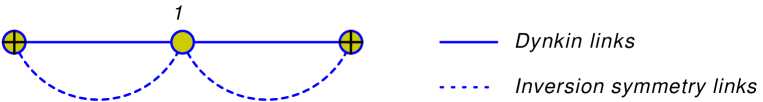
Figure 1: The Dynkin diagram for the Bethe equations. The Dynkin links correspond to the first term in (6.6). The inversion-symmetry links originate from the second term ($A\cdot S$), and in our case are proportional to the Dynkin links.

The equation for the bosonic $\rho_{2}({\tt x})$ density alone (with $\rho_{1}$, $\rho_{3}$ set to zero) describes classical strings on $S^{2}\times\mathbbm{R}_{\rm time}$ [60], as it should.

The finite–gap equations characterize classical solutions of the sigma-model in terms of the spectral data for the Lax operator. The inverse-scattering transformation allows, in principle, to reconstruct any given solution from its spectral data, but for the most part we are interested in the conserved charges that the solution carries, and those can be computed from the quasimomenta.

6.2 Proposal for asymptotic Bethe ansatz equations
for the supercoset sector of states

We can now quantize the above classical Bethe equations using the rules of [56, 57], formulated for general $\mathbbm{Z}_{4}$–cosets in [33]. In quantum theory, the cuts are composed of discrete Bethe roots, that satisfy a set of functional equations, the Bethe equations. The finite-gap equations constitute their classical limit, in the situation when the number of roots is large, and the distance between nearby roots is small such that their distribution can be characterized by a continuous density.

For strings in $AdS_{5}\times S^{5}$, it was possible to reconstruct the quantum Bethe equations from their classical counterpart with the help of extra information from the underlying spin chain [57]. The same approach worked also for the $AdS_{4}\times CP^{3}$ background [58]. In the present case the spin chain description of the dual CFT is not known, but one may observe that the set of rules to convert classical finite–gap equations to quantum Bethe equations follows a uniform model-independent pattern. The same pattern arises in the case at hand, since the structural elements that appear in the finite-gap equations are similar. We may thus apply the same set of rules to convert the classical finite-gap equations into the quantum Bethe equations.

The basic variable of quantum Bethe ansatz is the rapidity $u$, which is related to the spectral parameter by the Zhukowsky transformation

$${\tt x}+\frac{1}{{\tt x}}=u.$$ (6.11)

The dependence on the sigma-model coupling enters through the shifted variables

$${\tt x}^{\pm}+\frac{1}{{\tt x}^{\pm}}=u\pm i\hbar,$$ (6.12)

where “the Planck constant” $\hbar$ is a function of the sigma-model coupling, $(TR^{2})^{-1}=\frac{2\pi\alpha^{\prime}}{R^{2}}$ (with $R$ being the AdS radius) which is not determined by the integrability of the model; we can only say that $\hbar$ coincides with the coupling up to possible higher–order $\alpha^{\prime}$ corrections, i.e. $\hbar={2\pi\alpha^{\prime}\over R^{2}}+O(\alpha^{\prime 2})$.

The Zhukowsky variables determine the momentum and energy of a single worldsheet excitation:

$$\,{\rm e}\,^{i\hbar p}=\frac{{\tt x}^{+}}{{\tt x}^{-}}\,,\qquad\hbar\varepsilon=\frac{i}{{\tt x}^{+}}-\frac{i}{{\tt x}^{-}}+1.$$ (6.13)

The rapidities of individual excitations in a multiparticle state satisfy a set of Bethe equations:

$$1 = \prod_{k}\frac{{\tt x}_{1,j}-{\tt x}_{2,k}^{+}}{{\tt x}_{1,j}-{\tt x}_{2,k}^{-}}\,\,\frac{1-\frac{1}{{\tt x}_{1,j}{\tt x}_{2,k}^{-}}}{1-\frac{1}{{\tt x}_{1,j}{\tt x}_{2,k}^{+}}}\ ,$$

$$\left(\frac{{\tt x}_{j,2}^{+}}{{\tt x}_{j,2}^{-}}\right)^{L} = \prod_{k\neq j}\frac{{\tt x}^{+}_{j,2}-{\tt x}^{-}_{k,2}}{{\tt x}^{-}_{j,2}-{\tt x}^{+}_{k,2}}\,\,\frac{1-\frac{1}{{\tt x}^{+}_{j,2}{\tt x}^{-}_{k,2}}}{1-\frac{1}{{\tt x}^{-}_{j,2}{\tt x}^{+}_{k,2}}}\,\sigma^{4}_{\rm BES}(u_{j,2},u_{k,2})$$

$$\times\prod_{k}\frac{{\tt x}^{-}_{2,j}-{\tt x}_{1,k}}{{\tt x}^{+}_{2,j}-{\tt x}_{1,k}}\,\,\frac{1-\frac{1}{{\tt x}^{+}_{2,j}{\tt x}_{1,k}}}{1-\frac{1}{{\tt x}^{-}_{2,j}{\tt x}_{1,k}}}\,\prod_{k}\frac{{\tt x}^{-}_{2,j}-{\tt x}_{3,k}}{{\tt x}^{+}_{2,j}-{\tt x}_{3,k}}\,\,\frac{1-\frac{1}{{\tt x}^{+}_{2,j}{\tt x}_{3,k}}}{1-\frac{1}{{\tt x}^{-}_{2,j}{\tt x}_{3,k}}}\ ,$$

$$1 = \prod_{k}\frac{{\tt x}_{3,j}-{\tt x}_{2,k}^{+}}{{\tt x}_{3,j}-{\tt x}_{2,k}^{-}}\,\,\frac{1-\frac{1}{{\tt x}_{3,j}{\tt x}_{2,k}^{-}}}{1-\frac{1}{{\tt x}_{3,j}{\tt x}_{2,k}^{+}}}\ .$$ (6.14)

The BES/BHL scattering phase $\sigma_{\rm BES}(u,v)$ [61, 62] (see [63] for a review) is a fairly complicated function of the rapidities. It admits the following integral representation [64]:

$$\sigma_{\rm BES}(u,v) = \exp\left(-i\sum_{r,s=\pm}\chi({\tt x}^{r},{\tt y}^{s})\right),$$

$$\chi({\tt x},{\tt y}) = \frac{i}{4\pi^{2}}\oint_{|z|=1,|w|=1}\frac{dz\,dw}{({\tt x}-z)({\tt y}-w)}\,\,\ln\frac{\Gamma\left(1+\frac{i}{2\hbar}\left(z+\frac{1}{z}-w-\frac{1}{w}\right)\right)}{\Gamma\left(1-\frac{i}{2\hbar}\left(z+\frac{1}{z}-w-\frac{1}{w}\right)\right)}\,.$$ (6.15)

The above Bethe equations are supposed to describe the spectrum of the string in the light-cone gauge defined by the geodesic of a massless particle spinning around $S^{2}$. The parameter $L$ that enters the left-hand-side of the equations is the angular momentum of the ground state ($L=J$). Once ${\tt x}^{\pm}_{2,k}$ are determined, the light-cone energy of the string states for a given collection of Bethe roots is computed by

$$E=\frac{1}{\hbar}\sum_{k}\left(\frac{i}{{\tt x}_{2,k}^{+}}-\frac{i}{{\tt x}_{2,k}^{-}}+1\right).$$ (6.16)

The physical states should satisfy the level matching (zero-momentum) condition:

$$\prod_{k}\frac{{\tt x}_{2,k}^{+}}{{\tt x}_{2,k}^{-}}=\,{\rm e}\,^{i\hbar P_{\rm tot}}\equiv 1.$$ (6.17)

Only the roots on the middle node of the Dynkin diagram ($u_{2}$ roots) carry energy and momentum. The other two types of roots are auxiliary. They just change the flavor composition of the state. These roots are fermionic in the sense that adding an odd number of $u_{1}$ and $u_{3}$ roots produces a fermion.

We should stress that the above Bethe ansatz equations have not been derived from first principles but rather conjectured, building upon structural analogy with other AdS backgrounds. It is a straightforward, albeit lengthy, exercise to show that in the classical limit $\hbar\rightarrow 0$, the quantum Bethe equations (6.2) reduce to the classical finite-gap equations (6.1), with the densities defined by

$$\rho_{l}({\tt x})=2\hbar\sum_{k}\frac{{\tt x}_{l,k}^{2}}{{\tt x}_{l,k}^{2}-1}\,\delta\left({\tt x}-{\tt x}_{l,k}\right).$$ (6.18)

Hence the conjectured equations correctly capture the classical spectrum of the string (this however by construction). It would be important to test them beyond the classical approximation.

Let us check that the Bethe equations (6.2) reproduce the BMN spectrum from sec. 5.1. Their simplest solution is a solitary $u_{2}$ root. According to (6.16), (6.17) and (6.12), at $\hbar\rightarrow 0$ it describes a worldsheet excitation with the momentum and energy

$$p=\frac{2{\tt x}_{2}}{{\tt x}^{2}_{2}-1}\,,\qquad\varepsilon=\frac{{\tt x}^{2}_{2}+1}{{\tt x}^{2}_{2}-1}\,,$$ (6.19)

which in fact parameterize the dispersion relation of a relativistic particle with mass $m^{2}=1$. The Bethe equations reduce to the quantization condition for the momentum: $p=2\pi n/\hbar L$. This is consistent with the light-cone quantization, in which the length of the string is given by its centre-of-mass momentum in the target space: ${\rm Length}=2\pi\alpha^{\prime}L/R^{2}=L\hbar$.

The Bethe equations admit solutions with the $u_{1}$ and/or $u_{3}$ roots added to the solitary $u_{2}$ root. The Bethe equations determine the positions of the auxiliary roots:

$${\tt x}_{1,3}=\frac{{\tt x}_{2}^{+}+{\tt x}_{2}^{-}}{{\tt x}_{2}^{+}{\tt x}_{2}^{-}+1}\approx\frac{2{\tt x}_{2}}{{\tt x}^{2}_{2}+1}\,.$$ (6.20)

These roots change the quantum numbers of the string state without changing its energy. The $1-2$ and $2-3$ complexes are fermions and the $1-2-3$ complex is a boson. The single type–2 root describes the transverse mode of the string on $S^{2}$, the $1-2-3$ stack describes the $AdS_{2}$ mode, and the two fermionic solutions correspond to the two coset fermions that survive the kappa-symmetry gauge fixing. We thus reconstruct the $2_{b}+2_{f}$ massive BMN modes but are obviously missing the $6_{b}+6_{f}$ massless modes, which correspond to the string fluctuations in the $T^{6}$ directions and their superpartners. At the moment we do not understand how to include these modes in the Bethe ansatz framework.

7 Remarks on semiclassical strings in $AdS_{2}\times S^{2}\times T^{6}$

As in the $AdS_{5}\times S^{5}$ case, one may try to check the above Bethe–ansatz based solution for the string spectrum against direct superstring predictions in the limit of large (semiclassical) values of charges.

Already at the string tree level one may compare the corresponding (Landau–Lifshitz–type) effective action following, for coherent states, from the “one-loop” spin chain Hamiltonian formally associated to the Bethe ansatz in (6.2) to the corresponding “fast-string” ($J\gg 1$) limit of the string action. The two are known to match [65] in the $AdS_{5}\times S^{5}$ case due to a special non-renormalization property of the leading order correction in the large $J$ limit.

For example, let us consider classical strings moving in the $S^{2}$ subspace. Following the discussion in Section 5.2 of [66] and eliminating “fast” angular coordinates from the phase-space string action on $R_{t}\times S^{2}$ one finds that it reduces to the same Landau–Lifshitz model that is found, [65], for “slow” coordinates of a fast-moving string in $R\times S^{3}$. In the $R_{t}\times S^{2}$ case, however, the two degrees of freedom are the coordinate and momentum of the “slow” degree of freedom of $S^{2}$. The same action is known also to emerge from the ferromagnetic XXX_1/2 spin chain Hamiltonian (the 1–loop Hamiltonian in the $su(2)$ sector of $\cal N$=4 SYM theory).

This coincidence is, in fact, in agreement with the structure of the Bethe ansatz proposed in the previous section: In the formal weak–coupling limit ($\hbar={2\pi\alpha^{\prime}\over R^{2}}+...\to\infty)$ the central–node part of the Bethe equations (6.2) takes the same form as for the $su(2)$ Heisenberg spin chain (or rather $SO(3)$ subsector of the one-loop $SO(6)$ spin chain): $u_{j}$ and ${\rm x}_{j}$ are then of order $\hbar$, ${\rm x}^{\pm}_{j}=u_{j}\pm i\hbar$, the BES phase disappears, and only the first term on the r.h.s. of the second equation in (6.2) contributes. This implies that the same Landau-Lifshitz model should indeed emerge as a description of the coherent long-wave-length spin-wave states.

At the one-loop string level one may carry out a comparison between the string theory predictions for the 1-loop corrections to energies of semiclassical strings moving in the $AdS_{2}\times S^{2}$ part and the predictions of the Bethe ansatz equations (6.2). One may attempt to do this in general following the approach used in the $AdS_{5}\times S^{5}$ and $AdS_{4}\times CP^{3}$ cases [67, 68, 69]. This should provide, in particular, a check of the BES phase factor in (6.2).

It is useful also to look at specific examples of semiclassical quantization of the simplest string solutions. Let us consider strings moving only in the $AdS_{2}\times S^{2}$ part with the metric given in (5.3). The corresponding classical solutions can be reconstructed, via Pohlmeyer reduction [29, 70], from solutions of the $N=2$ supersymmetric sine-Gordon theory (whose bosonic part is the direct sum of the sine-Gordon and sinh-Gordon models). The standard “vacuum” (BMN) solution, i.e. the massless geodesic wrapping a big circle of $S^{2}$ is $t=\varphi=\nu\tau$,  $\nu={J\over TR^{2}},\ E=J$. It leads (as discussed in Section 5.1) to the small–fluctuation spectrum containing 2 massive ($m=\nu$) bosonic modes, 2 massive fermionic modes and 6+6 massless modes.

In $AdS_{2}\times S^{2}$ there is no place for rigid circular string solutions described by rational functions so the next class of solutions in terms of simplicity are rigid spinning or pulsating strings described by elliptic functions. One example is the giant magnon [71] (an open string spinning in $S^{2}$ with its ends on a big circle) which of course has the same classical dispersion relation as in the $AdS_{5}\times S^{5}$ case. The corresponding small fluctuation spectrum can be analysed as in [72, 73], now starting with the $AdS_{2}\times S^{2}\times T^{6}$ superstring action. Instead of 4 massive bosonic fluctuations from $AdS_{5}$ one finds one from $AdS_{2}$ with the same stability angle $\nu_{1}$; instead of 4 bosonic fluctuations from $S^{5}$ one gets 1 from $S^{2}$ with the same stability angle $\nu_{2}=\nu_{1}+2{\rm arccot}\ k$ (where $k$ is the spatial 2d momentum number); instead of 8 massive fermionic modes one gets 2 massive fermions from the supercoset part of the action with $\nu_{3}=\nu_{1}+{\rm arccot}\ k$. In addition, there are 6 decoupled massless $T^{6}$ modes and 6 massless fermions (after $\kappa$-gauge fixing). The “non-coset” fermions do not get mass from the RR coupling term in the quadratic fermionic action (due to the structure of the projector in (3.4) or (3.19)) while the induced connection term in the covariant derivative (2.2) can be rotated away. As a result, the 1-loop correction to the string energy (determined by $\nu_{1}+\nu_{2}-2\nu_{3}$) vanishes as in the $AdS_{5}\times S^{5}$ case [73].

Another simple elliptic solution is a folded string rotating around its center of mass in $S^{2}$ [74]:

$$t=\kappa\tau,\ \ \ \theta=\theta(\sigma),\ \ \ \varphi=w\tau,\ \ \ \ \ \theta^{\prime 2}=\kappa^{2}-w^{2}\sin^{2}\theta\ ,$$ (7.1)

$$\sin\theta=\sqrt{q}\ {\rm sn}(w\sigma|q)\ ,\ \ \ \ q=\sin^{2}\theta_{0}={\kappa^{2}\over w^{2}}\ ,\ \ \ \ w={2\over\pi}{\rm K}(q)\ ,$$ (7.2)

where ${\rm K}$ is the elliptic integral. In the case of $AdS_{n}\times S^{n}\times T^{10-2n}$ (with $n=5,3,2$) the corresponding quadratic fluctuation spectrum can be found by imposing the static gauge on the fluctuations and turns out to be a simple truncation of the $AdS_{5}\times S^{5}$ spectrum found in [75]. It is described by a combination of massive bosonic and fermionic 2d modes with the following degeneracy $\times$ (mass)²

$${\rm Bosons}:\ \ \ \ AdS_{n}:\ \ \ (n-1)\times\kappa^{2};$$

$$\ \ \ \ \ \ \ \ \ \ \ \ \ \ \ \ \ \ S^{n}:\ \ \ 1\times\kappa^{2}[1-{2(\kappa^{2}-w^{2})\over\kappa^{2}-w^{2}\sin^{2}\theta}];\ \ (n-2)\times(2w^{2}\sin^{2}\theta-\kappa^{2})$$

$$\ \ \ \ \ \ \ \ \ \ \ \ \ \ \ \ \ \ \ T^{10-2n}:\ \ \ (10-2n)\times 0$$

$${\rm Fermions}:\ \ \ \ 2(n-1)\times w^{2}\sin^{2}\theta;\ \ (10-2n)\times 0\ .$$ (7.3)

The resulting mass sum rule that checks the 1-loop UV finiteness of the GS string in the static gauge is then universal in $n$ (see [75])

$$\sum(m^{2}_{B}-m^{2}_{F})=2\Big{(}\kappa^{2}-w^{2}\sin^{2}\theta-\kappa^{2}{\kappa^{2}-w^{2}\over\kappa^{2}-w^{2}\sin^{2}\theta}\Big{)}=\sqrt{-g}R^{(2)}\ .$$ (7.4)

Here the coset part decouples from the torus part of the model. This is due, in particular, to the possibility of rotating away the connection in the covariant derivative in the fermionic part, i.e. the masses come solely from the RR flux term coupling in the quadratic fermionic action. The resulting 1-loop correction to the folded string energy in $AdS_{2}\times S^{2}\times T^{6}$ can be computed by direct combination of the expressions given in [75].

A similar analysis can be carried out for the circular pulsating solution on $S^{2}$ [76] which is described in conformal gauge by (cf. (7.2))

$$t=\kappa\tau,\ \ \ \theta=\theta(\tau),\ \ \ \varphi=m\sigma,\ \ \ \ \ \dot{\theta}^{2}=\kappa^{2}-w^{2}\sin^{2}\theta\ ,$$ (7.5)

$$\sin\theta=\sqrt{q}\ {\rm sn}(m\tau|q)\ ,\ \ \ \ \ \ \ q=\sin^{2}\theta_{0}={\kappa^{2}\over m^{2}}\ ,\ \ \ \ \ \ w={2\over\pi}{\rm K}({\kappa\over w})\ .$$ (7.6)

For a superstring in $AdS_{n}\times S^{n}\times T^{10-2n}$ ($n=5,3,2$) the corresponding quadratic fluctuation spectrum in the static gauge is again a truncation of the $AdS_{5}\times S^{5}$ spectrum in [75]:

$${\rm Bosons}:\ \ \ \ AdS_{n}:\ \ \ (n-1)\times\kappa^{2};$$

$$\ \ \ \ \ \ \ \ \ \ \ \ \ \ \ \ \ \ S^{n}:\ \ \ 1\times\kappa^{2}(1-{2\over\sin^{2}\theta});\ \ \ (n-2)\times(\kappa^{2}-2m^{2}\sin^{2}\theta)$$

$$\ \ \ \ \ \ \ \ \ \ \ \ \ \ \ \ \ \ \ T^{10-2n}:\ \ \ (10-2n)\times 0$$

$${\rm Fermions}:\ \ \ \ 2(n-1)\times(\kappa^{2}-m^{2}\sin^{2}\theta);\ \ \ (10-2n)\times 0\ .$$ (7.7)

Again, we get a universal mass sum rule that checks the UV finiteness (see [75])

$$\sum(m^{2}_{B}-m^{2}_{F})=2\Big{(}m^{2}-{\kappa^{2}\over\sin^{2}\theta}\Big{)}=\sqrt{-g}R^{(2)}\,.$$ (7.8)

As in the previous examples, the masses come only from the RR coupling term and the toroidal part decouples and does not contribute to the 1–loop correction to the string energy.

Given that the Bethe ansatz equations (6.2) were constructed on the basis of the supercoset part of the string model (i.e. under the assumption of the decoupling of the non–supercoset parts) this guarantees the agreement between their predictions and the direct superstring predictions for the 1–loop energies of the above solutions. This agreement should also extend to the leading strong coupling finite size (TBA) generalization of the asymptotic Bethe ansatz equations as there should be a direct analog of the analysis in [77]. One may also hope that higher order (2-loop, etc.) string corrections to energies of semiclassical string solutions in $AdS_{2}\times S^{2}$ will not be sensitive to contributions of massless toroidal modes. A priori, this may not apply to the full quantum string spectrum which may be sensitive to finite-size corrections due to massless modes.

Let us now comment on the case of semiclassical strings moving also in the toroidal part. In general, the radii ${\rm r}_{i}$ of $T^{6}$ (or, more generally, its constant metric) are free parameters of the model, in addition to the radius ${R}$ of $AdS_{2}$ and $S^{2}$. Thus by varying ${\rm r}_{i}/{R}$ we may suppress or enhance the contributions of configurations in which the string is moving in $T^{6}$. For example, we may generalize the above solutions to the case when the c.o.m. of the string moves in $S^{1}$ of $T^{6}$,  $y\equiv{\rm r}\psi,\ \psi=p\tau,\ \ P={r^{2}\over\alpha^{\prime}}p.$ That will generalize the energy relation $E=J$ we had for the BMN state in $S^{2}$ as follows:

$$\kappa^{2}=\nu^{2}+\gamma^{2}p^{2},\ \ \ \ {\rm i.e.}\ \ \ \ E^{2}=J^{2}+\gamma^{-2}P^{2},\ \ \ \ \ \ \gamma\equiv{{{\rm r}}\over{R}}\ .$$ (7.9)

The corresponding fluctuation spectrum was already discussed in Section 5.2. While the bosonic modes from $T^{6}$ remain massless 2 of the non–supercoset–like fermions $\upsilon^{\prime}$ get non–zero mass, i.e. the coset and non–coset sectors no longer decouple.

This non–decoupling will happen also for extended string solutions, e.g., a simple circular spinning string solution constructed by allowing the string to wind around a big circle of $S^{2}$ as well as around a circle in $T^{6}$ ($n$ and $k$ are integer winding numbers)

$$t=\kappa\tau\ ,\ \ \theta={\pi\over 2}\ ,\ \ \ \varphi=w\tau+n\sigma,\ \ \ \ \ \ \psi=p\tau-k\sigma\ ,$$

$$\kappa^{2}=w^{2}+n^{2}+\gamma^{2}(p^{2}+k^{2})\ ,\ \ \ \ \ wm=\gamma^{2}pk\ .$$ (7.10)

Here again the non-coset fermions will get non-trivial masses and give a non-trivial contribution to the 1-loop correction to the energy.

Imposing the conformal gauge, the general $T^{6}$ solution can be written as $y_{m^{\prime}}=u_{m^{\prime}}(\sigma_{+})+\tilde{u}_{m^{\prime}}(\sigma_{-}),\ \ \sigma_{\pm}=\sigma\pm\tau$, so that $T_{++}(T^{6})=u^{\prime 2}(\sigma_{+}),\ T_{--}(T^{6})=\tilde{u}^{\prime 2}(\sigma_{-})$. We may fix the residual conformal diffeomorphisms by assuming that $T_{++}(AdS_{2})=T_{--}(AdS_{2})=-\mu^{2}=$const. Then the Virasoro conditions $T^{(tot)}_{\pm\pm}=0$ imply that

$$T_{++}(S^{2})=(\mu^{2}-u^{\prime 2})\equiv h^{2}(\sigma_{+})\ ,\ \ \ \ \ \ \ T_{--}(S^{2})=(\mu^{2}-\tilde{u}^{\prime 2})\equiv\tilde{h}^{2}(\sigma_{-})\ .$$ (7.11)

Since the $T_{\pm\pm}(S^{2})$ components are now non-constant, as was already mentioned in Section 6, in the case when the string moves in $T^{6}$ one cannot describe the corresponding $AdS_{2}\times S^{2}\times T^{6}$ solutions using the finite gap construction.

Let us mention that a related problem appears also when one tries to apply the Pohlmeyer reduction approach to describe such string solutions. Instead of the sinh-Gordon theory plus the standard sine-Gordon theory as found in the $AdS_{2}\times S^{2}$ case one now ends up with

$$L=\partial_{+}\chi\partial_{-}\chi-{\mu^{2}\over 2}\cosh 2\chi+\partial_{+}\varphi\partial_{-}\varphi+{1\over 2}h(\sigma_{+})\tilde{h}(\sigma_{-})\cos 2\varphi\ .$$ (7.12)

In the equation for $\varphi$ one can formally replace $h(\sigma_{+})\tilde{h}(\sigma_{-})$ by a constant performing a conformal redefinition of $\sigma_{\pm}$. The result will be the sine–Gordon equation on a complicated 2d domain, determined by functions that parameterize the $T^{6}$ solution.

8 Conclusion

In this paper we considered GS superstrings in $AdS_{2}\times S^{2}\times T^{6}$ backgrounds that represent consistent embeddings of $AdS_{2}\times S^{2}$ space-time into critical string theory. We have shown that the full 10d structure of the superstring theory cannot be captured just by its effective $AdS_{2}\times S^{2}$ “supercoset” part described by an integrable sigma–model on $PSU(1,1|2)/SO(1,1)\times U(1)$, though the latter is, indeed, a consistent classical truncation of the full theory. Nevertheless, we have provided direct evidence for the classical integrability of the complete theory by constructing the Lax representation of its equations of motion to the second order in fermions.

In general, the $T^{6}$ sector does not decouple from the $AdS_{2}\times S^{2}$ one due to non-zero RR flux components along the $T^{6}$ directions which couple derivatives of the $T^{6}$ coordinates to the GS fermions. We illustrated this in the example of the second BMN limit in Section 5.2. Still, for strings moving only in the $AdS_{2}\times S^{2}$ subspace the decoupling does take place at the one-loop level (Section 7) and that may extend to all orders in the semiclassical (large-charge) expansion.

For the part of the string spectrum which is associated with the supercoset sector we have proposed Bethe equations that are of the asymptotic Bethe ansatz type. They are supposed to describe quantum states with sufficiently large quantum numbers up to exponential corrections. In other words, they describe the string sigma–model on an infinite plane rather than on a cylinder (the length of the string in the light-cone gauge is proportional to its light–cone momentum, and if the light–cone momentum is large, the internal length of the string goes to infinity). Application of a more general TBA or Y–system framework (see [78] for a review) to this theory will likely require understanding the massless $T^{6}$ modes and the non–coset fermionic excitations of the string that we have ignored in our analysis of the Bethe equations.

The super $AdS_{2}\times S^{2}$ background is one of the few GS–type cosets, which are simultaneously integrable and conformal. Other possible candidates that contain an $AdS_{2}$ factor are $AdS_{2}\times S^{2}\times S^{2}$ and $AdS_{2}\times S^{3}$ [30]. It would be interesting to find critical string backgrounds which contain these cosets as consistent truncations. It would be also of interest to verify if the fermionic T-duality of the supercoset model [26] persists in the presence of the non-supercoset fermions.

Appendix A. Main notation and conventions

We assume the metric to have the ‘almost plus’ signature $(-,+,\cdots,+)$. Generically, the tangent space vector indices are labeled by letters from the beginning of the Latin alphabet, while letters from the middle of the Latin alphabet stand for curved (world) indices. The spinor indices are labeled by Greek letters. The direct product $AdS_{2}\times S^{2}\times T^{6}$ is parametrized, respectively, by the coordinates $x^{m}$ $(m=0,1)$, $x^{\hat{m}}$ $(\hat{m}=2,3)$ and $y^{m^{\prime}}$ $(m^{\prime}=4,5,6,7,8,9)$. Its vielbeins are, respectively, $e^{a}=dx^{m}\,e_{m}{}^{a}(x)$ (${a}=0,1$), $e^{\hat{a}}=dx^{\hat{m}}\,e_{\hat{m}}{}^{\hat{a}}(\hat{x})$ (${\hat{a}}=2,3$) and $e^{a^{\prime}}(y)=dy^{a^{\prime}}$. The $AdS_{2}$ curvature is

$$R_{abc}{}^{d}=\frac{2}{R^{2}}\,\eta_{c[a}\,\delta_{b]}^{d}\,,\qquad R^{ab}=-\frac{1}{R^{2}}\,e^{a}\,e^{b}\,,$$ (A.1)

where ${R}$ is the $AdS_{2}$ radius, and the $S^{2}$ curvature is

$$R_{\hat{a}\hat{b}\hat{c}}{}^{\hat{d}}=-\frac{2}{R^{2}}\,\eta_{\hat{c}[\hat{a}}\,\delta_{\hat{b}]}^{\hat{d}}\,,\qquad R^{\hat{a}\hat{b}}=\frac{1}{R^{2}}\,e^{\hat{a}}\,e^{\hat{b}}\,.$$ (A.2)

The $D=4$ gamma–matrices in $AdS_{2}\times S^{2}$ are

$$\{\gamma^{\underline{a}},\gamma^{\underline{b}}\}=2\,\eta^{\underline{ab}}\,,\qquad\eta^{\underline{ab}}={\rm diag}\,(-,+,+,+)\,,\qquad\underline{a}=(a,\hat{a})$$ (A.3)

$$\gamma^{5}=i\gamma^{0}\,\gamma^{1}\,\gamma^{2}\,\gamma^{3},\qquad\gamma^{5}\,\gamma^{5}=1\,.$$ (A.4)

The charge conjugation matrix $C$ is antisymmetric, the matrices $(\gamma^{\underline{a}})_{\alpha\beta}\equiv(C\,\gamma^{\underline{a}})_{\alpha\beta}$ and $(\gamma^{\underline{ab}})_{\alpha\beta}\equiv(C\,\gamma^{\underline{ab}})_{\alpha\beta}$ are symmetric and $\gamma^{5}_{\alpha\beta}\equiv(C\gamma^{5})_{\alpha\beta}$ is antisymmetric, with $\alpha,\beta=1,2,3,4$ being the indices of a 4–dimensional spinor representation of $SO(1,3)$. These $4\times 4$ matrices can be represented in terms of $2\times 2$ $AdS_{2}$ gamma–matrices $\rho^{a}$ ($a=0,1$) and the matrices $\rho^{\hat{a}}$ ($\rho^{2}=\sigma^{1}$, $\rho^{3}=\sigma^{3}$) associated with $S^{2}$ as

$$\gamma^{a}=\rho^{a}\otimes\mathbf{1},\qquad\gamma^{\hat{a}}=\gamma\otimes\rho^{\hat{a}}\,,\qquad\gamma=\rho^{0}\rho^{1}\,.$$ (A.5)

$8\times 8$ gamma–matrices associated with $T^{6}$ are

$$\{\gamma^{a^{\prime}},\gamma^{b^{\prime}}\}=2\,\delta^{{a^{\prime}}{b^{\prime}}}\,,\qquad\delta^{a^{\prime}b^{\prime}}={\rm diag}\,(+,+,+,+,+,+)\,,$$ (A.6)

$$\gamma^{7}={i\over{6!}}\,\varepsilon_{\,a_{1}^{\prime}a_{2}^{\prime}a_{3}^{\prime}a_{4}^{\prime}a_{5}^{\prime}a_{6}^{\prime}}\,\gamma^{a_{1}^{\prime}}\cdots\gamma^{a_{6}^{\prime}}\qquad\gamma^{7}\,\gamma^{7}=1\,.$$ (A.7)

The charge conjugation matrix $C^{\prime}$ is symmetric and the matrices $(\gamma^{a^{\prime}})_{\alpha^{\prime}\beta^{\prime}}\equiv(C^{\prime}\,\gamma^{a^{\prime}})_{\alpha^{\prime}\beta^{\prime}}$ and $(\gamma^{a^{\prime}b^{\prime}})_{\alpha^{\prime}\beta^{\prime}}\equiv(C^{\prime}\,\gamma^{a^{\prime}b^{\prime}})_{\alpha^{\prime}\beta^{\prime}}$ are antisymmetric, with $\alpha^{\prime},\beta^{\prime}=1,\cdots,8$ being the indices of an 8–dimensional spinor representation of $SO(6)$.

Using the matrices (A.3) and (A.6) one can construct the $D=10$ gamma–matrices $\Gamma^{A}$ as

$$\{\Gamma^{A},\,\Gamma^{B}\}=2\eta^{AB},\qquad\Gamma^{A}=(\Gamma^{\underline{a}},\,\Gamma^{a^{\prime}})\,,$$ (A.8)

$$\Gamma^{\underline{a}}=\gamma^{\underline{a}}\,\otimes\,{\bf 1},\qquad\Gamma^{a^{\prime}}=\gamma^{5}\,\otimes\,\gamma^{a^{\prime}},\qquad\Gamma^{11}=\gamma^{5}\,\otimes\,\gamma^{7},\qquad\underline{a}=0,1,2,3;\quad a^{\prime}=4,\cdots,9\,.$$

The charge conjugation matrix is ${\mathcal{C}}=C\otimes C^{\prime}$. In this realization the 32–component spinor $\Theta^{\alpha\alpha^{\prime}}$ is labelled by the 4–component $AdS_{2}\times S^{2}$ spinor index $\alpha$ and the 8–component $T^{6}$ spinor index $\alpha^{\prime}$.

Finally we can introduce a spinor projection operator which projects onto an 8-dimensional subspace of the 32-dimensional space of spinors as follows

$$\mathcal{P}_{8}=\frac{1}{8}(2-iJ_{a^{\prime}b^{\prime}}\Gamma^{a^{\prime}b^{\prime}}\gamma^{7})\,,$$ (A.9)

where $J_{a^{\prime}b^{\prime}}$ is the Kähler form on $T^{6}$.

Appendix B. Enlarged $\mathfrak{psu}(1,1|2)$ superalgebra

The $\mathfrak{psu}(1,1|2)$ superalgebra has the following conventional form. Its bosonic $SO(2,1)\times SO(3)$ subalgebra is generated by translations $P_{\underline{a}}=(P_{a},P_{\hat{a}})$ and $SO(1,1)\times SO(2)$ rotations $M_{\underline{ab}}=(M_{ab},M_{\hat{a}\hat{b}})$ in $AdS_{2}\times S^{2}$

$$[P_{\underline{a}},P_{\underline{b}}]=-\frac{1}{2}R_{{\underline{a}}{\underline{b}}}{}^{{\underline{c}}{\underline{d}}}\,M_{{\underline{c}}{\underline{d}}}\,,\qquad[M_{{\underline{a}}{\underline{b}}},P_{\underline{c}}]=\eta_{{\underline{a}}{\underline{c}}}P_{\underline{b}}-\eta_{{\underline{b}}{\underline{c}}}P_{\underline{a}},$$

$${}[M_{{\underline{a}}{\underline{b}}},M_{{\underline{c}}{\underline{d}}}]=\eta_{{\underline{a}}{\underline{c}}}M_{{\underline{b}}{\underline{d}}}+\eta_{{\underline{b}}{\underline{d}}}M_{{\underline{a}}{\underline{c}}}-\eta_{{\underline{b}}{\underline{c}}}M_{{\underline{a}}{\underline{d}}}-\eta_{{\underline{a}}{\underline{d}}}M_{{\underline{b}}{\underline{c}}}\,,$$ (B.1)

where

$$R_{\underline{ab}}{}^{\underline{cd}}=(R_{ab}{}^{cd},R_{\hat{a}\hat{b}}{}^{\hat{c}\hat{d}})=(\frac{2}{R^{2}}\delta_{[a}^{c}\delta_{b]}^{d},-\frac{2}{R^{2}}\delta_{[\hat{a}}^{\hat{c}}\delta_{\hat{b}]}^{\hat{d}})$$ (B.2)

is the $AdS_{2}\times S^{2}$ curvature. The fermionic part of $PSU(1,1|2)$ is generated by eight Grassmann–odd operators $Q_{\alpha I}$ carrying the index $\alpha=1,2,3,4$ of a spinorial representation of $SO(1,1)\times SO(2)$ and the vector index $I=1,2$ of the group $SO(2)$ of external automorphisms of $PSU(1,1|2)$. The generators $Q$ satisfy the following (anti)commutation relations

$$[P_{\underline{a}},Q_{I}]=\frac{1}{2R}\varepsilon_{IJ}\,Q_{J}\gamma\gamma_{\underline{a}}\,,\qquad[M_{{\underline{a}}{\underline{b}}},Q]=-\frac{1}{2}Q\gamma_{{\underline{a}}{\underline{b}}}\,,\qquad[{\rm T},Q_{I}]=\frac{1}{2}\,\varepsilon_{IJ}\,Q_{J}\,,$$ (B.3)

$$\{Q_{I},Q_{J}\}=2i\,\delta_{IJ}\,\gamma^{\underline{a}}\,P_{\underline{a}}+\frac{iR}{2}\varepsilon_{IJ}\,\gamma^{{\underline{a}}{\underline{b}}}\,\gamma\,R_{{\underline{a}}{\underline{b}}}{}^{{\underline{c}}{\underline{d}}}M_{{\underline{c}}{\underline{d}}}\,,$$ (B.4)

where the spinorial indices are suppressed, $\gamma^{\underline{a}}$ and $\gamma=\gamma^{0}\gamma^{1}$ are the $D=4$ gamma matrices with $AdS_{2}\times S^{2}$ indices and ${\rm T}$ is the generator of the external $SO(2)$ automorphism of $PSU(1,1|2)$. As we will see below, from a ten-dimensional point of view it is natural to include ${\rm T}$, even though it is not an element of $\mathfrak{psu}(1,1|2)$.

Since the GS formulation of the string in $AdS_{2}\times S^{2}\times T^{6}$ uses, a priori, $D=10$ notation and 32–component spinors, we have found it convenient to formally lift the $\mathfrak{psu}(1,1|2)$ superalgebra to ten dimensions and enlarge it with additional generators $P_{a^{\prime}}$ and $M_{a^{\prime}b^{\prime}}$ of the U(1) isometries and $SO(6)$ rotations in $T^{6}$. The $\mathfrak{psu}(1,1|2)$ superalgebra enlarged in such a way looks very similar to the $OSp(6|4)$ superalgebra in the form used in [32]. This similarity allows us to use the same gamma–matrix identities as those found in [36] for the $AdS_{4}\times CP^{3}$ case.

To rewrite the $\mathfrak{psu}(1,1|2)$ superalgebra in a formally $D=10$ covariant form we replace the $D=4$ gamma–matrices with their $D=10$ counterparts $\Gamma^{A}$ and represent the 8 fermionic generators $Q_{\alpha I}$ as 32–component spinors subject to the 8–dimensional projection

$$Q=\mathcal{P}_{8}\,Q\ ,$$ (B.5)

with $\mathcal{P}_{8}$ having 8 non–zero eigenvalues and satisfying the commutation relations (3.6) and (3.7).

The following reasoning demonstrates the relation between the $\mathcal{P}_{8}$–projected 32–component spinor $Q_{\alpha\alpha^{\prime}}$ with the two 4–component $AdS_{2}\times S^{2}$ spinors $Q_{\alpha I}$. The projector $\mathcal{P}_{8}$ and $\Gamma_{(3)}$, introduced in eq. (3.20), commute and can be simultaneously diagonalized. Because the projector $\mathcal{P}_{8}$ also commutes with the 6d chirality $\gamma^{7}$, while $\Gamma_{(3)}$ anti–commutes with it, the eigenvalues of $\mathcal{P}_{8}$ (in the 6d spinor space) are doubly degenerate, each pair having opposite values of $\Gamma_{(3)}$. On the other hand, $\mathcal{P}_{8}$ and $\Gamma_{(3)}$ commute with $\Gamma^{\underline{a}}$ and thus leave the 4d spinor index $\alpha$ intact. Thus, under the action of $\mathcal{P}_{8}$, the 6d spinor index $\alpha^{\prime}$ then reduces to the binary index $I=1,2$ that labels the eigenvalues of $\Gamma_{(3)}$ and is associated with the $SO(2)$–automorphism.

From the $D=10$ perspective the external $SO(2)$ automorphism of $\mathfrak{psu}(1,1|2)$ becomes an Abelian subgroup of the group $SO(6)$ of rotations of the $T^{6}$–torus associated with the Kähler form $J_{a^{\prime}b^{\prime}}$ on $T^{6}$. Namely, the $SO(2)$ generator ${\rm T}=\frac{1}{6}J^{a^{\prime}b^{\prime}}M_{a^{\prime}b^{\prime}}$ can be regarded as the part of $M_{a^{\prime}b^{\prime}}$ which acts non–trivially on $Q$. Rewriting the commutator $[T,Q]$ of eq. (B.3) in ten–dimensional notation we have

$$[{\rm T},Q]=-\frac{i}{2}Q\gamma^{7}\mathcal{P}_{8}\qquad\Rightarrow\qquad[M_{a^{\prime}b^{\prime}},Q]:=-\frac{i}{2}J_{a^{\prime}b^{\prime}}Q\gamma^{7}\mathcal{P}_{8}=-\frac{1}{2}Q\Gamma_{a^{\prime}b^{\prime}}\mathcal{P}_{8},$$ (B.6)

where

$$\gamma^{7}=i\Gamma^{4}\cdots\Gamma^{9}$$ (B.7)

is the product of the six gamma–matrices with $T^{6}$ indices. In (B.6) we have used the gamma–matrix identities

$$\mathcal{P}_{8}\Gamma_{a^{\prime}b^{\prime}}\mathcal{P}_{8}=iJ^{a^{\prime}b^{\prime}}\gamma^{7}\mathcal{P}_{8},\qquad\gamma^{7}\mathcal{P}_{8}=\mathcal{P}_{8}\gamma^{7}\qquad{\rm and}\qquad\mathcal{P}_{8}\gamma^{7}\mathcal{P}_{8}:=i\varepsilon\otimes\mathbf{1.}$$

The last expression relates the $2\times 2$ antisymmetric matrix $\varepsilon$ of eqs. (B.3) and (B.4) times the unit $4\times 4$ spinor matrix in $AdS_{2}\times S^{2}$ with the $\mathcal{P}_{8}$–projected matrix $\gamma^{7}$, eq. (B.7).

Now, let us note that $Q$ commutes with the generators $P_{a^{\prime}}$ of the $U(1)$ isometries of $T^{6}$. Then, since $\mathcal{P}_{8}\Gamma_{a^{\prime}}\mathcal{P}_{8}\equiv 0$, the zero commutator $[P_{a^{\prime}},Q]$ can be written as

$$[P_{a^{\prime}},Q]=\frac{i}{2R}Q\gamma\gamma^{7}\Gamma_{a^{\prime}}\mathcal{P}_{8}\equiv 0,$$

where now $\gamma=\Gamma^{0}\Gamma^{1}=\gamma^{01}\otimes\mathbf{1}$ is the product of $D=10$ gamma–matrices carrying $AdS_{2}$ indices. Taking all this into account we can write the enlarged $\mathfrak{psu}(1,1|2)$ superalgebra in the following form

$$[P_{A},P_{B}]=-\frac{1}{2}R_{AB}{}^{CD}M_{CD}\,,\qquad[M_{AB},P_{C}]=\eta_{AC}P_{B}-\eta_{BC}P_{A}\,,$$

$$[M_{AB},M_{CD}]=\eta_{AC}M_{BD}+\eta_{BD}M_{AC}-\eta_{BC}M_{AD}-\eta_{AD}M_{BC}\,,$$ (B.8)

$$[P_{A},Q]=\frac{i}{2R}Q\gamma\gamma^{7}\Gamma_{A}\mathcal{P}_{8}\,,\qquad[M_{AB},Q]=-\frac{1}{2}Q\Gamma_{AB}\mathcal{P}_{8}\,,$$

$$\{Q,Q\}=2i(\mathcal{P}_{8}\Gamma^{A}\mathcal{P}_{8})P_{A}+\frac{R}{2}(\mathcal{P}_{8}\Gamma^{AB}\gamma\gamma^{7}\mathcal{P}_{8})R_{AB}{}^{CD}M_{CD}\,,$$ (B.9)

where $M_{AB}=(M_{ab},M_{\hat{a}\hat{b}},M_{a^{\prime}b^{\prime}})$ and $P_{A}=(P_{a},P_{\hat{a}},P_{a^{\prime}})$ are the generators of Lorentz-transformations and translations in $AdS_{2}$, $S^{2}$ and $T^{6}$, respectively, and

$$R_{AB}{}^{CD}=(R_{ab}{}^{cd},R_{\hat{a}\hat{b}}{}^{\hat{c}\hat{d}},0)=(\frac{2}{R^{2}}\delta_{[a}^{c}\delta_{b]}^{d},-\frac{2}{R^{2}}\delta_{[\hat{a}}^{\hat{c}}\delta_{\hat{b}]}^{\hat{d}},0)$$ (B.10)

is the curvature tensor of $AdS_{2}\times S^{2}\times T^{6}$.

To recapitulate, the above form of the $\mathfrak{psu}(1,1|2)$ superalgebra is convenient for our purposes since it is formulated in a $D=10$ covariant way and takes a form very similar to that of $OSp(6|4)$ [36, 32].

Appendix C. Basic relations for the Killing vectors on symmetric spaces $G/H$

Let $K_{M}(X)$ or $K_{A}(X)=e_{A}{}^{M}(X)\,K_{M}(X)$ be the Killing vectors of a $D$–dimensional symmetric space $G/H$, where $M$ are world indices and $A$ are tangent space indices. The Killing vectors $K_{M}(X)$ take values in the algebra of the isometry group $G$ and the one–forms $K=dX^{M}\,K_{M}$ satisfy the Maurer–Cartan equations

$$dK=-2K\wedge K\ ,\qquad dK\wedge K=K\wedge dK=-2K\wedge K\wedge K\ .$$ (C.1)

The following relations also hold

$$[\nabla_{A},\nabla_{B}]K_{C}=-R_{ABC}{}^{D}\,K_{D}\,,\qquad\nabla_{A}K_{B}=[K_{A},K_{B}],\qquad$$

$$\nabla_{A}\nabla_{B}K_{C}=[\nabla_{A}K_{B},\,K_{C}]+[K_{B},\nabla_{A}K_{C}]=[\nabla_{A}K_{B},\,K_{C}]-[\nabla_{A}K_{C},\,K_{B}]=-2R_{A[BC]}{}^{D}K_{D},\,\,\,\,\,\,\,~{}$$

$$\,[\nabla_{A}K_{B},\,K_{C}]=[[K_{A},\,K_{B}],\,K_{C}]=-R_{ABC}{}^{D}\,K_{D},$$

$$\Big{[}[K_{A},K_{B}],[K_{C},K_{D}]\Big{]}=R_{AB[C}{}^{F}\,[K_{D]},K_{F}]-R_{CD[A}{}^{F}\,[K_{B]},K_{F}]\,,$$

where $R_{ABC}{}^{D}$ is the curvature of the symmetric space $G/H$.

Appendix D. Equations of motion from flatness
of the Lax connection

We have seen that the Lax connection defined in (2.15)–(2.19) is indeed flat for the type IIA and IIB superstring on $AdS_{2}\times S^{2}\times T^{6}$ with RR–flux, provided that the equations of motion are satisfied. To have integrability the opposite should also hold, i.e. requiring flatness of the Lax connection should imply the equations of motion for the string. Here we will show that this is indeed the case.

Computing the curvature of the Lax–connection defined in (2.15)–(2.19), (2.21) and (2.25) without using the equations of motion we get

$$dL-LL=\alpha_{2}(\nabla\ast J^{A}-e^{D}\ast J^{BC}R_{BCD}{}^{A})K_{A}-\frac{i}{2}\alpha_{2}(1+\alpha_{1})\Theta\Gamma^{AB}\not{e}\mathcal{D}\Theta\,\nabla_{A}K_{B}$$

$$\ \ \ \ \ +(-1)^{\nu}\frac{i}{2}\alpha_{2}^{2}\Theta\Gamma^{AB}\hat{\Gamma}\not{e}\mathcal{D}\Theta\,\nabla_{A}K_{B}-\frac{i}{2R}\alpha_{2}\beta_{2}\,\Xi\not{e}\mathcal{D}\Theta-(-1)^{\nu}\frac{i}{2R}\alpha_{2}\beta_{1}\,\Xi\hat{\Gamma}\not{e}\mathcal{D}\Theta\,,$$ (D.1)

where $\nu=1(0)$ for type IIA(B) and

$$\not{e}\mathcal{D}\Theta=\ast e^{A}\,\Gamma_{A}\mathcal{D}\Theta-e^{A}\,\Gamma_{A}\hat{\Gamma}\mathcal{D}\Theta$$ (D.2)

is the quantity that is set to zero by the fermionic equations of motion.

Since the coefficients are all independent (they are different functions of the spectral parameter) each term has to vanish separately. The vanishing of the first term implies

$$\nabla(\ast e^{A}+i\Theta\Gamma^{A}\ast E+i\Theta\Gamma^{A}\hat{\Gamma}E-\frac{i}{8}\ast e^{B}\,\Theta\Gamma^{A}\not{F}\Gamma_{B}\Theta-\frac{i}{8}e^{B}\,\Theta\Gamma^{A}\hat{\Gamma}\not{F}\Gamma_{B}\Theta)-e^{D}\ast J^{BC}R_{BCD}{}^{A}=0\,,$$ (D.3)

which, using (2.9), is equal to the bosonic equations of motion (2.5).

The vanishing of the last two terms in the curvature implies the $\mathcal{P}_{8}$ projection of the fermionic equations of motion,

$$\mathcal{P}_{8}\not{e}\mathcal{D}\Theta=0\,.$$ (D.4)

We thus get eight fermionic equations of motion associated with the supercoset fermions $\vartheta$.

To single out the remaining 24 fermionic equations we notice that there are two other terms in (Appendix D. Equations of motion from flatness of the Lax connection) which have to vanish:

$$\Theta\Gamma^{\underline{ab}}\not{e}\mathcal{D}\Theta$$ (D.5)

and

$$\Theta\Gamma^{\underline{ab}}\hat{\Gamma}\not{e}\mathcal{D}\Theta\,,$$ (D.6)

where $(\underline{ab})=(01),(23)$ (note that the covariant derivative of $T^{6}$–translation Killing vectors $\nabla_{a^{\prime}}K_{b^{\prime}}$ vanishes so the corresponding terms are absent). Using the $\mathcal{P}_{8}$ projection of the fermionic equation of motion, which we already found, we get the conditions

$$\upsilon\Gamma^{01}(1-\mathcal{P}_{8})\not{e}\mathcal{D}\Theta=\upsilon\Gamma^{23}(1-\mathcal{P}_{8})\not{e}\mathcal{D}\Theta=\upsilon\Gamma^{01}(1-\mathcal{P}_{8})\hat{\Gamma}\not{e}\mathcal{D}\Theta=\upsilon\Gamma^{23}(1-\mathcal{P}_{8})\hat{\Gamma}\not{e}\mathcal{D}\Theta=0\,.$$ (D.7)

This does not directly imply the missing 24 fermionic equations of motion. Instead we get

$$*((1-\mathcal{P}_{8})\not{e}\mathcal{D}\Theta)=M\upsilon\,,$$ (D.8)

where the matrix $M$ has to be such that the four terms in (D.7) vanish. It is easy to see that there are non-zero $M$ which satisfy this condition. For example, we could take, in the type IIA case, $M\sim\gamma\Gamma_{a^{\prime}}$ or $M\sim\Gamma_{a\hat{b}}\Gamma_{a^{\prime}b^{\prime}c^{\prime}}$. It would seem from this analysis that the flatness of the Lax connection does not imply the equations of motion for the non-coset fermions but only the weaker condition (D.8). There is, however, one more condition that we have yet to impose. We can write the equation (D.8) together with (D.4) as

$$*(\not{e}\mathcal{D}\Theta)=(1-\mathcal{P}_{8})M\upsilon\,.$$ (D.9)

The left-hand-side of this equation is annihilated by the projection matrix $\frac{1}{2}(1+\Gamma)$ with

$$\Gamma=\frac{1}{2\sqrt{-h}}\varepsilon^{ij}e_{i}{}^{A}e_{j}{}^{B}\Gamma_{AB}\Gamma_{11}\,,$$ (D.10)

where $h_{ij}$ is the induced worldsheet metric (when $M=0$ this is simply the statement of kappa-symmetry). Therefore, we find the condition

$$(1+\Gamma)(1-\mathcal{P}_{8})M\upsilon=0\,.$$ (D.11)

From (D.8) we also have $\mathcal{P}_{8}M=0$. These two conditions imply that

$$0=[1+\Gamma,\mathcal{P}_{8}]M\upsilon=[\Gamma,\mathcal{P}_{8}]M\upsilon\,.$$ (D.12)

From the expressions for $\Gamma$ and $\mathcal{P}_{8}$ in (D.10) and (A.9) it follows that for generic motions of the string the commutator $[\Gamma,\mathcal{P}_{8}]$ is non–degenerate and this equation therefore implies that $M=0$. When this is the case eq. (D.9) reduces to the fermionic equations of motion of the string, (2.6).

There are certain “singular” configurations (e.g., when the string moves only in the $AdS_{2}\times S^{2}$ subspace with no motion along the $T^{6}$-directions), for which $[\Gamma,\mathcal{P}_{8}]=0$ as a consequence of the form of $\Gamma$ in (D.10) and the fact that $\mathcal{P}_{8}$ involves only $T^{6}$ gamma–matrices. For these “singular” motions of the string we can not use the above argument to conclude that $M=0$. However, we do not expect this kind of a singularity in the Lax connection for certain motions of the string, i.e. the limit taken to get a “singular” solution from the generic one should be smooth. So the natural conclusion is that $M$ should be zero regardless of the solution of the bosonic equations of motion. This is also supported by the fact that if we take into consideration the Noether currents associated with rotational isometries in $T^{6}$, the conservation of these currents will require the matrix $M$ in (D.9) to vanish. Unfortunately, it seems that it is not possible to include these currents directly into the Lax connection, since their presence breaks the flatness of the latter. This subtlety did not appear in the $AdS_{4}\times CP^{3}$ case considered in [32].

We have therefore shown that the string equations of motion indeed follow from the flatness of the proposed Lax connection (to quadratic order in fermions) although there is a subtlety with certain “singular” classical string solutions.

References

• [1] N. Beisert, C. Ahn, L. F. Alday, Z. Bajnok, J. M. Drummond, et al., “Review of AdS/CFT Integrability: An Overview,” arXiv:1012.3982 [hep-th].
• [2] J. M. Maldacena, “The Large N limit of superconformal field theories and supergravity,” Adv.Theor.Math.Phys. 2 (1998) 231–252, arXiv:hep-th/9711200 [hep-th].
• [3] G. Gibbons and P. Townsend, “Black holes and Calogero models,” Phys.Lett. B454 (1999) 187–192, arXiv:hep-th/9812034 [hep-th].
• [4] A. Strominger, “AdS(2) quantum gravity and string theory,” JHEP 9901 (1999) 007, arXiv:hep-th/9809027 [hep-th].
• [5] J. M. Maldacena, J. Michelson, and A. Strominger, “Anti-de Sitter fragmentation,” JHEP 9902 (1999) 011, arXiv:hep-th/9812073 [hep-th].
• [6] J. Michelson and A. Strominger, “The Geometry of (super)conformal quantum mechanics,” Commun.Math.Phys. 213 (2000) 1–17, arXiv:hep-th/9907191 [hep-th].
• [7] M. Cvetic and A. A. Tseytlin, “Solitonic strings and BPS saturated dyonic black holes,” Phys.Rev. D53 (1996) 5619–5633, arXiv:hep-th/9512031 [hep-th].
• [8] A. A. Tseytlin, “Harmonic superpositions of M-branes,” Nucl. Phys. B475 (1996) 149–163, arXiv:hep-th/9604035.
• [9] D. Israel, C. Kounnas, D. Orlando, and P. M. Petropoulos, “Electric / magnetic deformations of S(3) and AdS(3), and geometric cosets,” Fortsch. Phys. 53 (2005) 73–104, arXiv:hep-th/0405213.
• [10] D. Orlando, “AdS(2) x S(2) as an exact heterotic string background,” arXiv:hep-th/0502213.
• [11] I. R. Klebanov and A. A. Tseytlin, “Intersecting M-branes as four-dimensional black holes,” Nucl. Phys. B475 (1996) 179–192, arXiv:hep-th/9604166.
• [12] M. J. Duff, H. Lu, and C. N. Pope, “AdS(5) x S(5) untwisted,” Nucl. Phys. B532 (1998) 181–209, arXiv:hep-th/9803061.
• [13] H. J. Boonstra, B. Peeters, and K. Skenderis, “Brane intersections, anti-de Sitter space-times and dual superconformal theories,” Nucl.Phys. B533 (1998) 127–162, arXiv:hep-th/9803231 [hep-th].
• [14] J. Lee and S. Lee, “Mass Spectrum of D=11 Supergravity on AdS2 x S2 x T7,” Nucl. Phys. B563 (1999) 125–149, arXiv:hep-th/9906105.
• [15] J. M. Maldacena, A. Strominger, and E. Witten, “Black hole entropy in M-theory,” JHEP 12 (1997) 002, arXiv:hep-th/9711053.
• [16] A. Simons, A. Strominger, D. M. Thompson, and X. Yin, “Supersymmetric branes in AdS(2) x S(2) x CY(3),” Phys.Rev. D71 (2005) 066008, arXiv:hep-th/0406121 [hep-th].
• [17] J. Michelson and M. Spradlin, “Supergravity spectrum on $AdS_{2}\times S^{2}$,” JHEP 9909 (1999) 029, arXiv:hep-th/9906056 [hep-th].
• [18] S. Corley, “Mass spectrum of N=8 supergravity on $AdS_{2}\times S^{2}$,” JHEP 9909 (1999) 001, arXiv:hep-th/9906102 [hep-th].
• [19] J. Lee, “Three point functions and the effective Lagrangian for the chiral primary fields in D = 4 supergravity on $AdS_{2}\times S^{2}$,” Nucl.Phys. B589 (2000) 119–133, arXiv:hep-th/0005081 [hep-th].
• [20] M. T. Grisaru, P. S. Howe, L. Mezincescu, B. Nilsson, and P. Townsend, “N=2 Superstrings in a Supergravity Background,” Phys.Lett. B162 (1985) 116.
• [21] R. R. Metsaev and A. A. Tseytlin, “Type IIB superstring action in AdS(5) x S(5) background,” Nucl. Phys. B533 (1998) 109–126, arXiv:hep-th/9805028.
• [22] J.-G. Zhou, “Super 0-brane and GS superstring actions on AdS(2) x S(2),” Nucl. Phys. B559 (1999) 92–102, arXiv:hep-th/9906013.
• [23] N. Berkovits, M. Bershadsky, T. Hauer, S. Zhukov, and B. Zwiebach, “Superstring theory on AdS(2) x S(2) as a coset supermanifold,” Nucl.Phys. B567 (2000) 61–86, arXiv:hep-th/9907200 [hep-th].
• [24] I. Bena, J. Polchinski, and R. Roiban, “Hidden symmetries of the $AdS_{5}\times S^{5}$ superstring,” Phys. Rev. D69 (2004) 046002, arXiv:hep-th/0305116.
• [25] I. Adam, A. Dekel, L. Mazzucato, and Y. Oz, “Integrability of Type II Superstrings on Ramond-Ramond Backgrounds in Various Dimensions,” JHEP 0706 (2007) 085, arXiv:hep-th/0702083 [HEP-TH].
• [26] I. Adam, A. Dekel, and Y. Oz, “On Integrable Backgrounds Self-dual under Fermionic T- duality,” JHEP 04 (2009) 120, arXiv:0902.3805 [hep-th].
• [27] A. Dekel and Y. Oz, “Self-Duality of Green-Schwarz Sigma-Models,” JHEP 03 (2011) 117, arXiv:1101.0400 [hep-th].
• [28] K.-I. Kobayashi and T. Uematsu, “N=2 supersymmetric Sine-Gordon theory and conservation laws,” Phys.Lett. B264 (1991) 107–113. Revised version.
• [29] M. Grigoriev and A. A. Tseytlin, “Pohlmeyer reduction of $AdS_{5}\times S^{5}$ superstring sigma model,” Nucl.Phys. B800 (2008) 450–501, arXiv:0711.0155 [hep-th].
• [30] K. Zarembo, “Strings on Semisymmetric Superspaces,” JHEP 1005 (2010) 002, arXiv:1003.0465 [hep-th].
• [31] N. Drukker, D. J. Gross, and A. A. Tseytlin, “Green-Schwarz string in $AdS_{5}\times S^{5}$: Semiclassical partition function,” JHEP 0004 (2000) 021, arXiv:hep-th/0001204 [hep-th].
• [32] D. Sorokin and L. Wulff, “Evidence for the classical integrability of the complete AdS(4) x CP(3) superstring,” JHEP 11 (2010) 143, arXiv:1009.3498 [hep-th].
• [33] K. Zarembo, “Algebraic Curves for Integrable String Backgrounds,” arXiv:1005.1342 [hep-th].
• [34] G. Arutyunov and S. Frolov, “Superstrings on $AdS_{4}\times CP^{3}$ as a Coset Sigma-model,” JHEP 09 (2008) 129, arXiv:0806.4940 [hep-th].
• [35] B. Stefanski Jr., “Green-Schwarz action for Type IIA strings on $AdS_{4}\times CP^{3}$,” Nucl. Phys. B808 (2009) 80–87, arXiv:0806.4948 [hep-th].
• [36] J. Gomis, D. Sorokin, and L. Wulff, “The complete AdS(4) x CP(3) superspace for the type IIA superstring and D-branes,” JHEP 03 (2009) 015, arXiv:0811.1566 [hep-th].
• [37] P. A. Grassi, D. Sorokin, and L. Wulff, “Simplifying superstring and D-brane actions in AdS(4) x CP(3) superbackground,” JHEP 08 (2009) 060, arXiv:0903.5407 [hep-th].
• [38] A. Cagnazzo, D. Sorokin, and L. Wulff, “String instanton in AdS(4)xCP(3),” JHEP 05 (2010) 009, arXiv:0911.5228 [hep-th].
• [39] A. Babichenko, B. Stefanski, Jr., and K. Zarembo, “Integrability and the AdS(3)/CFT(2) correspondence,” JHEP 03 (2010) 058, arXiv:0912.1723 [hep-th].
• [40] J. Russo and A. A. Tseytlin, “Green-Schwarz superstring action in a curved magnetic Ramond-Ramond background,” JHEP 9804 (1998) 014, arXiv:hep-th/9804076 [hep-th].
• [41] B. E. W. Nilsson and C. N. Pope, “Hopf fibration of eleven-dimensional supergravity,” Class. Quant. Grav. 1 (1984) 499.
• [42] D. P. Sorokin, V. I. Tkach, and D. V. Volkov, “Kaluza-Klein theories and spontaneous compactification mechanisms of extra space dimensions,” In “Moscow 1984, Proceedings, Quantum Gravity”, pp. 376-392 .
• [43] D. P. Sorokin, V. I. Tkach, and D. V. Volkov, “On the relationship between compactified vacua of D = 11 and D = 10 supergravities,” Phys. Lett. B161 (1985) 301–306.
• [44] A. A. Tseytlin, “On dilaton dependence of type II superstring action,” Class. Quant. Grav. 13 (1996) L81–L85, arXiv:hep-th/9601109.
• [45] M. Cvetic, H. Lu, C. N. Pope, and K. S. Stelle, “T-Duality in the Green-Schwarz Formalism, and the Massless/Massive IIA Duality Map,” Nucl. Phys. B573 (2000) 149–176, arXiv:hep-th/9907202.
• [46] H. Eichenherr and M. Forger, “On the Dual Symmetry of the Nonlinear Sigma Models,” Nucl. Phys. B155 (1979) 381.
• [47] V. V. Serganova, “Classification of real simple Lie superalgebras and symmetric superspaces,” Funct. Anal. Appl. 17 (1983) 200.
• [48] B. de Wit, K. Peeters, and J. Plefka, “Superspace geometry for supermembrane backgrounds,” Nucl. Phys. B532 (1998) 99–123, arXiv:hep-th/9803209.
• [49] P. Claus, “Super M-brane actions in AdS(4) x S(7) and AdS(7) x S(4),” Phys. Rev. D59 (1999) 066003, arXiv:hep-th/9809045.
• [50] G. Arutyunov and S. Frolov, “Foundations of the $AdS_{5}\times S^{5}$ Superstring. Part I,” J.Phys.A A42 (2009) 254003, arXiv:0901.4937 [hep-th].
• [51] M. Hatsuda, “AdS and pp-wave D-particle superalgebras,” JHEP 12 (2003) 016, arXiv:hep-th/0302027.
• [52] M. Cvetic, H. Lu, and C. Pope, “M theory pp waves, Penrose limits and supernumerary supersymmetries,” Nucl.Phys. B644 (2002) 65–84, arXiv:hep-th/0203229 [hep-th].
• [53] M. Blau, J. M. Figueroa-O’Farrill, and G. Papadopoulos, “Penrose limits, supergravity and brane dynamics,” Class.Quant.Grav. 19 (2002) 4753, arXiv:hep-th/0202111 [hep-th].
• [54] V. Kazakov, A. Marshakov, J. Minahan, and K. Zarembo, “Classical/quantum integrability in AdS/CFT,” JHEP 0405 (2004) 024, arXiv:hep-th/0402207 [hep-th].
• [55] S. Schafer-Nameki, “Review of AdS/CFT Integrability, Chapter II.4: The Spectral Curve,” arXiv:1012.3989 [hep-th].
• [56] G. Arutyunov, S. Frolov, and M. Staudacher, “Bethe ansatz for quantum strings,” JHEP 0410 (2004) 016, arXiv:hep-th/0406256 [hep-th].
• [57] N. Beisert and M. Staudacher, “Long–range $psu(2,2|4)$ Bethe Ansatze for gauge theory and strings,” Nucl.Phys. B727 (2005) 1–62, arXiv:hep-th/0504190 [hep-th]. In honor of Hans Bethe.
• [58] N. Gromov and P. Vieira, “The all loop AdS4/CFT3 Bethe ansatz,” JHEP 01 (2009) 016, arXiv:0807.0777 [hep-th].
• [59] N. Beisert, V. Kazakov, K. Sakai, and K. Zarembo, “The Algebraic curve of classical superstrings on $AdS_{5}\times S^{5}$,” Commun.Math.Phys. 263 (2006) 659–710, arXiv:hep-th/0502226 [hep-th].
• [60] N. Beisert, V. A. Kazakov, and K. Sakai, “Algebraic curve for the SO(6) sector of AdS/CFT,” Commun. Math. Phys. 263 (2006) 611–657, arXiv:hep-th/0410253.
• [61] N. Beisert, B. Eden, and M. Staudacher, “Transcendentality and Crossing,” J.Stat.Mech. 0701 (2007) P01021, arXiv:hep-th/0610251 [hep-th].
• [62] N. Beisert, R. Hernandez, and E. Lopez, “A crossing-symmetric phase for $AdS_{5}\times S^{5}$ strings,” JHEP 11 (2006) 070, arXiv:hep-th/0609044.
• [63] P. Vieira and D. Volin, “Review of AdS/CFT Integrability, Chapter III.3: The dressing factor,” arXiv:1012.3992 [hep-th].
• [64] N. Dorey, D. M. Hofman, and J. M. Maldacena, “On the Singularities of the Magnon S-matrix,” Phys.Rev. D76 (2007) 025011, arXiv:hep-th/0703104 [HEP-TH].
• [65] M. Kruczenski, “Spin chains and string theory,” Phys.Rev.Lett. 93 (2004) 161602, arXiv:hep-th/0311203 [hep-th].
• [66] M. Kruczenski and A. A. Tseytlin, “Semiclassical relativistic strings in $S^{5}$ and long coherent operators in N=4 SYM theory,” JHEP 0409 (2004) 038, arXiv:hep-th/0406189 [hep-th].
• [67] N. Gromov and P. Vieira, “Constructing the AdS/CFT dressing factor,” Nucl.Phys. B790 (2008) 72–88, arXiv:hep-th/0703266 [hep-th].
• [68] N. Gromov and P. Vieira, “Complete 1-loop test of AdS/CFT,” JHEP 0804 (2008) 046, arXiv:0709.3487 [hep-th].
• [69] N. Gromov, S. Schafer-Nameki, and P. Vieira, “Efficient precision quantization in AdS/CFT,” JHEP 0812 (2008) 013, arXiv:0807.4752 [hep-th].
• [70] B. Hoare, Y. Iwashita, and A. A. Tseytlin, “Pohlmeyer-reduced form of string theory in AdS(5) x S(5): Semiclassical expansion,” J.Phys.A A42 (2009) 375204, arXiv:0906.3800 [hep-th].
• [71] D. M. Hofman and J. M. Maldacena, “Giant Magnons,” J.Phys.A A39 (2006) 13095–13118, arXiv:hep-th/0604135 [hep-th].
• [72] J. A. Minahan, “Zero modes for the giant magnon,” JHEP 02 (2007) 048, arXiv:hep-th/0701005.
• [73] G. Papathanasiou and M. Spradlin, “Semiclassical quantization of the giant magnon,” JHEP 0706 (2007) 032, arXiv:0704.2389 [hep-th].
• [74] S. Gubser, I. Klebanov, and A. M. Polyakov, “A Semiclassical limit of the gauge/string correspondence,” Nucl.Phys. B636 (2002) 99–114, arXiv:hep-th/0204051 [hep-th].
• [75] M. Beccaria, G. Dunne, G. Macorini, A. Tirziu, and A. Tseytlin, “Exact computation of one-loop correction to energy of pulsating strings in $AdS_{5}\times S^{5}$,” J.Phys.A A44 (2011) 015404, arXiv:1009.2318 [hep-th].
• [76] J. A. Minahan, “Circular semiclassical string solutions on AdS(5) x S(5),” Nucl.Phys. B648 (2003) 203–214, arXiv:hep-th/0209047 [hep-th].
• [77] N. Gromov, “Y-system and Quasi-Classical Strings,” JHEP 1001 (2010) 112, arXiv:0910.3608 [hep-th].
• [78] N. Gromov and V. Kazakov, “Review of AdS/CFT Integrability, Chapter III.7: Hirota Dynamics for Quantum Integrability,” arXiv:1012.3996 [hep-th].