Classification of totally real elliptic Lefschetz fibrations via necklace diagrams
Abstract.
We show that totally real elliptic Lefschetz fibrations that admit a real section are classified by their “real loci” which is nothing but an -valued Morse function on the real part of the total space. We assign to each such real locus a certain combinatorial object that we call a necklace diagram. On the one hand, each necklace diagram corresponds to an isomorphism class of a totally real elliptic Lefschetz fibration that admits a real section, and on the other hand, it refers to a decomposition of the identity into a product of certain matrices in . Using an algorithm to find such decompositions, we obtain an explicit list of necklace diagrams associated with certain classes of totally real elliptic Lefschetz fibrations. Moreover, we introduce refinements of necklace diagrams and show that refined necklace diagrams determine uniquely the isomorphism classes of the totally real elliptic Lefschetz fibrations which may not have a real section. By means of necklace diagrams we observe some interesting phenomena underlying special feature of real fibrations.
1. Introduction
As is well known Lefschetz fibrations are projections from an oriented connected smooth 4-manifold onto an oriented connected smooth surface such that there exist finitely many critical points around which one can choose complex charts so that the projection on these charts is given by . Regular fibers of Lefschetz fibrations are oriented closed smooth surfaces of genus , while singular fibers have only nodes. In the present work, we consider only those fibrations whose fiber genus is 1. We call such fibrations elliptic Lefschetz fibrations. Without loss of generality, we assume that each singular fiber contains only one node and that no fiber contains a self intersection -1 sphere.
The objects of our interest are real elliptic Lefschetz fibrations over . They are defined as elliptic Lefschetz fibrations whose total and base spaces have real structures which are compatible with the fiber structure. A real structure on an oriented smooth 4-manifold is defined as an orientation preserving involution whose fixed point set (which is called the real part) has dimension 2, if it is not empty. It is worth mentioning here that not every 4-manifold admits such an involution. Examples of 4-manifolds which do not admit real structures can be found in [3]. Likewise, a real structure on a smooth oriented surface is defined as an orientation reversing involution. Obviously every surface admits a real structure. Besides, the classification of real structures on surfaces up to conjugation by an orientation preserving diffeomorphism is known. There are two invariants that determine the conjugacy class of a real structure: its type (separating/ non-separating) and the number of the components of its real part. A real structure is called separating if the real part divide the surface into two disjoint halves; otherwise, it is called non-separating. Throughout the present work, the real structure considered on the base space will be the one induced from the complex conjugation on . We denote it by . By definition of real Lefschetz fibrations, fibers over the real part of inherit real structures from the real structure of the total space. We call such fibers real fibers. Real elliptic Lefschetz fibrations have 3 types of real regular fibers that are classified by the number of real components that can be 0,1, 2. Only the structure with 2 real components is separating on .
For the sake of simplicity, most of the time we assume that the real part is oriented. Fibrations with such a feature are called directed. Moreover, we consider mainly fibrations which admit a real section (a section which commutes with the real structures of the total and the base space). But the cases of non-directed fibrations as well as of fibrations without a real section are also covered. The only essential condition imposed on fibrations is that all the critical values are real. Fibrations with only real critical values are called totally real.
Our main interest is the topological classification of totally real elliptic Lefschetz fibrations. Two real Lefschetz fibrations will be considered isomorphic if they can be carried one to other via orientation preserving equivariant diffeomorphisms. Recall that the classification of elliptic Lefschetz fibrations over has been known for over 30 years. It is due to Moishezon and Livné [4] that (non-real) elliptic Lefschetz fibrations over are classified by the number of critical values. The latter is divisible by 12 and the class of elliptic Lefschetz fibrations with critical values is denoted by , . Furthermore, is isomorphic to the fibration , obtained by blowing up a pencil of cubics in , and where stands for the fiber sum of two fibrations.
In this note, we give the real version of this result for totally real elliptic Lefschetz fibrations. The classification is obtained by means of certain combinatorial objects that we call (refined) necklace diagrams. To each (refined) necklace diagram, we assign a monodromy, a product of certain matrices in . Indeed the product is always identity for fibrations over , and what is crucial is the decomposition of the identity. Necklace diagrams are combinatorial counterparts of real Lefschetz chains introduced in [6]. Main results of this work, which are presented as Theorem 4.1 and Theorem 7.1 covering the cases of directed totally real fibrations that admit a real section and respectively fibrations possibly without a real section, rely substantially on the material presented in [6]. As immediate corollaries of these theorems, we obtain that non-directed totally real elliptic Lefschetz fibrations admitting a section are classified by their necklace diagrams (defined up to symmetry and with the identity monodromy), while those fibrations which do not admit a real section are classified by the symmetry classes of refined necklace diagrams with the identity monodromy. As a consequence of Theorem 4.1, we obtain an explicit list of totally real and real that admit a real section. We investigate the algebraicity of these fibrations and find the list of all real algebraic . We also consider certain operations, mild/harsh sums, flip-flops and metamorphoses, on the set of necklace diagrams. These operations allow us to construct new necklace diagrams from the given ones. By means of these operations, we construct examples of real Lefschetz fibrations which can not be written as the fiber sum of two real fibrations.
Acknowledgements. The material presented here is extracted from my thesis. I am deeply indebted to my supervisors Sergey Finashin and Viatcheslav Kharlamov for their guidance and limitless support. I owe many thanks to Andy Wand who wrote the program to get the explicit list of necklace diagrams, who also edited my present and past articles as a native english speaker. I thank Alex Degtyarev for his precious comments on the first manuscript and for productive discussions.
The article has been finalized during my visit to the Mathematisches Forschungsinstitut Oberwolfach as an “Oberwolfach Leibniz fellow”. I would like to thank the institute for providing me exquisite working conditions.
2. Real loci of real elliptic Lefschetz fibrations and necklace diagrams
Let be a directed real elliptic Lefschetz fibration. We look at the restriction, , of to the real part of . By definition, fibers of are the real parts of the real fibers of . The base space is oriented (since we consider directed fibrations), whereas the total space is either an empty set or a surface not necessarily oriented nor connected.
By definition of real Lefschetz fibrations, the map is an -valued Morse function on whose regular fibers can be , or the empty set. On the other hand, singulars fibers are either a wedge of two circles (this occurs in the case when the critical point is of index 1) or disjoint union of with an isolated point or just an isolated point (these cases occur when the critical point is of index 0 or 2). As an immediate consequence, we note that the real part is not empty if there is a real critical value. We consider only the fibrations with real critical values, so will never be empty throughout this article.
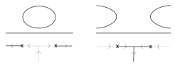
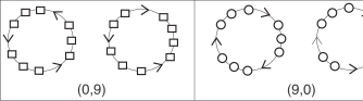
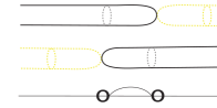
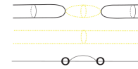
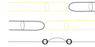
For the sake of simplicity, we first focus on fibrations which admit a real section. By a real section, we understand a section such that . Now, let be the real locus of the directed real elliptic Lefschetz fibration admitting a real section and having real critical values. We introduce a decoration on the base space as follows. First, we label the critical values of by “” or “” according to the parity of indices of the corresponding critical points. Namely, if the corresponding critical point is of index 1, we label the critical value by “”, otherwise by “”. (Note that has critical values as long as has real critical values.) We now consider a labeling on the set of regular intervals, , of . Existence of a real section assures that fibers of are never empty, so there are only two possible topological types for regular fibers: or . Over each regular interval the topology of the fibers of is fixed; moreover, it alternates as we pass through a critical value. We label regular intervals over which fibers have two components by doubling the interval, see Figure 1. Regular intervals over which the fibers of are a copy of remain unlabeled.
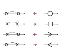
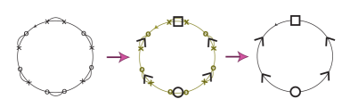
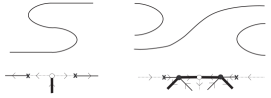
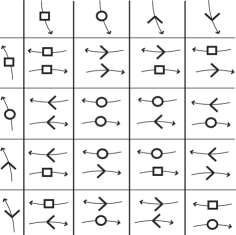
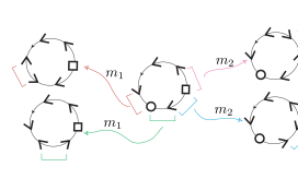
Oriented together with such a decoration, is called an oriented uncoated necklace diagram. Let us now consider “standard” pieces of the uncoated necklace diagrams out of which we can built all possible uncoated necklace diagrams. To avoid the matching problem of real structures, we deal with pieces of two critical values. Let us choose a regular value on . (For some later use we choose the point on an unlabeled regular interval.) With respect to this point and the orientation of , we have 4 instances for a pair of two critical values. In order to simplify the decoration, for each instance we introduce new notations as shown in Figure 2.
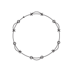
The oriented decorated using elements of the set is called an oriented necklace diagram (an example is shown in Figure 3). We call the elements of the set (necklace) stones and the pieces of the circle between the stones (necklace) chain. Two oriented necklace diagrams are considered identical if they contain the same types of stones going in the same cyclic order.
Remark 2.1.
It is obvious from the construction that oriented necklace diagrams are invariants of directed real elliptic Lefschetz fibrations.
When we consider non-directed real Lefschetz fibrations, we do not have a preferable orientation on the necklace diagram.
Non-directed fibrations, hence, determine a pair of oriented necklace diagrams related by a mirror symmetry in which ![]() -type and
-type and ![]() -type stones remain unchanged, while -type and -type stones interchanged.
-type stones remain unchanged, while -type and -type stones interchanged.
3. Monodromy representations of stones
As discussed in [5], monodromies of real Lefschetz fibrations around certain loops (namely, loops on which the real structure acts as a reflection) break up into a composition of two real structures. In particular, the monodromy around a single real singular fiber can be written as where denotes the positive Dehn twist along the vanishing cycle on a nearby marked (non-real) fiber identified with an abstract surface , and are the real structures pulled from the nearby right and respectively left real fibers (see [5, Theorem 2]). Using this decomposition, to each decoration around a critical value, we assign a certain matrix. These matrices are closely related to the monodromies of the fibrations.
Let us first recall that each real structure, , induces an isomorphism on that defines two rank 1 subgroups of . Moreover, if the real structure is separating, then . If is non-separating with one real component, then .
Remark 3.1.
By definition of real Lefschetz fibrations, around each critical point and critical value we have equivariant local (closed) charts , such that is equivariantly isomorphic to either of , where and with . In the case of (this is the model for the critical point of index 0, 2) there are two types of real regular fibers distinguished by their real parts. In both cases, one can choose invariant representatives for vanishing cycles and the action of the real structure on the invariant representative can be either the antipodal map or the identity. On the other hand, in the case of (this is the case of critical points of index 1) real structure acts on the invariant representative of the vanishing cycle as a reflection. Consequently, in the former situation ( which corresponds to the decoration “”) the class of the vanishing cycle gives an element in , while in the latter case (the case corresponding to the decoration “”) the class of the vanishing cycle gives an element of . (A detailed discussion about the local models can be found in of [6, Section 3] where the above claims are depicted in Figure 2.)
Lemma 3.2.
For each decoration around a critical value, we obtain the following matrices defined up to sign.
Proof: The explicit calculations will be made for , the other cases are similar.
Let be the critical value decorated by “”. We consider a sufficiently small -neighborhood of such that and . We mark a non-real point on and consider the shortest paths on from to the left and right real points of . By means of these paths, we pull the real structures on back to . Let us also fix an auxiliary identification with the fiber . Let (respectively ) be the real structures obtained by pulling back the real structure on (respectively ).
As discussed in Remark 3.1, the critical value of the type “” provides a generator of . Let denote the corresponding vanishing cycle and the homology class of . We have . We choose a generator for such that . As the decoration asserted, has one real component, so we want .
From the local monodromy decomposition, , we get ; therefore, and .
Obviously, the class , while .
We set and so that generates .
The matrix associated to the decoration is, then, which is the transition matrix from the base to the base .
Remark 3.3.
Intuitively, the monodromy assigned to a decoration around a critical value can be interpreted as the half of the monodromy around the real critical value, see Figure 4. We observe that where denotes the matrix of with respect to the base . Similarly, we have as well as and . Moreover, we have and where .

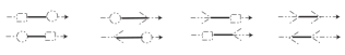
Therefore, to each necklace stone, we assign the following products (defined up to sign).
It is known that mapping class group, is isomorphic to the group . Let be identified with . We set and . Then, we consider two presentations of as follows.
Let us note one can switch from the first presentation to the second by setting and . Since , we have .
Remark 3.4.
Because we choose a point on an unlabeled interval, the matrices have coefficients in . If we marked a regular value on an labeled interval, the matrices we get would be elements of . (The reason why we prefer a point on an unlabeled interval is to get a nice relation between necklace stones and the real part (see Remark 4.5). ) The subgroup generated by is conjugate to . To be able work with , we consider the following lemma.
Lemma 3.5.
Let and .
Then, for each necklace stone we obtain the following factorization.
Proof:
The proof follows from the observation that
, while
The matrices are called monodromies of stones. The product of monodromies of necklace stones is called the monodromy of a necklace diagram.
Lemma 3.6.
Let be a directed totally real elliptic Lefschetz fibration admitting a real section. Then, the monodromy of the oriented necklace diagram associated with is the identity in .
Proof: Let be the ordered set of real critical values of . By means of underlying uncoated necklace diagram, we can write the monodromy of the necklace diagram as the product where is the matrix associated to the decoration around . Following Remark 3.3, we can write the monodromy along a curve surrounding all real critical values can be written as the product (see Figure 5)
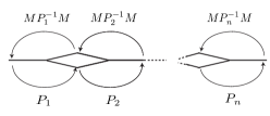
If there is no non-real critical value, the monodromy along the curve we consider is identical to the total monodromy of the fibration which is the identity.
Thus, we get . The equality assures that is the identity in .
Remark 3.7.
An important observation is that and
. Hence, if a necklace diagram has
the identity monodromy, then the necklace diagram obtained from the original by replacing
each ![]() -type stone with
-type stone with ![]() -type stone, and each
-type stone with -type stone and vice versa, has also the identity monodromy. Necklace diagrams obtained in this manner are called dual necklace diagrams.
-type stone, and each
-type stone with -type stone and vice versa, has also the identity monodromy. Necklace diagrams obtained in this manner are called dual necklace diagrams.
Remark 3.8.
Although for the moment, we focus on fibrations admitting a real section, it is worth mentioning the case of real structures with no real component. Indeed, real structures with no real component and those structures with two real components are are isotopic to each other as orientation reversing diffeomorphisms, although they are two non-isotopic real structures. As a result, they induce the same isomorphism on the homology group; hence, monodromy calculations remain the same if the real structure with two real components is replaced by a real structure with no real component.
4. The correspondence theorems and consequences
Theorem 4.1.
There exists a one-to-one correspondence between the set of oriented necklace diagrams with stones whose monodromy is the identity and the set of isomorphism classes of directed totally real elliptic Lefschetz fibrations , , that admit a real section.
Proof: From the discussions of the previous sections and by Lemma 3.6, we have an injection the set of fibrations to the set of diagrams. We want to show that this map is well-defined and surjective.
The crucial observation is that each necklace diagram with identity monodromy defines uniquely, up to cyclic order, a real Lefschetz chain of conjugacy classes of real codes. Let us recall that a real code is a pair consisting of a simple closed curve and a real structure on the fiber such that . As shown in [6], conjugacy classes of real codes are complete invariants of equivariant neighborhoods of real singular fibers of a real Lefschetz fibration. A real Lefschetz chain of conjugacy classes of real codes is a chain of codes such that is conjugate to .
To understand the relation between a necklace diagram and a real Lefschetz chains, it is enough to investigate the decorations of the underlying uncoated necklace diagram.
By definition, the decoration on regular intervals determine the conjugacy classes of real structures on the fibers over this interval.
By Remark 3.1, the decoration on the critical value determines the isotopy class of the vanishing cycle (invariant under the action of the real structure). The decoration around a critical value, hence, dictates the conjugacy class of a real code. An oriented necklace diagrams, hence, defines an ordered sequence of the conjugacy classes of real codes, so defines a real Lefschetz chain up to cyclic order. The result, therefore, follows from [6, Proposition 16].
Remark 4.2.
As mentioned in Remark 3.6 of [6], in the case when the regular fibers are tori, there are 6 conjugacy classes of real codes. Whereas, around each critical value we have 4 different decorations . These decorations are exactly 4 of the 6 possible real codes on . The other two cases appear in the case of non-existence of a real section that we discuss in the last section.
Corollary 4.3.
There exists a bijection between the set of symmetry classes of non-oriented necklace diagrams with stones whose monodromy is the identity, and the set of isomorphism classes of non-directed totally real , which admit a real section.
Each necklace diagram defines a decomposition of the identity in into a product of elements that are chosen from the set of monodromies of necklace stones. There is a simple algorithm to find all necklace diagrams associated with . Applying the algorithm, we obtain the complete list of necklace diagrams of . Later Andy Wand wrote a computer program for .
The following theorem concerns .
Theorem 4.4.
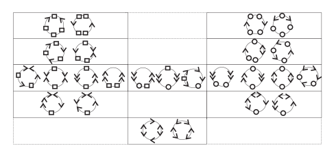
There exist precisely 25 isomorphism classes of non-directed totally real admitting a real section. These classes are characterized by the non-oriented necklace diagrams presented in Figure 6.
Proof:
By Theorem 4.3, it is enough to find the list of
symmetry classes of necklace diagrams of stones whose
monodromy is the identity. Each necklace diagram defines a decomposition of the identity in into a product of elements .
Let . To find all decompositions, we first consider all the words of length of letters such that the product is the identity.
We, then, quotient out the words which are equivalent to each other up to cyclic ordering. This way we obtain all oriented necklace diagrams which have the identity monodromy.
As a final step, we quotient out the symmetry classes. In terms of words composed of the letters , symmetry classes can be interpreted as follows: two words are considered to be equivalent if one is the reversed of the other with each is replaced by , and vice versa. For example, .
It is worth mentioning here that there are 8421 many necklace diagrams of 12 stones with the identity monodromy. Below, in Proposition 4.9, we give explicit list of necklace diagrams corresponding to certain classes. Later, we also explore some interesting examples.
Remark 4.5.
The topological invariants of can be read from the necklace diagram of .
Namely, we have and where denotes the Betti number of and
, denote the number of ![]() -type and respectively
-type and respectively ![]() -type stones of the necklace diagram associated with .
Consequently, we have the Euler characteristic , and the total Betti number .
-type stones of the necklace diagram associated with .
Consequently, we have the Euler characteristic , and the total Betti number .
Recall that in general we have (known as Smith inequality). It is known that ([2]), so we have .
Definition 4.6.
A real structure on is called maximal if . A necklace diagram maximal if .
We have the following immediate consequences.
Proposition 4.7.
Each necklace diagram whose monodromy is the identity contains at least two arrow type stones.
Corollary 4.8.
A totally real elliptic Lefschetz fibration admitting a real section contains at least two critical values of type
There are 4 maximal whose necklace diagrams that are depicted on the top line of Figure 6. For we have:
Proposition 4.9.
There are 10 isomorphism classes of maximal non-directed totally real admitting a real section.
Corresponding necklace diagrams are given Figure 7.
5. Applications of necklace diagrams
In this section, we study the algebraic realization of the totally real elliptic Lefschetz fibrations admitting a real section. The crucial observation is that any algebraic elliptic Lefschetz fibration admitting a real section can be seen as the double branched covering of a Hirzebruch surface of degree , branched at the exceptional section and a trigonal curve disjoint from the section. Orevkov [7] introduced a real version of Grothendieck’s dessins d‘enfants for the trigonal curves, which are disjoint from the exceptional section, on Hirzebruch surfaces. We apply his result by converting language of real dessin d’enfants to the language of necklace diagrams.
5.1. Trigonal curves on Hirzebruch surfaces
The Hirzebruch surface, , of degree is a complex surface equipped with a projection, , which defines a -bundle over with a unique exceptional section such that . In particular, and is blown up at one point.
Each Hirzebruch surface can be obtained from by a sequence of blow-ups followed by blow-downs at a certain set of points. If these points are chosen to be real, then the resulting Hirzebruch surface has a real structure inherited from the real structure on . This will be the real structure of our consideration. With respect to this real structure, the real part of is a torus if is even; otherwise it is a Klein bottle.
In this note, we only consider nonsingular curves, so by a trigonal curve on a Hirzebruch surface we understand a smooth algebraic curve such that the restriction of the bundle projection, , to is of degree 3. A trigonal curve on is called real if it is invariant under the real structure of .
5.2. Real dessins d’enfants of trigonal curves
We choose affine (complex) coordinates for such that the equation corresponds to fibers of and is the exceptional section . Then, with respect to such affine coordinates any (algebraic) trigonal curve can be given by a polynomial of the form where and are real one variable polynomials such that and .
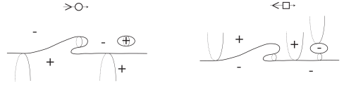
The discriminant of with respect to is . Let . The fraction is the -invariant of a trigonal curve . The -invariant defines a real rational function whose poles are the roots of , zeros are the roots of (taken with multiplicity 3), and the solutions of are the roots of (taken with the multiplicity 2).
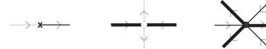
Let us color as in Figure 8. Then, the inverse image turns naturally into an oriented colored graph on . Since is real, the graph is symmetric with respect to the complex conjugation on . Around the vertices the graph looks as shown Figure 9. (Detailed discussion on -invariant of trigonal curves can be found in cf. [1], [7].)
The following theorem gives the conditions which are sufficient for the (real) algebraic realizability of a graph and the existence of respective polynomials .
Theorem 5.1.
[7]
Let be an embedded oriented graph where each of its edges is one of the three kinds: and some of its vertices are colored by the elements of the set , while others remains uncolored. Let satisfy the following conditions:
(1) The graph is symmetric with respect to an equator of , which is included
into ;
(2) The valency of each vertex is divisible by , and the incident edges are colored alternatively by incoming ![]() , and outgoing
, and outgoing ![]() ;
;
(3) The valency of each vertex is divisible by 4, and the incident edges are colored alternatively by incoming ![]() , and outgoing
, and outgoing ![]() ;
;
(4) The valency of each vertex is 2, and the incident edges are colored alternatively by incoming ![]() , and outgoing
, and outgoing ![]() ;
;
(5) The valency of each non-colored vertex is even, and the incident edges are of the same color;
(6) Each connected component of is homeomorphic to an open disc whose boundary is colored as a
covering of (colored and oriented as in Figure 8) and the orientations of the boundaries of neighboring discs are opposite.
Then, there exists a real rational function whose graph is .
(And thus, there exist a non-singular real algebraic trigonal curve associated to the invariant.)
Definition 5.2.
A graph on satisfying the conditions (1)-(6) of the above theorem is called a real dessin d’enfant.
Remark 5.3.
Let us accentuate the fact that there is no relation between the decorations “” of the critical values that we use to introduce the necklace diagrams and the coloring of the vertices of the real dessin d’enfants considered in this section.
5.3. Correspondence between real schemes and real dessins d’enfants
The real scheme of a trigonal curve imposes strong restrictions on the arrangement of the real roots of , and . For example, the zeros of correspond to the points where the trigonal curve is tangent to the fibers of . A typical correspondence for certain model pieces of the curve is shown in Figure 10. Because the graph is symmetric with respect to the equator, we consider the part of the graph lying on one of the half discs.
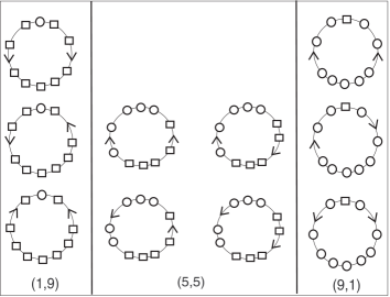
As we mention in the previous section, necklace diagrams encode the topology of the real part (except orientability) of which admit a real section. Indeed, the real part of totally real , admitting a real section, consists of spherical components (the number of which is ) and a higher genus component which is an orientable surface of genus if is even; a non-orientable surface with cross-caps, otherwise.
Definition 5.4.
A segment of a necklace diagram is called essential if the corresponding graph fragment contains at least one “” type vertex and at least two “” type vertices. (Essential segments are listed in Figure 11.)
5.4. Applications
Proposition 5.5.
If a real elliptic Lefschetz fibration, , admitting a real section is algebraic then the corresponding necklace diagram has the following properties:
-
•
there are not more than essential segments,
-
•
the sum of the number of essential segments and the number of arrow type stones cannot be greater then .
Proof:
For a trigonal curve on defined by , and .
Thus, the real dessin d’enfant can have at most vertices colored by “” and at most vertices colored by “”.
The result follows from the observation that each essential interval corresponds to a graph fragment which contains
at least two “” type vertices and at least one “” type vertex, while
each arrow type stone corresponds to a fragment having at least one “” type vertex.
Corollary 5.6.
The totally real elliptic Lefschetz fibrations corresponding to the necklace diagrams depicted in Figure 12 are not realized algebraically.

Proof:
It is easy to see that the diagram having only arrow type stones violates the second condition, while all the others violate the first condition stated in Proposition 5.5.
Lemma 5.7.
If a totally real elliptic Lefschetz fibration admitting a real section is algebraic then the totally real elliptic Lefschetz fibration whose necklace diagram is dual to the necklace diagram of the former is also algebraic.
Proof: The crucial observation is that although the real parts of fibrations associated with dual necklace diagrams are topologically different, trigonal curves appearing as the branching set of coverings are the same. Duality of necklace diagrams corresponds, indeed, to the two different liftings of the real structure of to , see Figure 13.
Theorem 5.8.
All totally real admitting a real section are algebraic except those fibrations whose necklace diagram is one of the diagrams listed in Figure 12.
Proof:
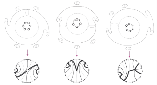
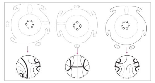
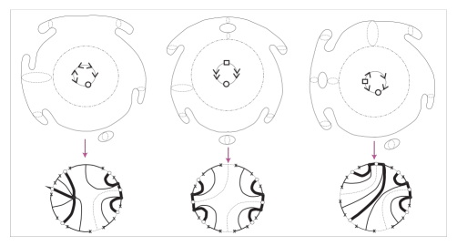
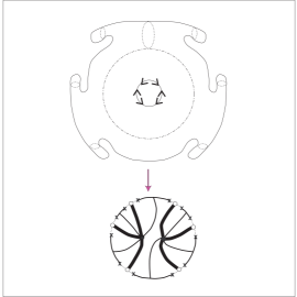
By Theorem 5.1 it is enough to construct real dessins d’enfants corresponding to necklace diagrams which are
not prohibited by Proposition 5.5.
Following Lemma 5.7, we only need to consider necklace diagrams with .
Figures 14-17 show the required real dessins d’enfants.
Real dessins d’enfants of real algebraic with real sections. (Around necklace diagrams, the real part is depicted. The dotted inner circle stands for the lift of the exceptional section. Because of the symmetry, we only draw a half of the graph.)
6. Necklace calculus and further applications
In this section, we consider certain operations on the set of necklace diagrams. These operations allow us to construct new necklace diagrams from the given ones.
6.1. Necklace sums
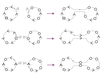
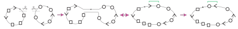
A necklace sum is basically the connected sum of the underlying oriented circle and it refers to the fiber sum of the corresponding real Lefschetz fibrations. We consider two types of necklace sums which we call mild sum and harsh sum. To perform a mild sum, we cut each necklace diagram at a point on the chain then reglue the diagrams crosswise respecting the orientation. The harsh sum, on the other hand, is obtained by cutting necklace diagrams at a stone and regluing them according to the table shown in Figure 18. It follows from their definition that both the mild sum and the harsh sum do not change the monodromy of the diagram. Evidently, the Euler characteristic is additive with respect to the mild sum; however, it is not always additive with respect to the harsh sum.
Let us note also that we can also consider necklace sum of non-oriented necklace diagram by fixing auxiliary orientations on diagrams.
Examples of mild and harsh sums are given in Figure 19.
Remark 6.1.
There are two types of necklace chain segments (essential, non-essential) distinguished by the associated graph fragments.
It is not hard to see that the mild sum preserves algebraicity if the points where the sum is taken are chosen on the same type of chain segments and if the segments after the sum remain of the same type; or if they are chosen on different types of chain segments. (In other words, algebraicity is preserved if we make a mild sum at two essential (respectively non-essential) intervals, in a way that after gluing we obtain again two essential (respectively non-essential) intervals; or if we make sum at an essential and a non-essential intervals.) As for the harsh sum, we note that it preserves algebraicity if the number of neither ![]() -type nor -type stone decreases after the sum.
-type nor -type stone decreases after the sum.
Proposition 6.2.
For each , maximal necklace diagrams exist and each totally real elliptic represented by a maximal necklace diagram is algebraic.
Proof: It is easy to see that the harsh sum of two maximal necklace diagrams where the sum is performed at arrow type stones of the opposite directions is maximal. Moreover, by the remark above harsh sum performed at two arrow type stones of opposite directions preserves algebraicity. Note also that as Theorem 5.8 asserted all maximal necklace diagrams of 6 stones are algebraic.
To finish the proof, we show that all maximal necklace diagrams of stones are obtained as harsh sums of maximal necklace diagrams of 6 stones.
We will prove the claim by induction on .
The first step is to check the claim for . As we have the explicit list of maximal diagrams of 12 stones, we see immediately that any maximal necklace diagram of 12 stones can be obtained as the harsh sum of maximal necklace diagrams of 6 stones.
Now, let us assume that for the claim is true.
To prove the claim for , note that the monodromies of ![]() -type stones and
-type stones and ![]() -type stones do not have any cancelation.
The fact that there is no cancellation between
-type stones do not have any cancelation.
The fact that there is no cancellation between ![]() -type stones and
-type stones and ![]() -type stones and that the monodromy of the necklace diagram is the identity
impose certain conditions on the possible arrangements of stones around an arrow type stone on a maximal necklace diagram.
By checking the possibilities of the neighborhood of an arrow type stone, we see that required cancelations appear only in the cases where the arrangements come from the maximal necklace diagrams of 6 stones, so the claim follows from the inductive step.
-type stones and that the monodromy of the necklace diagram is the identity
impose certain conditions on the possible arrangements of stones around an arrow type stone on a maximal necklace diagram.
By checking the possibilities of the neighborhood of an arrow type stone, we see that required cancelations appear only in the cases where the arrangements come from the maximal necklace diagrams of 6 stones, so the claim follows from the inductive step.
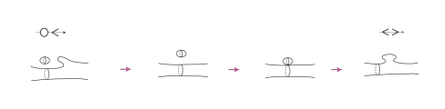
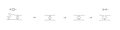
6.2. Flip-flops and metamorphoses
Let denote the set of (oriented) necklace diagrams with stones and with the identity monodromy, and let be the subset consisting of diagrams with . We define two kinds of operations on : flip-flop and metamorphosis. The flip-flop preserves and it coincides with canceling and creating handles on the real part . On the other hand, the metamorphosis decreases or by one and it appertains to a nodal deformation of .
Flip-flop is the operation which swaps the segments shown below. Because the segments have the same monodromy, the total monodromy does not change. Examples of flip-flop are shown in Figure 20.
As and remain unchanged after a flip-flop, the Euler characteristic and the total Betti number of the corresponding do not change. Thus, topological type of is not affected by the flip-flop. In Figure 21, we interpret the effect of a flip-flop on .
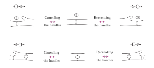
We consider two types of metamorphoses, , of necklace diagrams. They modify the stones of the above segments as below. Examples of metamorphoses are depicted in Figure 22.
Since or are modified by metamorphoses, the topological type of the corresponding changes. Recall that for fibrations which admit a real section each ![]() -type stone corresponds to a spherical component while each
-type stone corresponds to a spherical component while each ![]() -type stone drives a handle. Indeed, a sphere component or a genus disappears after a metamorphosis (or appears after a inverse metamorphosis). In Figure 23, we depict the effects of metamorphoses on .
-type stone drives a handle. Indeed, a sphere component or a genus disappears after a metamorphosis (or appears after a inverse metamorphosis). In Figure 23, we depict the effects of metamorphoses on .
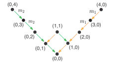
6.3. Applications
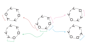
Below, in Figure 24 and Figure 25, we present two graphs (for and , respectively) whose vertices correspond to necklace diagrams with fixed , edges to necklace metamorphoses . As we mention before the real part of totally real , admitting a real section, consists of spherical components (the number of which is ) and a higher genus component which is an orientable surface of genus if is even; a non-orientable surface with cross-caps, otherwise. Each pair and the parity of , thus, defines the topological type of .

Examining the list of necklace diagrams of 6 stones we obtain the following:
Proposition 6.3.
All 6-stone necklace diagrams listed in Figure 6 can be obtained from the maximal ones by a sequences of metamorphoses, inverse metamorphoses or flip-flops.
Moreover, the list of necklace diagrams which are obtained from maximal diagrams only by a sequence of metamorphoses and eventually an inverse metamorphosis, coincide with the list of diagrams of algebraic fibrations.
Proposition 6.4.
There exist 12-stone necklace diagrams (with the identity monodromy) that can not be obtained from the maximal necklace diagrams by necklace operations.
Proof: By duality it is enough to consider the case of . Examples, shown in Figure 26, are found by investigating the list of 12-stone necklace diagrams basically with . Let us also note that the fibrations associated with the diagrams shown in Figure 26 are algebraic.
As a corollary of the above proposition we claim that all totally real algebraic admitting a real section can be obtained from the maximal ones by a sequences of nodal deformations, while there are totally real algebraic which cannot be obtained in this way.
Proposition 6.5.
There exist 12-stone necklace diagrams (with the identity monodromy) which are not a necklace sum of two 6-stone necklace diagrams listed in 6.
Proof: In Figure 27, we construct a non-decompasable example applying a mild sum followed by a flip-flop. Let us also note that such examples can be produced the same way for any .
By analyzing possible divisions of the pair , we see that the necklace diagram shown in
Figure 27 cannot be divided into two 6-stone necklace
diagrams with the identity.
Corollary 6.6.
There exist totally real which cannot be written as a fiber sum of two totally real .
7. Totally real elliptic Lefschetz fibrations without a real section and refined necklace diagrams
In this section, we explore the case of totally real elliptic Lefschetz fibrations which do not admit a real section and introduce refined necklace diagrams associated with them.
A refinement of a necklace diagram is obtained by replacing each ![]() -type stone with one of the following refined stones, .
If the refined necklace diagram is identical to the underlying necklace diagram then the corresponding real Lefschetz fibration admits a real section.
Examples of refinements of a necklace diagram are shown in Figure 28.
-type stone with one of the following refined stones, .
If the refined necklace diagram is identical to the underlying necklace diagram then the corresponding real Lefschetz fibration admits a real section.
Examples of refinements of a necklace diagram are shown in Figure 28.
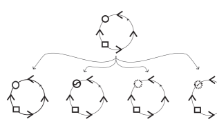
From Remark 3.1, it is clear that if a real structure on a fiber of has no real component, then the nearby critical values can only be of type “”. In other words, existence or lack of a real section influences only ![]() -type necklace stones.
-type necklace stones.
Both of the refined stones of type correspond to the case where the real structure on the real fibers over the interval between the two critical values has 2 real components.
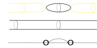
Already the real part of distinguishes the cases of ![]() and
and ![]() , see Figure 29. As notation suggested
, see Figure 29. As notation suggested ![]() has to do with the case where there is a real section, and hence, only
has to do with the case where there is a real section, and hence, only ![]() -type refined stones refer to a spherical component of .
-type refined stones refer to a spherical component of .
Recall that if the condition that the fibration admits a real section is discarded, then the fibers of may also be empty (which happens when the real structure on the real fibers of has no real component). We introduce the refined stones ![]() and
and ![]() which correspond to the case where the real structure on the real fibers of has no real component.
As depicted in Figure 30, the real part of does not distinguish the two situations associated with .
The difference between
which correspond to the case where the real structure on the real fibers of has no real component.
As depicted in Figure 30, the real part of does not distinguish the two situations associated with .
The difference between ![]() and
and ![]() (as well as between
(as well as between ![]() and
and ![]() ) can indeed be conceived by comparing the equivariant isotopy classes of
the two vanishing cycles corresponding to the two critical values of the necklace stone. In the case of
) can indeed be conceived by comparing the equivariant isotopy classes of
the two vanishing cycles corresponding to the two critical values of the necklace stone. In the case of ![]() (respectively
(respectively ![]() ) the equivariant isotopy classes of vanishing cycles are the same, while in the case of
) the equivariant isotopy classes of vanishing cycles are the same, while in the case of ![]() (respectively,
(respectively, ![]() )
the two vanishing cycles are of different equivariant classes. (A more detailed discussion can be found in [6, Section 8].)
)
the two vanishing cycles are of different equivariant classes. (A more detailed discussion can be found in [6, Section 8].)
As mentioned in Remark 3.8, there is no difference between real structures with 2 real components and real structures with no component on the homological level. As a consequence, the calculation of the monodromy does not affected by the refinement. Thus, we have the following theorem.
Theorem 7.1.
There is a one-to-one correspondence between the set of oriented refined necklace diagrams with stones whose monodromy is the identity and the set of isomorphism classes of directed totally real , .
Proof: The proof is analogous to the proof of Theorem 4.1.
It is obvious from its construction that the refinements of necklace diagram is exactly the decoration of the real Lefschetz chains, see Figrure 10 of [6]. Thus, we relate refined necklace diagrams with the decorated real Lefschetz fibrations, complete invariants of totally real elliptic Lefschetz fibrations, presented in [6, Section 8].
The result, thus, follows from Theorem 8.1 and Proposition 8.2 of [6].
Corollary 7.2.
There is a one-to-one correspondence between the set of symmetry classes non-oriented refined necklace diagrams with stones whose monodromy is the
identity and the set of isomorphism classes of totally real , .
The number of possible refinements of necklace diagrams with fixed listed Figure 6 is given below.
-
•
there are 12 refined necklace diagrams,
-
•
there are 8 refined necklace diagrams,
-
•
there are 46 refined necklace diagrams,
-
•
there are 84 refined necklace diagrams,
-
•
there are 251 refined necklace diagrams.
References
- [1] Degtrayev, A.; Itenberg I.; Kharlamov V. On Deformation types of real elliptic surfaces. American Journal of Mathematics, Volume 130, Number 6, 2008, 1561-1627.
- [2] Gompf, R.E., A.I. Stipsicz 4-manifols and Kirby calculus. Amer. Math. Soc. Grad. Stud. in Math. 20 Rhode Island, (1999).
- [3] Kulikov, S.; Kharlamov, V. On real structures on rigid surfaces. (Russian) Izv. Ross. Akad. Nauk Ser. Mat. 66 (2002), no. 1, 133–152; translation in Izv. Math. 66 (2002), no. 1, 133 150.
- [4] Moishezon, B. Complex surfaces and connected sums of complex projective planes. Lecture notes in Math. 603 Springer Verlag(1977)
- [5] Salepci, N. Real classes in the mapping class group of , Topology and its Applications, Volume 157, Issue 16, 2010, 2480-2590.
- [6] Salepci, N. Invariants of totally real Lefschetz fibrations, submitted preprint, arXiv:1101.1380v1.
- [7] Orevkov, S.Yu. Riemann existence theorem and construction of real algebraic curves. Ann. Fac. Sci. Toulouse Math. (6)12, 2003, no. 4, 517-531.