Kosterlitz-Thouless transition of magnetic dipoles on the two-dimensional plane

Abstract

The universality class of a phase transition is often determined by factors like dimensionality and inherent symmetry. We study the magnetic dipole system in which the ground-state symmetry and the underlying lattice structure are coupled to each other in an intricate way. A two-dimensional (2D) square-lattice system of magnetic dipoles undergoes an order-disorder phase transition belonging to the 2D Ising universality class. According to Prakash and Henley [Phys. Rev. B 42, 6572 (1990)], this can be related to the fourfold-symmetric ground states which suggests a similarity to the four-state clock model. Provided that this type of symmetry connection holds true, the magnetic dipoles on a honeycomb lattice, which possess sixfold-symmetric ground states, should exhibit a Kosterlitz-Thouless transition in accordance with the six-state clock model. This is verified through numerical simulations in the present investigation. However, it is pointed out that this symmetry argument does not always apply, which suggests that factors other than symmetry can be decisive for the universality class of the magnetic dipole system.

Understanding the physics in thin films is of practical importance since thin-film construction is used in manufacturing a variety of electronic and optical devices. One may note that magnetic thin films, in particular, play a key role in massive data storage applications and that magnetic interactions in such films will become more prominent as magnetic moments are more densely integrated on such devices. A typical behavior of the magnetic property in thin films is switching between perpendicular and in-plane magnetization as the temperature $T$ varies, which was first reported for Fe films. pappas On the other hand, for rare-earth compounds such as ErBa₂Cu₃O_6+x, the ordering of magnetic spins at $T<1.0$K is essentially two-dimensional (2D). lynn For these materials, the exchange interaction is known to be relatively weak, mac and the rare-earth ionic moments have been described as Ising or $XY$ spins depending on anisotropy. simizu These compounds have also attracted attention as a suitable candidate to reveal the relation between superconductivity and magnetism. A model of a magnetic thin film is therefore a 2D lattice of magnets governed by the dipole interaction and confined to rotate on the plane of the lattice. Although it is straightforward to write down the corresponding Hamiltonian, understanding its physics is more cumbersome, for two reasons: the long-range character of the dipole interaction and its anisotropy. For a lattice of $N$ planar magnets with the dipole interaction, the Hamiltonian is given as follows:

$$H=J\sum_{i\neq j}\left[(\boldsymbol{s}_{i}\cdot\boldsymbol{s}_{j})r_{ij}^{2}-3(\boldsymbol{s}_{i}\cdot\boldsymbol{r}_{ij})(\boldsymbol{s}_{j}\cdot\boldsymbol{r}_{ij})\right]/r_{ij}^{5},$$ (1)

where $J(>0)$ is a coupling constant and the summation runs over all the distinct spin pairs $\boldsymbol{s}_{i}$ and $\boldsymbol{s}_{j}$, residing at $\boldsymbol{r}_{i}$ and $\boldsymbol{r}_{j}$, respectively. The distance between members of a spin pair is denoted as $r_{ij}=\left|\boldsymbol{r}_{i}-\boldsymbol{r}_{j}\right|$. Since we employ the periodic-boundary condition, the displacement $\boldsymbol{r}_{ij}$ between $\boldsymbol{r}_{i}$ and $\boldsymbol{r}_{j}$ is chosen as the one with the minimal distance among every possible pair of their periodic images. If more than two periodic images of a spin have the same minimal distance from another spin, we neglect the interaction between members of this spin pair to remove the ambiguity. As is clearly seen in Eq. (1), the interaction energy between $\boldsymbol{s}_{i}$ and $\boldsymbol{s}_{j}$ decays as $r_{ij}^{-3}$ and it does not depend solely on their angular difference but also on their relative position, $\boldsymbol{r}_{ij}$. In terms of numerical analysis, the long-range character imposes an $O(N^{2})$ complexity within the simple Metropolis algorithm and the anisotropy puts an obstacle to developing an effective cluster algorithm. These problems have left the properties of the phase transition in this system largely inconclusive. On the one hand, this dipole lattice is related to the ice model, bark which undergoes a phase transition keeping its structural arrangement disordered. bram The lack of a long-range order has been reported in the neutron-scattering experiments for some rare-earth compounds clinton and also in artificial spin ice. wang On the other hand, such disorder-preserving behavior apparently disagrees with theoretical and numerical predictions that the long-range order will be established in the 2D dipole lattice at low $T$. debell1 ; debell2 ; car Even if we accept the existence of an order-disorder transition at a critical temperature $T_{c}$ in the dipole system, numerical studies produce conflicting results: For the case of a square lattice, there has been reported a value of the critical exponent $\beta=0.19(4)$ for the staggered magnetization as well as $\gamma=1.37(7)$ for the staggered susceptibility with the correlation-length exponent $\nu=1$, car ; ras where the numbers in the parentheses are numerical errors in the last digits. The staggered magnetization vector is defined as $\boldsymbol{m}=N^{-1}\sum_{i}\boldsymbol{\sigma}_{i}$, where we specify the components of the vectors as $\boldsymbol{r}_{i}=(x_{i},y_{i})$ and $\boldsymbol{s}_{i}=(\cos\theta_{i},\sin\theta_{i})$, respectively, and define gauge-transformed spins as debell1

$$\boldsymbol{\sigma}_{i}\equiv\left[(-1)^{y_{i}}\cos\theta_{i},(-1)^{x_{i}}\sin\theta_{i}\right].$$ (2)

We take the magnitude $m=\left|\boldsymbol{m}\right|$ as a scalar magnetic-order parameter of this system. Using the same observable, a recent study reported $\beta/\nu=0.13(2)$ and $\nu=1.05(5)$ with the Metropolis algorithm. fer This result indicates the 2D Ising universality class within errors, which is partially supported by another study on the Heisenberg dipole system. tomita However, none of these match a renormalization-group calculation maier yielding an exponentially diverging correlation length $\xi$ with $\log\xi\sim 1/\sqrt{T-T_{c}}$ and magnetization $\sim\xi^{-1/2}$. To our knowledge, no theoretical explanation of the observed results has been satisfactorily provided.

In this brief report, we begin with the critical behavior of magnetic dipoles on the square lattice. The finite-size scaling result from $L\times L$ square lattices supports an order-disorder transition with the 2D Ising universality class, confirming the recent observation. fer We then ask if this is related to the fact that the system possesses fourfold-symmetric ground states. debell1 To test this further, we use the fact that the magnetic dipoles may have sixfold-symmetric ground states if put on the honeycomb lattice. pra This has been well established for the nearest-neighbor dipole interaction, pra and we have numerically checked its validity for the long-range-interaction case as well. We find that the honeycomb-lattice lattice case exhibits a Kosterlitz-Thouless (KT) transition as implied by the analogy to the six-state clock model. six ; nonkt

Our simulation strategy is as follows: we use the parallel tempering (PT) method that was devised to equilibrate glassy spin systems with very long relaxation times. exchange ; mc Consider simulating two samples of a spin system in parallel at different inverse temperatures, $\beta_{1}$ and $\beta_{2}$, respectively. If $\beta_{1}<\beta_{2}$, the sample at $\beta_{1}$ will explore a larger region in the phase space than will the sample at $\beta_{2}$. If the exploration happens to find a state with sufficiently low energy, we exchange $\beta_{1}$ and $\beta_{2}$ of the two samples so that the low-energy state can be pursued more deeply while the other sample begins a new exploration. Specifically, if energies of the two samples are denoted $E_{1}$ and $E_{2}$, respectively, the exchanging probability is given as $P_{\rm ex}=\min\left\{1,\exp\left[-(\beta_{2}-\beta_{1})(E_{1}-E_{2})\right]\right\}$ to satisfy the detailed balance. One may easily extend this scheme to more than two samples, ranging over a broad temperature region, and run the samples simultaneously on parallel computing devices. We simulate each sample by the Metropolis algorithm, which means that the overall complexity is still $O(N^{2})$. Only its proportionality coefficient will be reduced by application of the PT method, but it is nevertheless a significant gain in practice especially when $N$ is not too large. For $L=32$ in Fig. 1(a), for example, it usually takes $10^{4}\sim 10^{5}$ Monte Carlo steps for a simple Metropolis algorithm to equilibrate the system around $T_{c}$ from a random configuration, while it is enough to make a couple of exchange moves with running $O(10^{3})$ steps in between. We determine the difference in inverse temperature by observing overlaps of energy histograms. In the same example ($L=32$), we have simultaneously simulated $31$ inverse temperatures over $[1.03,1.63]$, each of which runs on an Intel Xeon quad-core L5420 CPU (2.5GHz). The CPU time spent for this size is about $6\times 10^{2}$ h per temperature, meaning that the total CPU time to obtain the result for $L=32$ roughly amounts to $2\times 10^{4}$ h.

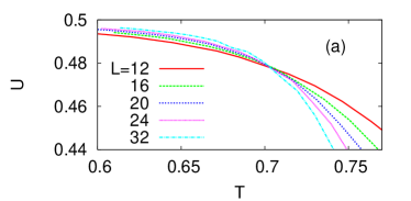
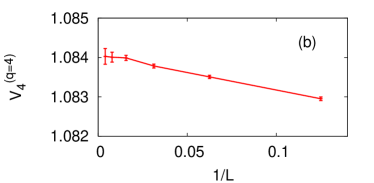
Figure 1: (Color online) (a) Binder’s cumulant of magnetic dipoles on $L\times L$ square lattices. (b) Cumulant ratio $V_{4}^{q=4}=\left<m^{4}\right>/\left<m^{2}\right>^{2}$ obtained for the 2D square-lattice four-state clock model at the critical temperature $T_{c}^{q=4}=1/\log(1+\sqrt{2})$.

Figure 1(a) shows Binder’s cumulant $U\equiv 1-\frac{1}{2}\left<m^{4}\right>/\left<m^{2}\right>^{2}$ from the staggered magnetization, where $\left<\cdots\right>$ means thermal average. Note that this cumulant is scaled to approach zero at high $T$ and $1/2$ at low $T$ since $\left<m^{4}\right>=2\left<m^{2}\right>^{2}$ when the magnetization vector $\boldsymbol{m}$ has a 2D Gaussian distribution centered at the origin. From Fig. 1(a), the transition temperature is estimated as $T_{c}=0.70(2)$ in units of $J/k_{B}$, where $k_{B}$ is the Boltzmann constant. Since this is not an extremely precise estimation, it is hard to get critical exponents to a good precision. Instead, we may check consistency by assuming the 2D Ising universality class.

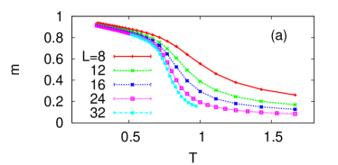
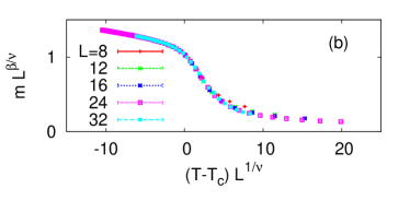
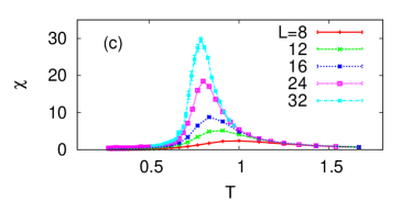
Figure 2: (Color online) Results on square lattices. (a) Staggered magnetization and its scaling collapse (b) according to the 2D Ising universality class. (c) Staggered susceptibility and its scaling collapse (d) in the same way. The 2D Ising critical exponents $\beta=1/8$, $\nu=1$, and $\gamma=7/4$ are used; and the critical temperature is estimated to be $T_{c}=0.71(1)$ and $0.72(1)$ for (b) and (d), respectively.

Let us plot the staggered magnetization and try a scaling collapse by the 2D Ising universality class, i.e., $\beta=1/8$ and $\nu=1$ [Figs. 2(a) and 2(b)]. The best collapse is observed at $T_{c}=0.71(1)$, which is in good agreement with the value of $T_{c}$ estimated above via Binder’s cumulant. Another important observable is the staggered susceptibility $\chi=NT^{-1}\left[\left<m^{2}\right>-\left<m\right>^{2}\right]$ plotted in Fig. 2(c). Again the 2D Ising universality class with the corresponding critical exponent $\gamma=7/4$ is clearly consistent with the data provided that $T_{c}=0.72(1)$ [Fig. 2(d)]. One also notes that the susceptibility data imply a single transition point where the critical fluctuation diverges in the thermodynamic limit, and that the susceptibility remains finite below this divergence. This rules out the possibility of a KT transition. The consistent descriptions strongly suggest that the critical behavior indeed belongs to the 2D Ising universality class.

It is obviously nontrivial that a continuous-spin system, complicated by the long-range character and anisotropy, nevertheless displays an Ising transition. The most plausible explanation is that the ground states of the dipole system on the square lattice possess a fourfold symmetry, debell1 since the same is true for the four-state clock model, which exhibits the 2D Ising criticality. suzuki The value of the cumulant indeed tells us more than this simple symmetry argument: Figure 1(a) shows that $V_{4}\equiv\left<m^{4}\right>/\left<m^{2}\right>^{2}=2(1-U)\approx 1.04(1)$. For the 2D Ising model, on the other hand, the value of this quantity is given as $V_{4}^{\rm Ising}=1+\epsilon$, where $\epsilon=0.167923(5)$. salas Since the four-state clock model is equivalent to two independent Ising systems $A$ and $B$ with the temperature rescaled, suzuki we can denote it as $A\otimes B$ and consider its magnetic-order parameter $m=\sqrt{(m_{A}^{2}+m_{B}^{2})/2}$ where $m_{A}$ and $m_{B}$ correspond to magnetizations of the independent Ising systems. This leads to the cumulant value of the four-state clock model as follows:

$$V_{4}^{(q=4)} = \frac{\left<(m_{A}^{2}+m_{B}^{2})^{2}\right>}{\left<m_{A}^{2}+m_{B}^{2}\right>^{2}}=\frac{\left<m_{A}^{4}\right>+2\left<m_{A}^{2}\right>\left<m_{B}^{2}\right>+\left<m_{B}^{4}\right>}{\left<m_{A}^{2}\right>^{2}+2\left<m_{A}^{2}\right>\left<m_{B}^{2}\right>+\left<m_{B}^{2}\right>^{2}}$$

$$= \frac{2+2V_{4}^{\rm(Ising)}}{4}=1+\frac{\epsilon}{2},$$

which agrees well with our Monte Carlo calculation $V_{4}^{q=4}=1.0840(2)$ at $T_{c}^{q=4}=1/\log(1+\sqrt{2})$ [Fig. 1(b)]. By the same analogy, the cumulant value for the magnetic dipoles suggests that $V_{4}=1+\epsilon/4\approx 1.042$, which could be observed in a combination of four independent Ising systems denoted as $A,B,C$, and $D$, respectively, or two independent four-state clock models $A\otimes B$ and $C\otimes D$, where the total magnetization is equivalent to $m=\sqrt{(m_{A}^{2}+m_{B}^{2}+m_{C}^{2}+m_{D}^{2})/4}$.

In order to test the symmetry argument further, we investigate the honeycomb lattice, since the nearest-neighbor dipole interaction in this case leads to sixfold ground states. pra In addition, since it is known that the $q$-state clock model with the cosine interaction undergoes a KT transition when $q\geq 6$, six ; nonkt the symmetry argument suggests that the transition for a honeycomb lattice should be of a KT type.

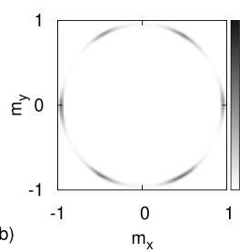
Figure 3: (a) Honeycomb lattice of size $L=6$ with the periodic-boundary condition. Coordinates are presented as $(u,w)$ for the gauge transformation in Table 1. (b) Distribution of staggered magnetization $\boldsymbol{m}=(m_{x},m_{y})$, showing the sixfold symmetry, taken at $T=0.1$ with $L=12$.

The honeycomb lattice that we use in this work is shown in Fig. 3(a) where the system size is $N=2L^{2}$ for a given length scale $L$. We choose $L$ as multiples of $6$ by taking the ground-state configurations pra into consideration. An appropriate gauge transformation of the spin angle $\theta$ at site $(u,w)$ in the same spirit of Eq. (2) is tabulated in Table 1. The staggered magnetization is defined as $\boldsymbol{m}=N^{-1}\sum(\cos\theta^{\prime},\sin\theta^{\prime})$ with magnitude $m\equiv|\boldsymbol{m}|$. As in the square-lattice case, each chosen spin interacts with a set of other spins that have well-defined minimal distances to the chosen spin. We furthermore require this interacting set to have the inherent symmetry of the honeycomb lattice; i.e., the interacting set should be left invariant under the rotation by $\pm 2\pi/3$ around the chosen spin so that the six ground states are equally probable in the system [Fig. 3(b)]. The numerical results are again obtained by the PT method and plotted in Figs. 4(a)-4(d), where Binder’s cumulant $U$ and the staggered susceptibility $\chi$ are given in the same way as above. In order to examine the low-$T$ phase, we have the inverse temperature range over $O(1)$ to $O(10)$ while keeping the overlaps in the energy histograms. For $L=24$, for example, we ran $127$ inverse temperatures over $[1.5,10.3]$ in parallel, spending about $10^{2}$ CPU hours per each. Around $T\approx 0.5$, one finds a size merging of $U$, together with a divergence in $\chi$, which are characteristic signatures of the KT transition. These observations imply the existence of a quasicritical phase below $T\approx 0.5$ where the correlation length diverges. The KT picture also predicts a scaling collapse of $\chi$ vs $U$, such that $\chi\sim L^{2-\eta}f(U)$ where $f$ is a certain scaling function and $\eta=1/4$. gqclock This method provides a piece of information about the universality class even without precise knowledge of the transition temperature. In spite of the small system sizes, the KT scaling exponent $\eta=1/4$ nevertheless gives a scaling collapse consistent with a KT transition as shown in the inset of Fig. 4(c). We also note an additional tiny yet systematic size dependence of $U$ below $T=0.2$ shown in the inset of Fig. 4(b), which possibly indicates that the staggered magnetization freezes into the sixfold symmetry [compare Fig. 3(b)]. Unlike in the six-state clock model, however, this freezing is not accompanied by any peak in specific heat [Fig. 4(d)], which implies that the quasicritical phase is not isotropic either but should reflect the sixfold symmetry at least in part. It is currently under investigation whether the $U(1)$ symmetry in the disordered phase gets broken exactly at the same temperature where the KT transition occurs.

Table 1: Gauge transformation for the honeycomb lattice, where $(u,w)$ represents the coordinates as shown in Fig. 3(a).

$u\mod 4$	$w\mod 3$	$\theta^{\prime}$	$u\mod 4$	$w\mod 3$	$\theta^{\prime}$	$u\mod 4$	$w\mod 3$	$\theta^{\prime}$
0	0	$\theta$	0	1	$\theta+2\pi/3$	0	2	$\theta-2\pi/3$
1	0	$-\theta$	1	1	$-\theta+2\pi/3$	1	2	$-\theta-2\pi/3$
2	0	$\theta-2\pi/3$	2	1	$\theta$	2	2	$\theta+2\pi/3$
3	0	$-\theta-2\pi/3$	3	1	$-\theta$	3	2	$-\theta+2\pi/3$

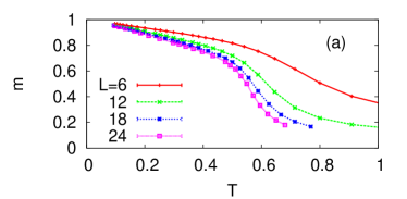
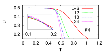
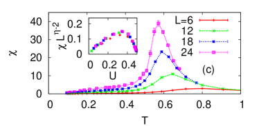
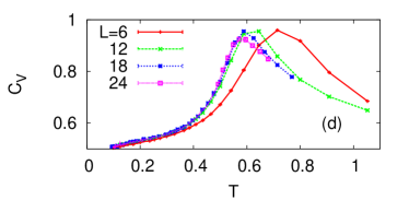
Figure 4: (Color online) Results on honeycomb lattices. (a) Magnitude of the staggered magnetization and (b) Binder’s cumulant, with a closer view of the low-$T$ part (inset). (c) Staggered susceptibility $\chi$ and the scaling collapse of $\chi\sim L^{2-\eta}f(U)$ with $\eta=1/4$. (d) Specific heat does not show any clear double-peak structure.

In summary, we have confirmed that the $XY$-type magnetic dipoles on the square lattice exhibit the 2D Ising criticality and that this can be related to a symmetry similarity in the four-state clock model. This symmetry connection is further supported by the study of the honeycomb lattice, where the ground states have sixfold symmetry; and the system behaves similarly to the six-state clock model exhibiting a KT transition. However, the symmetry argument is not always the decisive factor: the transition is KT-like for the square lattice with nearest-neighbor interaction in spite of the fact that the symmetry remains the same. romano One may also note that the long-range order at low $T$ is also absent in experiments with squarelike structures. clinton However, the factors that supersede the symmetry argument in deciding the critical universality class remain to be elucidated.

- (1) D. P. Pappas, K.-P. Kämper, and H. Hopster, Phys. Rev. Lett. 64, 3179 (1990).
- (2) J. W. Lynn, W.-H. Li, Q. Li, H. C. Ku, H. D. Yang, and R. N. Shelton, Phys. Rev. B 36, 2374 (1987).
- (3) A. B. MacIsaac, J. P. Whitehead, K. De’Bell, and K. S. Narayanan, Phys. Rev. B 46, 6387 (1992).
- (4) S. Simizu, G. H. Bellesis, J. Lukin, S. A. Friedberg, H. S. Lessure, S. M. Fine, and M. Greenblatt, Phys. Rev. B 39, 9099 (1989).
- (5) G. T. Barkema and M. E. J. Newman, Phys. Rev. E 57, 1155 (1998).
- (6) S. T. Bramwell, Nature (London) 439, 273 (2006).
- (7) T. W. Clinton, J. W. Lynn, J. Z. Liu, Y. X. Jia, T. J. Goodwin, R. N. Shelton, B. W. Lee, M. Buchgeister, M. B. Maple, and J. L. Peng, Phys. Rev. B 51, 15429 (1995).
- (8) R. F. Wang, C. Nisoli, R. S. Freitas, J. Li, W. McConville, B. J. Cooley, M. S. Lund, N. Samarth, C. Leighton, and V. H. Crespi, Nature (London) 439, 303 (2006).
- (9) K. De’Bell, A. B. MacIsaac, I. N. Booth, and J. P. Whitehead, Phys. Rev. B 55, 15108 (1997).
- (10) K. De’Bell, A. B. MacIsaac, and J. P. Whitehead, Rev. Mod. Phys. 72, 225 (2000).
- (11) A. Carbognani, E. Rastelli, S. Regina, and A. Tassi, Phys. Rev. B 62, 1015 (2000).
- (12) E. Rastelli, A. Carbognani, S. Regina, and A. Tassi, Eur. Phys. J. B 9, 641 (1999).
- (13) J. F. Fernández and J. J. Alonso, Phys. Rev. B 76, 014403 (2007).
- (14) Y. Tomita, J. Phys. Soc. Jpn. 78, 114004 (2009).
- (15) P. G. Maier and F. Schwabl, Phys. Rev. B 70, 134430 (2004).
- (16) S. Prakash and C. L. Henley, Phys. Rev. B 42, 6574 (1990).
- (17) S. K. Baek, P. Minnhagen, and B. J. Kim, Phys. Rev. E 81, 063101 (2010).
- (18) S. K. Baek and P. Minnhagen, Phys. Rev. E 82, 031102 (2010).
- (19) K. Hukushima and K. Nemoto, J. Phys. Soc. Jpn. 65, 1604 (1996).
- (20) M. E. J. Newman and G. T. Barkema, Monte Carlo Methods in Statistical Physics (Clarendon, Oxford, 1999).
- (21) M. Suzuki, Prog. Theor. Phys. 37, 770 (1967).
- (22) J. Salas and A. D. Sokal, J. Stat. Phys. 98, 551 (2000).
- (23) S. K. Baek, P. Minnhagen, and B. J. Kim, Phys. Rev. E 80, 060101(R) (2009).
- (24) S. Romano, Phys. Scr. 50, 326 (1994).