Stability of equatorial circular geodesics in static axially symmetric spacetimes

Abstract

A general study of the stability of equatorial circular orbits in static axially symmetric gravitating systems is presented. Important circular geodesics as the marginally stable orbit, the marginally bounded orbit and the photon orbit are analyzed. We found general expressions for the radius, specific energy, specific angular momentum and the radius of the marginally stable orbit, both for null and timelike circular geodesics. Solutions expressed in cylindrical coordinates, oblate spheroidal coordinates, and prolate spheroidal coordinates are considered. We show that all null circular orbits are unstable and that there are not marginally stable null geodesics, whereas that for timelike geodesics the orbits can be unbounded, bounded or circulars.

I Introduction

A major problem in the General Theory of Relativity is obtaining exact solutions of the Einstein equations corresponding to the gravitational field of acceptable configurations of matter. Now then, as one of the most fundamental characteristic of isolated systems in universe is axial symmetry, static or stationary axially symmetric exact solutions are of great astrophysical relevance. Accordingly, through the years, a great deal of work has been dedicated to the theoretical study of this kind of exact solutions KSHM .

On the other hand, once the solutions are found, another equally important problem, closely related with the above study, is the analysis of the motion of test particles in the gravitational field generated by such distributions of matter. Indeed, the study of the motion of test particles provides valuable information about the structure and behavior of such gravitational fields. Furthermore, the study of orbits in the equatorial plane is of clear astrophysical relevance due to its relation with the dynamics of intergalactic stellar motion or the flow of particles in accretion disks around black holes.

The motion of test particles in axially symmetric spacetimes has been studied by different authors through the years, both for satic as for stationary spacetimes and with different configurations of sources (see, for instance, references BAR to DPS ). Now, the purpose of the preset work is a general study of the stability of circular orbits in the equatorial plane in different gravitating systems formed by axially symmetric structures. In particular, we will analyze some important circular geodesics as the marginally stable orbit, the marginally bounded orbit and the photon orbit.

The paper is organized as follows. Section II is devoted to derive the geodesic equations, the effective potential, and general expressions for the main characteristic of circular orbits: the radius, specific energy, specific angular momentum and the radius of the marginally stable orbit, both for null and timelike geodesics. Then, in the following sections, we particularize these expressions for solutions written in cylindrical coordinates, oblate spheroidal coordinates and prolate spheroidal coordinates.

Thus, in section III, for solutions expressed in cylindrical coordinates we concluded that all null circular orbits are unstable, as is illustrated by considering the Chazy-Curzon field. Then, in section IV, we present the oblate spheroidal coordinates and some members of the family of Morgan-Morgan disks are analyzed. Later, in section V, we consider prolate spheroidal coordinates and the range of stability of the Erez-Rosen solution is obtained. Finally, results are discussed in section VI.

II Test particle motion

The metric for a static axially symmetric spacetime can be written as the Weyl line element KSHM ,

$$ds^{2}=-e^{2\,\psi}dt^{2}+e^{-2\,\psi}[\rho^{2}d\varphi^{2}+e^{2\gamma}(d\rho^{2}+dz^{2})],$$ (1)

where $\gamma$ and $\psi$ are functions of $\rho$ and $z$ only. The ranges of the coordinates $(\rho,\varphi,z)$ are the usual for cylindrical coordinates and $-\infty<t<\infty$. The Einstein vacuum equations reduce to the system of Weyl equations W1 ; W2

$$\psi_{,\rho\rho}+\frac{1}{\rho}\psi_{,\rho}+\psi_{,zz}=0,$$ (2)

$$\gamma_{,\rho}=\rho\left(\psi_{,\rho}^{2}-\psi_{,z}^{2}\right),$$ (3)

$$\gamma_{,z}=2\rho\,\psi_{,\rho}\psi_{,z},$$ (4)

where (2) is the well-known Laplace equation in cylindrical coordinates with axial symmetry, which is the integrability condition of the overdetermined system (3)-(4).

The corresponding Lagrangian for this line element (1) is given by

$$2{\cal L}=-e^{2\psi}\dot{t}^{2}+e^{-2\psi}[\rho^{2}\dot{\varphi}^{2}+e^{2\gamma}(\dot{\rho}^{2}+\dot{z}^{2})],$$ (5)

where the dot represents the derivative with respect to the affine parameter along the geodesic, $\lambda$. Now, as the Lagrangian is independent of $t$ and $\varphi$,

$$-E=\partial{\cal L}/\partial\dot{t},\qquad\ell=\partial{\cal L}/\partial\dot{\varphi},$$ (6)

are conserved quantities, where $\ell$ is the specific angular momentum and $E$ is the specific energy with respect to infinity.

From the Lagrangian (5) we can derive the system of motion equations

$$\ddot{\rho}+(\dot{\rho}^{2}-\dot{z}^{2})(\gamma_{,\rho}-\psi_{,\rho})+2\dot{\rho}\dot{z}(\gamma_{,z}-\psi_{,z})+e^{-2\gamma}\left[E^{2}\psi_{,\rho}+(\rho\psi_{,\rho}-1)\frac{\ell^{2}e^{4\psi}}{\rho^{3}}\right]=0,$$ (7)

$$\ddot{z}-(\dot{\rho}^{2}-\dot{z}^{2})(\gamma_{,z}-\psi_{,z})+2\dot{\rho}\dot{z}(\gamma_{,\rho}-\psi_{,\rho})+e^{-2\gamma}\psi_{,z}\left[E^{2}+\frac{\ell^{2}e^{4\psi}}{\rho^{2}}\right]=0,$$ (8)

which has a unique solution when conditions $x_{0}^{a}=x^{a}(\lambda_{0})$ and $u^{a}_{0}=\dot{x}^{a}(\lambda_{0})$ are given, with $x^{a}=\rho,z$. The initial condition for the velocity of the particle is obtained by substitution of (6) in (5).

Now, if we confine the motion of the particle to the equatorial plane $z=0$, from (5) we obtain for the radial coordinate $\rho$ the equation

$$\dot{\rho}^{2}=e^{-2\gamma}\left[E^{2}-e^{2\psi}\epsilon^{2}-\frac{\ell^{2}}{\rho^{2}}e^{4\psi}\right],$$ (9)

with $\epsilon=1$ for timelike geodesics and $\epsilon=0$ for null geodesics. The orbit of the particle in the equatorial plane can be obtained by solving together the above equation and the equation

$$\dot{\varphi}-\ell e^{2\psi}\rho^{-2}=0,$$ (10)

that follows from (6). For radial motion we have that $\varphi=\varphi_{0}=constant$, so that $\ell=0$ in the above equations.

The behavior of the trajectories in the equatorial plane is determined by the equation (5), that can be conveniently expressed as

$$\frac{\dot{\rho}^{2}e^{2\gamma}}{2}+\frac{e^{2\,\psi}}{2}\left[\epsilon^{2}+\frac{\ell^{2}}{\rho^{2}}\,e^{2\,\psi}\right]=\frac{E^{2}}{2},$$ (11)

so that we can define an effective potential through

$$V(\rho)=e^{2\psi}\left[\epsilon^{2}+\frac{\ell^{2}}{\rho^{2}}e^{2\psi}\right],$$ (12)

which only depends on $\rho$ and the metric function $\psi$. On the other hand, in order that the metric (1) be asymptotically flat, the functions $\psi$ and $\gamma$ must vanish at infinity. So, we can obtain the general condition

$$\lim_{\rho\rightarrow\infty}V=\epsilon^{2},$$ (13)

for all the effective potentials of the form (12).

Now, for circular orbits we have that $\rho=\rho_{c}=constant$ and so $\dot{\rho}=\ddot{\rho}=0$. Accordingly, from expression (11) follows that

$$E^{2}=V(\rho),$$ (14)

with $V(\rho)$ given by (12). Furthermore, the minimums of $V(\rho)$ correspond to stable circular orbits, whereas that the maximums of $V(\rho)$ correspond to unstable circular orbits. So, by computing the derivative of $V(\rho)$ we obtain the equation for their critical values, which can be written as

$$\ell^{2}e^{2\psi}(2\rho\psi_{,\rho}-1)+\rho^{3}\epsilon^{2}\psi_{,\rho}=0$$ (15)

and, for the case of null circular orbits ($\epsilon=0$), as

$$2\rho\psi_{,\rho}-1=0.$$ (16)

So, the radius of the timelike and null circular orbits are given, respectively, by the roots of the two previous equations.

The specific angular momentum $\ell$ for massive particles in circular orbits can be obtained from equation (15) and is given by

$$\ell^{2}=\frac{\rho^{3}\psi_{,\rho}e^{-2\psi}}{1-2\rho\psi_{,\rho}},$$ (17)

with the condition $0\leq\rho\psi_{,\rho}\leq 1/2$. So, we can see that the radius of the circular orbits it depends on $\ell$. Now, by replacing (17) into equation (14), we obtain the other constant of motion, $E$, for a particle moving in a circular trajectory

$$E^{2}=\frac{e^{2\psi}(1-\rho\psi_{,\rho})}{(1-2\rho\psi_{,\rho})},$$ (18)

where, again, $0\leq\rho\psi_{,\rho}\leq 1/2$.

The stability condition for circular orbits is given by $V^{\prime\prime}(\rho_{c})>0$. So, for massless particles the stability condition reduces to

$$\psi_{,\rho}+\rho\psi_{,\rho\rho}>0,$$ (19)

whereas that for massive particles with specific angular momentum given by (17), the stability condition is given by

$$\rho\psi_{,\rho\rho}+3\psi_{,\rho}+2\rho\psi_{,\rho}^{\,2}(2\rho\psi_{,\rho}-3)>0,$$ (20)

with $0\leq\rho\psi_{,\rho}\leq 1/2$.

Now, one can show that the expressions

$$V^{\prime\prime}(\rho)=0$$ (21)

and

$$\frac{d\ell^{2}}{d\rho}=0$$ (22)

are equivalent. Accordingly, the radius of the marginally stable circular orbit can be obtained through the two simultaneous equations $V^{\prime}(\rho)=0$ and $V^{\prime\prime}(\rho)=0$ or by means of the equation $d\ell^{2}/d\rho=0$, provided that there exist two critical points of the effective potential, one of them corresponding to the stable circular orbit and the other one to the unstable circular orbit. Thus, the minimum value of the specific angular momentum as a function of the radius of the circular orbit (17), it represents the last circular orbit, which is well-known as the marginally stable circular orbit. For null geodesics the expression is

$$\psi_{,\rho}+\rho\,\psi_{,\rho\rho}=0,$$ (23)

and for timelike geodesic is

$$\rho\,\psi_{,\rho\rho}+3\psi_{,\rho}+2\rho\,\psi_{,\rho}^{\,2}(2\rho\,\psi_{,\rho}-3)=0,$$ (24)

where $0\leq\rho\,\psi_{,\rho}\leq 1/2$ again.

Finally, we can also find an expression for the angular velocity,

$$\omega=\frac{d\varphi}{dt}=\frac{\dot{\varphi}}{\dot{t}},$$ (25)

wherein $\dot{t}=E\,e^{-2\,\psi}$ and $\dot{\varphi}=\ell\,e^{2\,\psi}\rho^{-2}$. For timelike geodesic we obtain

$$\omega^{2}_{T}=\frac{\ell^{2}e^{8\psi}}{E^{2}\rho^{4}_{c}},$$ (26)

where $\rho_{c}$ are the roots of equation (15), whereas for null geodesics we have

$$\omega_{N}=\frac{e^{2\,\psi}}{\rho_{c}}\,,$$ (27)

where $\rho_{c}$ are the solutions of expression (16). The above equations only depend on the metric function $\psi$, in such a way that the potential $\gamma$ it is not needed for a qualitative analysis of the particle trajectories in Weyl spacetimes. However, the function $\gamma$ is necessary for solving the differential equations of motion of the particle.

III Solutions in cylindrical coordinates

In spherical coordinates $(r,\theta)$, the asymptotically flat solutions of the equations system (2) - (4) are KSHM

$$\psi_{k}= - \sum_{n=0}^{k}\frac{C_{n}\,P_{n}}{r^{n+1}},$$ (28)

$$\gamma_{k}= - \sum_{l,m=0}^{k}\frac{C_{l}C_{m}(l+1)(m+1)}{(l+m+2)r^{l+m+2}}$$ (29)

$$\ \times\ (P_{l}P_{m}-P_{l+1}P_{m+1}),$$

where $P_{n}=P_{n}(\cos\theta)$ are the usual Legendre polynomials and the $C_{n}$ are constants. Now, in the equatorial plane $z=0$ so that we have

$$\psi_{k}= - \sum_{n=0}^{k}C_{2n}\frac{P_{2n}(0)}{\rho^{2n+1}}\,,$$ (30)

$$\gamma_{k}= - \sum_{l,m=0}^{k}\frac{C_{2l}C_{2m}(2l+1)(2m+1)}{(2l+2m+2)\rho^{(l+m)/2+1}}$$ (31)

$$\ \times\ (P_{2l}P_{2m}-P_{2l+1}P_{2m+1}).$$

where $(\rho,z)$ are the usual cylindrical coordinates, with

$$\rho=r\sin\theta,\qquad z=r\cos\theta.$$

We can obtain the radius of a circular null orbit by solving the equation (16), that in these coordinates reduces to

$$\sum_{n=0}^{k}\frac{2C_{2n}P_{2n}(0)(2n+1)}{\rho^{2n+1}}=1.$$ (32)

So, if $C_{2n}P_{2n}(0)>0$, we obtain

$$\rho^{2k+1}-\sum_{n=0}^{k}a_{2n}\rho^{2n}=0,$$ (33)

a polynomial in $\rho$ off odd order that has, at least, a real root. Moreover, since there is only one change in sign, there is a positive root. Accordingly, we can conclude that there exist null circular orbits. On the other hand, it is easy to see that the stability condition it is not satisfied, since

$$\rho\,\psi_{k,\rho\rho}+\psi_{k,\rho}=-\sum_{n=0}^{k}\frac{C_{2n}P_{2n}(0)(2n+1)^{2}}{\rho^{2n+2}}<0$$ (34)

and so all the circular orbits are unstable. Finally, we can ask for the existence of a marginally stable circular orbit, which must satisfy $\rho\,\psi_{,\rho\rho}+\psi_{,\rho}=0$, but we find that there are not positive roots as the corresponding polynomial has not any change of sign. Therefore, there is not any marginally stable orbit.

Now, in order to illustrate the above considerations, we take the simplest case of the family (28), the Chazy-Curzon solution Chazy ; CU ,

$$\psi_{0}=-\frac{m}{r},\qquad\gamma_{0}=-\frac{m^{2}\sin^{2}\theta}{2r^{2}},$$ (35)

which can be obtained taking $k=0$ and $C_{0}=m>0$ in (28). As we can see, although the metric function $\psi_{0}$ is spherically symmetric, the full solution (35) is not. In the equatorial plane, the metric functions reduce to

$$\psi_{0}=-\frac{m}{\rho},\qquad\gamma_{0}=-\frac{m^{2}}{2\rho^{2}}.$$ (36)

So, according to (32), for this solution the radius of the unstable circular orbit is $\rho=2m$. Then, with $\rho=2m$, the values of the specific energy and the angular velocity of the particle are

$$\omega_{N}=(2me)^{-1},\qquad E_{N}=\ell\,\omega_{N},$$ (37)

where $\ell$ is an arbitrary constant.

In Fig. 1 we show the effective potential for lightlike geodesics in the Chazy-Curzon solution. As we can see, there is a maximum at $\rho=2m$ with a value of $(2me)^{-2}\ell^{2}$. Trajectories can be described using the horizontal lines ($V=E^{2}$) to different values of the quantities $m$ and $\ell$. When $0<E_{1}<(2me)^{-2}\ell^{2}$ the motion corresponds to a particle with specific energy $E_{1}$ coming from infinity until reach the turning point $B$ and then going back to infinity. There is also a potential well, when the motion it is confined to $0<\rho/m<A$, and a not allowed region, for $A<\rho/m<B$. On the other hand, when the specific energy it is greatest than $(2me)^{-2}\ell^{2}$ as in the horizontal line $E_{2}$, there are no turning points and the particle it moves only in one direction. Now, although we do not consider here solutions with other values of $k$ in (30), it can be shown that in general all the effective potentials behave as depicted in Fig. 1, whenever the condition $C_{2n}P_{2n}(0)>0$ be assumed in this family.

On the other hand, for timelike geodesics the specific energy and specific angular momentum of a particle in a circular orbit are, respectively,

$$\ell^{2}=\frac{\rho^{2}m\,e^{2m/\rho}}{\rho-2m},\qquad E^{2}=e^{-2m/\rho},$$ (38)

where $\rho\geq 2m$, so that

$$\omega_{T}^{2}=\frac{e^{-4m/\rho}m}{(\rho-2m)\rho^{2}}.$$ (39)

The radius of the marginally stable circular orbit can be obtained by solving the equation (24) and so we can find the corresponding specific angular momentum by replacing this radius in equation (17). For the Chazy-Curzon field we have

$$\rho=5.23m,\qquad\ell=3.52m,$$ (40)

$$E=0.826,\qquad\omega_{T}^{2}=\frac{0.00525}{m^{2}},$$ (41)

for the marginally stable circular orbit.

The graphics of the effective potential (12) for timelike geodesics in the Chazy-Curzon spacetime are presented in Figs. 2 and 3. In Fig. 2 we can see that the shape of the effective potential curve depends only on the angular momentum $\ell$ and that all the curves have two circular orbits, except the doted curve. In this graph the doted curve has $\ell=3.52m$ and represents the marginally stable circular orbit. In the Fig. 3 we show the potential with $\ell=4.5m$ and, with the dotted lines, different values of the energy $E^{2}$ in order to analyze the possible orbits. Thus, for $E_{1}$ we have three different radius as the horizontal line cut the potential in three points. For the least radius $A$, the particle is confined in potential well as in Fig. 1, $0<\rho/m<A$. Whereas for the others radius, C and D, we obtain a bounded orbit between these radius, i.e., if we take $E_{1}=0.975$, we obtain a bounded orbit between $C=\rho/m\approx 7.66$ (perihelio) and $D=\rho/m\approx 67.52$ (aphelio), Fig. 4. When the energy is $E_{2}$ we get a turning point, so for $E_{2}=1.02$ the turning point is $B=\rho/m\approx 5.45$, we show in Fig. 5 the corresponding graph. For the point $F$ with energy $E_{2}=1.02$, the particle is confined in the potential well, as in $A$. Whereas for an energy $E_{3}$, greater then the maximum of the potential, there are not turning points and the particle moves only in a direction. Finally, in the Fig. 6 we present the range of stability for particles moving in a circular orbit by plotting the specific angular momentum (38) as a function of the radius of the circular orbit. The range of stability is $3.52m\leq\ell<\infty$ and $5.23m\leq\rho<\infty$. The point have coordinates $(\ell/m,\rho/m)=(3.52,5.23)$, and corresponds to the radius of the marginally stable circular orbit.

IV Solutions in Oblate Spheroidal Coordinates

In the oblate spheroidal coordinates, the solution of the Laplace equation (2) is

$$\psi_{n}=-\sum_{k=0}^{n}C_{2k}P_{2k}(\eta)i^{2k+1}Q_{2k}(i\xi),$$ (42)

where $C_{2k}$ are constants, $P_{k}$ are the Legendre polynomials and $Q_{k}$ are the Legendre functions of second kind BA . This solution repesents the exterior Newtonian potential for an infinite family of axially symmetric finite thin disks, recently studied by González and Reina GR1 , and whose first member, $n=0$, is the well-known Kalnajs disk KAL . We also studied in another paper RGS the kinematics around the first four members of this family by means of the Poincaré surfaces of section and Lyapunov characteristic numbers and fond chaos in the case of disk-crossing orbits and completely regular motion in other cases.

The constants $C_{2k}$ appearing in (42) are given by

$$C_{2k}=\frac{mG}{2a}\left[\frac{\pi^{1/2}(4k+1)(2n+1)!}{2^{2n}(2k+1)(n-k)!\Gamma(n+k+\frac{3}{2})q_{2k+1}(0)}\right],$$

where $q_{2k}(\xi)=i^{2k+1}Q_{2k}(i\xi)$, $m$ is the mass of the disk and $G$ is the gravitational constant. Now, due to the presence of the term $(n-k)!$ at the denominator, all the $C_{2k}$ constants vanish for $k>n$. The variables $\eta$ and $\xi$ are the oblate coordinates related with the cylindrical coordinates by

$$\rho^{2}=a^{2}(1+\xi^{2})(1-\eta^{2}),\qquad z=a\xi\eta,$$ (43)

where $a$ is a constant, $-1\leq\eta\leq 1$ and $0\leq\xi<\infty$. In (43) $a$ is the radius of the thin disk, henceforth we take $a=1$. In the plane $z=0$, we have two regions: if $\xi=0$ then $\eta=\sqrt{1-\rho^{2}}$, whereas if $\eta=0$ then $\xi=\sqrt{\rho^{2}-1}$. These two regions correspond to the regions inside and outside of the disk, respectively.

We now write the different equations for this two regions in the simple case of null geodesics. So, from (16), the radius of the circular orbits inside the source is

$$\sum_{k=1}^{n}4kC_{2k}q_{2k}(0)\left[P_{2k-1}(\eta)-\eta P_{2k}(\eta)\right]=\eta,$$ (44)

where $\eta=\sqrt{1-\rho^{2}}$. The stability condition in oblate spheroidal coordinates, inside of the disk, take the form

$$\eta(1-\eta^{2})\psi_{n,\,\eta\eta}-(1+\eta^{2})\psi_{n,\,\eta}\leq 0,$$ (45)

that, for the solution (42), can be written as

$$\sum_{k=1}^{m}2kq_{2k}(0)\left[2k\eta P_{2k}(\eta)+P_{2k-1}(\eta)\right]>0.$$ (46)

Now, for null geodesics outside of the disk, the radius of the circular orbit can be obtained from the expression

$$\sum_{k=0}^{n}2C_{2k}P_{2k}(0)\left[\xi q_{2k}(\xi)+q_{2k+1}(\xi)\right]+\xi=0,$$ (47)

where $\xi=\sqrt{\rho^{2}-1}$. The corresponding stability condition is

$$\xi(1+\xi^{2})\psi_{,\xi\xi}+(\xi^{2}-1)\psi_{,\xi}\leq 0,$$ (48)

that using (42), becomes

$$-\sum_{k=0}^{n}C_{2k}(2k+1)\left[2\xi q_{2k}(\xi)+q_{2k+1}(\xi)\right]>0.$$ (49)

The first solution of (42), when $n=0$, was obtained independently by Zipoy ZI and Vorhees VO , and interpreted by Bonnor and Sackfield BO as the gravitational field of a pressureless static thin disk, this disk is singular at the rim. The function $\psi$ for the first three members of family of disks (42) is given by GR1 ; RGS

$$\psi_{1} = -\mu[\cot^{-1}\xi+A(3\eta^{2}-1)],$$ (50)

$$\psi_{2} = -\mu[\cot^{-1}\xi+\frac{10A}{7}(3\eta^{2}-1)$$ (51)

$$+\ B(35\eta^{4}-30\eta^{2}+3)],$$

$$\psi_{3} = -\mu[\cot^{-1}\xi+\frac{10A}{6}(3\eta^{2}-1)$$ (52)

$$+\ \frac{21B}{11}(35\eta^{4}-30\eta^{2}+3)$$

$$+\ C(231\eta^{6}-315\eta^{4}+105\eta^{2}-5)],$$

with

$$A = \frac{1}{4}[(3\xi^{2}+1)\cot^{-1}\xi-3\xi],$$

$$B = \frac{3}{448}[(35\xi^{4}+30\xi^{2}+3)\cot^{-1}\xi-35\xi^{3}-\frac{55}{3}\xi],$$

$$C = \frac{5}{8448}[(231\xi^{6}+315\xi^{4}+105\xi^{2}+5)\cot^{-1}\xi$$

$$-231\xi^{5}-238\xi^{3}-\frac{231}{5}\xi],$$

wher $\mu=m/a$ and $n=1,2,3$, respectively.

For $n=1$, the other metric function is KSHM ; M1 ; M2

$$\gamma_{1} = 9\mu^{2}(\eta^{2}-1)\left[9\xi^{2}\eta^{2}-\xi^{2}+4\eta^{2}+4\right.$$ (53)

$$+(\xi^{2}+1)(9\xi^{2}\eta^{2}-\xi^{2}+\eta^{2}-1)(\cot^{-1}\xi)^{2}$$

$$\left.-2\xi(9\xi^{2}\eta^{2}-\xi^{2}+7\eta^{2}+1)\cot^{-1}\xi\right]/16.$$

This disk is also singular at the rim S1 . For $n=2$, the metric function $\gamma$ is given by

$$\gamma_{2} = 25\mu^{2}(\eta^{2}-1)\left\{9\xi^{6}\left(1225\eta^{6}-1275\eta^{4}+315\eta^{2}-9\right)\right.$$ (54)

$$\left.+3\eta^{4}\left(5050\eta^{6}-3630\eta^{4}+366\eta^{2}+6\right)\xi^{4}\right.$$

$$+\left(4945\eta^{6}-723-45\eta^{2}-81\right)\xi^{2}$$

$$-6\left[375\eta^{6}+113\eta^{4}+15\eta^{2}+27\right.$$

$$+3\left(1225\eta^{6}-1275\eta^{4}+315\eta^{2}-9\right)\xi^{6}$$

$$+\left(6275\eta^{6}-4905\eta^{4}+681\eta^{2}-3\right)\xi^{4}$$

$$\left.+\left(3005\eta^{6}-1111\eta^{4}-105\eta^{2}+3\right)\xi^{2}\right]\xi\cot^{-1}\xi$$

$$+9(\xi^{2}+1)\left[9\eta^{6}+5\eta^{4}-5\eta^{2}-9\right.$$

$$+\xi^{6}\left(1225\eta^{6}-1275\eta^{4}+315\eta^{2}-9\right)$$

$$+\xi^{4}\left(1275\eta^{6}-785\eta^{4}+17\eta^{2}+5\right)$$

$$\left.+\xi^{2}(315\eta^{6}-17\eta^{4}-47\eta^{2}+5)\right](\cot^{-1}\xi)^{2}$$

$$\left.+256\left(\eta^{6}+\eta^{4}+\eta^{2}+1\right)\right\}/2048.$$

For $n\geq 2$, although the metric function $\gamma$ can be easily obtained by integrating the equations (3) - (4) properly written in oblate spheroidal coordinates, they are not explicitely presented here due to their higly involved expressions.

Now we analyze some examples. If we take $n=1$, the second member of family of disks, we obtain for the radius of circular orbit, the angular velocity and specific energy corresponding to this radius, the relations

$$\rho^{2}=\frac{2}{3\pi\mu},\qquad\omega_{N}^{2}=\frac{E^{2}}{\ell^{2}}=\frac{3\pi\mu}{2}\,e^{1-3\pi\mu},$$ (55)

where $\mu\geq 2/3\pi$, $\ell$ is an arbitrary constant and the radius corresponds to a stable equilibrium of the effective potential for a null geodesic. Now, outside of the source the effective potential increases until a maximum value, corresponding to the unstable circular orbit, and then diminishes until $0$ when $\rho$ increases, according to (13). Again, we cannot find the marginally stable circular orbit in this disk for the massless particles.

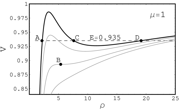
Figure 8: Effective potential outside of source for the third member of the family of Morgan and Morgan disks, $n=2$, for a timelike geodesic with $\mu=1$.

The behavior of the effective potential for different values of parameters is similar to that we displayed in Fig. 5, corresponding to the timelike geodesic. In the effective potential of the Fig. 5 we put $\ell=8$, 6 (gray curve) and 3.56 (dotted curve). The behavior for different values of the parameters is similar, so we take $\mu=1$ as an example. In the exterior case we consider the third member of the family, $n=2$, Fig. 8. In this graph the point $B$ corresponds to the radius of the marginally stable circular orbit, which have $\ell\approx 3.688$. The points $C$ and $D$ have angular momentum $\ell=4.2$ and effective potential $0.935$, the motion is bounded between the radius $7.61$ and $19.14$, Fig. 9. In this graph we choose $\mu=1$.

V Solutions in Prolate Spheroidal Coordinates

The general static axisymmetric vacuum solution for $\psi$ in prolate spheroidal coordinates $(u,v)$ is given by Q1

$$\psi_{l}=\sum_{n=0}^{l}(-1)^{n+1}d_{n}Q_{n}(u)P_{n}(v),$$ (56)

where $u\geq 1$, $-1\leq v\leq 1$, and the $d_{n}$ are constants related with the multipole moments Q1 ; MA . $P_{n}$ are the Legendre polynomials and $Q_{n}$ are Legendre functions of second kind. These coordinates are related with Weyl’s canonical coordinates by

$$\rho^{2}=m^{2}(1-v^{2})(u^{2}-1),\qquad z=muv,$$ (57)

being $m$ the mass of the source that produce the field.

The asymptotically flat solution for $\gamma$ was found for Quevedo in Q1 . The monopolar solution, $l=0$, with $d_{0}=1$ corresponds to the Schwarzschild field. The solution of equation (16) for the monopolar solution is $u=2$, that is the unstable radius of a null circular orbit in the Schwarzschild field. For a complete study of motion in Schwarzschild field in the equatorial plane, see V1 . The solution of (56) for $l=2$ is the Erez-Rosen metric ER ,

$$\psi_{1} = \frac{d_{0}}{2}\ln\frac{u-1}{u+1}$$

$$+\frac{d_{2}}{2}(3v^{2}-1)\left[\frac{1}{4}(3u^{2}-1)\ln\frac{u-1}{u+1}+\frac{3}{2}u\right].$$

In this solution, $d_{0}$ and $d_{2}$ are related with the monopole and arbitrary quadrupole moment, respectively MA . The study of orbits in this solution was developed by different authors

Now, in this section we expose the expressions for the different quantities corresponding to the motion of a particle in a circular orbit in prolate spheroidal coordinates. That is, the specific energy, the angular velocity and the radius of the marginally stable circular orbit, which are obtained through of the effective potential in the equatorial plane,

$$V=e^{2\psi_{l}}\left(\epsilon^{2}+\frac{e^{2\psi_{l}}\ell^{2}}{\left(u^{2}-1\right)m^{2}}\right).$$

We begin with the equations corresponding to null geodesics, when $\epsilon=0$. So, the radius of the circular orbits can be determinate by

$$2(u^{2}-1)\psi_{l,\,u}=u,$$ (59)

that in terms of (56) takes the form

$$\sum_{n=0}^{l}2d_{2n}P_{2n}(0)(u^{2}-1)Q^{\prime}_{2n}(u)=u,$$ (60)

with the stability condition

$$u(u^{2}-1)\psi_{,uu}+(u^{2}+1)\psi_{,u}\geq 0,$$ (61)

that using (56) can be written as

$$\sum_{n=0}^{l}d_{2n}P_{2n}(0)\left[(u^{2}-1)Q^{\prime}_{2n}(u)-2nu(2n+1)Q_{2n}(u)\right]\geq 0,$$ (62)

where the equality corresponds to the equation for the radius of the marginally stable circular orbit. Finally, the other expressions are found by means of (14) and (27).

On the other hand, for the massive particle we obatin the expressions

$$\ell^{2} = \frac{e^{-2\psi}\left(u^{2}-1\right)^{2}m^{2}\psi_{,u}}{u-2\left(u^{2}-1\right)\psi_{,u}},$$ (63)

$$E^{2} = \frac{e^{2\psi}\left[u-(u^{2}-1)\psi_{,u}\right]}{u-2\left(u^{2}-1\right)\psi_{,u}},$$ (64)

where $u-2\left(u^{2}-1\right)\psi_{,u}\geq 0$ in order that the energy per mass unit and the angular moment per mass both be not imaginary. The stability condition and the radius of the marginally stable circular orbit are

$$\vspace{-1cm}\psi_{,u}\left\{3u^{2}+2+2(u^{2}-1)\psi_{,u}\left[2(u^{2}-1)\psi_{,u}-3u\right]\right\}$$

$$\ +\ u(u^{2}-1)\psi_{,uu}\geq 0,$$ (65)

with $u-2\left(u^{2}-1\right)\psi_{,u}\geq 0$.

Finally, we show in Fig. 10the region of stability by means of a graph of the specific angular moment (63). In particular, by taking arbitrary values of the parameters in the Erez-Rosen solution, one can see that the range is

$$0\leq u\leq 4.77,\qquad 4.77\leq u<\infty,$$

and $11.62\leq\ell<\infty$ for stable orbits, where we choose $d_{0}=1$ and $d_{2}=1.5$. Here the marginally stable circular orbit have coordinates $(\ell/m,u)=(11.62,4.77)$.

VI Concluding remarks

In this paper we analyzed the behavior of free test particles in the equatorial plane of static axisymmetric spacetimes. We presented several general expressions for the circular orbit in null and timelike geodesics: radius, specific energy, specific angular momentum, angular velocity and radius of the marginally stable circular orbit, all of them obtained through of an effective potential. The specific angular momentum was presented for the timelike geodesic and was used to determine the range of stability of the orbit of the particle, so the the minimum value represents the marginally stable circular motion.

In order to find the trajectory of the particle, we analyzed the analytical results obtained. The character of the motion is determined essentially by means of the behavior of the effective potential. Thus, we displayed different graphs of effective potential before resolve the differential equations of motion of the particle. Then, we began with the Chazy-Curson field in the case of the cylindrical coordinates, as discussed in section III. The motion of particles around oblate deformed bodies was developed in section IV, by means of the analysis of the properties of some member of the family disks (42). On the other hand, the prolate case was presented in section V, where we found the range of stability of the Erez-Rosen solution in the special case of mass particles.

In summary, we concluded that for these solutions all the circular orbits are unstable only in the case of null geodesic, whereas that do not exist marginally stable circular orbit for null geodesic. In contrast, we found that for mass particles the orbits can be unbounded, bounded or circular. This behavior can be seen by means of the effective potential and verified through the numerical solution of the equations of motion. Moreover, for the timelike geodesic we found the radius of the marginally stable circular orbit in different coordinate systems, cylindrical, prolate and oblate.

Figure 1: The effective potential for the massless particle in the Chazy-Curzon field. Here we take $\ell=4me$.

Figure 2: Effective potential as a function of $\rho/m$ for timelike geodesics, with different values of $\ell/m$, for the Chazy-Curzon field. For the curves from top to bottom we take $\ell/m=4.1,3.8,3.65$ and $\ell=3.52m$, respectively. The point in the dotted curve corresponds to $\rho/m=5.23$, which is the radius of the marginally stable orbit with $\ell/m=3.52$.

Figure 3: Effective potential for timelike geodesic with $\ell=4.5m$ in the Chazy- Curzon spacetimes.

Figure 4: Orbit of the particle corresponding to the effective potential of the Fig. 3 with $E_{1}=0.975$. This orbit is bounded between $C\approx 7.66$ and $D\approx 67.52$. The initial conditions are $\dot{\rho}(t=0)\approx 0.17$, $\varphi(t=0)=\pi/6$ and $\rho(t=0)=20$.

Figure 5: Orbit of the particle corresponding to the effective potential of the Fig. 3 with $E_{2}=1.02$. The initial conditions are $\dot{\rho}(t=0)\approx 0.17$, $\varphi=\pi/6$ and $\rho=20$.

Figure 6: The specific angular momentum, $\ell/m$, as a function of the radius of the circular orbit, $\rho/m$, for timelike geodesic in the Chazy-Curzon field. The point have coordinates $(\ell/m,\rho/m)=(3.52,5.23)$. The range of stability is $3.52m\leq\ell<\infty$ and $5.23m\leq\rho<\infty$.

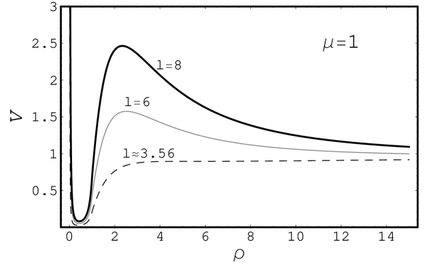
Figure 7: Effective potential inside and outside of the source for mass particles for the second member of the family of Morgan and Morgan disks, $n=1$, with $\mu=1$.

Figure 9: Orbit of a particle with $E=0.935$. The initial conditions are $\dot{\rho}(0)=0.0903$, $\varphi(0)=\pi/6$ and $\rho(0)=10$. The trajectory is between $C\leq\rho\leq D$.

Figure 10: Specific angular momentum, $\ell/m$, as a function of $u$ for the circular orbit in the Erez-Rosen field with $d_{0}=1$ and $d_{2}=1.5$.

- (1) D. Kramer, H. Stephani, E. Herlt, and M. Maccallum, Exact Solutions of Einstein’s Fields Equations. (Cambridge University Press, 2000).
- (2) J. M. Bardeen and S. A. Teukolsky, Ap. J. 178, 347 (1972).
- (3) A. Armenti, Celestial Mechanics and Dynamical Astronomy, 6, 383 (1972)
- (4) A. Armenti, International Journal Theoretical Physics, 16, 813 (1977);
- (5) H. Quevedo and L. Parkes, Gen. Relativ. Gravit. 21, 1047 (1989)
- (6) H. Quevedo and L. Parkes, Gen. Relativ. Gravit. 23, 495 (1991)
- (7) K.D. Krori and J.C. Sarmah, Gen. Relativ. Gravit. 23, 801 (1991)
- (8) O. Semerák, M. Žáček and T. Zellerin, Mon. Not. R. Astron. Soc., 308, 705 (1999).
- (9) J. Young and G. Menon, Gen. Relativ. Gravit. 32, 1 (2000);
- (10) E. Guéron and P. S. Letelier, Phys. Rev. E 66, 046611 (2002).
- (11) P. S. Letelier, Phys. Rev. D 68, 104002 (2003).
- (12) L. A. D’Afonseca, P. S. Letelier, and S. R. Oliveira, Class. Quantum Grav. 22 3803 (2004).
- (13) L. Herrera, Found. Phys. Lett. 18, 21-36 (2005).
- (14) F. L. Dubeibe, L. A. Pachón and J. D. Sanabría, Phys. Rev. D 75, 023008 (2007).
- (15) H. Weyl, Ann. Physik. 54, 1117 (1917).
- (16) H. Weyl, Ann. Physik. 59, 185 (1919).
- (17) J. Chazy, Bull. Soc. Math. France 52 17 (1924).
- (18) H.E.J. Curzon, Proc. London Math. Soc. 23 477 (1924).
- (19) H. Bateman, Partial differential equations of mthematical physics (1932), Cambridge U. P.
- (20) G. A. González and J. I. Reina, Mon. Not. R. Astron. Soc., 371, 1873 (2006).
- (21) A. J. Kalnajs, Ap. J. 175, 63 (1972).
- (22) J. F. Ramos, G. A. González and F.L. Suspes, Mon. Not. R. Astron. Soc., 371, 1873 (2008).
- (23) D.M. Zipoy, Journal Math. Phys. 7, 1137 (1966).
- (24) B.H. Vorhees, Phys. Rev. D 2, 2219 (1970).
- (25) W. A. Bonnor and A. Sackfield, Commun Math. Phys. 8, 338 (1968)
- (26) T. Morgan and L. Morgan, Phys. Rev. 183, 1097 (1969).
- (27) T. Morgan and L. Morgan L., Phys. Rev. 2, 2756 (1970)
- (28) O. Semerák, Class. Quantum Grav. 17, 3589 (2001).
- (29) H. Quevedo, Phys. Rev., 33, 334 (1986); H. Quevedo, Phys. Rev. D 39, 2904. (1989)
- (30) V.S. Manko, Class. Quantum Grav. 17, 1613 (1990).
- (31) S. L. Shapiro and S. A. Teukolsky, Black Hole White Dwarfs, and Neutron Stars (John Wyley & Sons, 1983); S. Chandrasekhar, The Mathematical Theory of Black Hole. (Oxford University Press, New York, 1998); E. F. Taylor and J. A. Wheeler, Exploring Black Hole Introduction to General Relativity. (Addison Wesley Longman, 2000).
- (32) G. Erez and N. Rosen, Bull. Res. Counc. Isr. 8F, 47 (1959).