An algorithm for decoherence analyses of lights through three-dimensional periodic microstructures

Abstract

A transfer-matrix algorithm is presented herein as a beginning to study the transmission characteristics of coherent light through three-dimensional periodic microstructures, in which the structures are treated as two-dimensional-layer stacks and multiple reflections are considered negligible. The spatial-correlated noise is further introduced layer by layer to realize the actual decoherence of the light and allows for statistical investigation of the partial spatially coherent optics in transparent mediums. Numerical analyses show comparable results to the Gaussian Schell model in free-space cases, indicating the validity of the algorithms.

I Introduction

Nanoscale structures have achieved novel functions in electro-optic devices such as optical filters, optical modulators, phase conjugated systems, optical attenuators, beam amplifiers, tunable lasers, holographic data storage and even as parts for optical logic systems ap1 ; ap2 ; ap3 ; ap4 ; ap5 ; ap6 ; ap7 ; ap8 ; ap9 ; ap10 ; ap11 ; ap12 ; ap13 ; ap14 over the last few decades. In contrast to the assumption of the ideal coherent (plane-wave) light in most theoretical studies op1 ; op2 ; op3 ; op4 ; op5 ; op6 ; op7 , the associated decoherence characteristics and intensity distribution of the light, e.g. by light-emitting diodes (LED) led1 ; led2 ; led3 , otherwise introduce another critical issue for both fundamental research and potential industrial applications. Motivated by these concerns and based on our previous study on coupled-wave theory op6 , we present a transfer-matrix algorithm as a beginning to study the propagation of coherent light through three-dimensional periodic microstructures. This work discretizes the structures into two-dimensional-layer stacks composed of isotropic or birefringent materials in an arbitrary order, and multiple reflections are considered negligible. By employing a concept similar to the Langevin dynamics in the finite difference method lang1 , a noise phase characterized with spatial correlations $\tau$ is further included layer by layer to mimic the actual decoherence of the light and allows for statistical investigation of the partial spatially coherent optics. Here, the correlation length $\tau$ of the noise is assumed to be larger than the wavelength of the incidence $\lambda$, because the intense decoherence (small $\tau$) causes strong scattering and the multiple reflections thereby cannot be ignored. The generation of the noise function is fulfilled by using a standard numerical technique based on the Fourier transform fft1 ; fft2 and is formulated in the appendix for the two-dimensional cases studied. Numerical analyses for the propagation of the free-space Gaussian beam and the diffractions of the beam incident through a liquid-crystal grating at different spatial decoherence show comparable results to the Gaussian Schell model PCB1 ; PCB2 and can validate this study.

II Theoretical formulae

This section neglects the multiple reflections and derives the transfer-matrix algorithm that is much easier to manipulate algebraically, yet accounts for the effects of the Fresnel refraction and the single reflection at the interfaces of the medium. The assumption of no multiple reflection is legitimate for most practical transparent materials. In what follows, a reformulation, including the noise phase of electromagnetic fields, is fulfilled to demonstrate the decoherence behaviors of the light.

II.1 Transfer matrix method by RCWA

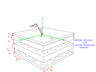
Figure 1: Geometry of three-dimensional RCWA algorithm for a multi-layer stack with two-dimensional periodic microstructures in arbitrary arrangement with isotropic and birefringent materials .

Referring to Figure 1, the structure is stratified along the medium normal into $N$ layers and these layers contribute to a total thickness of the stacks $Z_{N}=\sum_{\ell=1}^{N}z_{\ell}$. Each layer is considered as an arbitrary arrangement with homogeneous or birefringent materials, and the dielectric coefficients are generally described by a matrix:

$$\varepsilon=\left[\begin{array}[]{ccc}\varepsilon_{xx}&\varepsilon_{xy}&\varepsilon_{xz}\\ \varepsilon_{yx}&\varepsilon_{yy}&\varepsilon_{yz}\\ \varepsilon_{zx}&\varepsilon_{zy}&\varepsilon_{zz}\end{array}\right]$$ (1)

with

$$\varepsilon_{xx} = n_{o}^{2}+\left(n_{e}^{2}-n_{o}^{2}\right)\sin^{2}\theta_{o}\cos^{2}\phi_{o},$$

$$\varepsilon_{xy} = \varepsilon_{yx}=\left(n_{e}^{2}-n_{o}^{2}\right)\sin^{2}\theta_{o}\sin\phi_{o}\cos\phi_{o},$$

$$\varepsilon_{xz} = \varepsilon_{zx}=\left(n_{e}^{2}-n_{o}^{2}\right)\sin\theta_{o}\cos\theta_{o}\cos\phi_{o},$$

$$\varepsilon_{yy} = n_{o}^{2}+\left(n_{e}^{2}-n_{o}^{2}\right)\sin^{2}\theta_{o}\sin^{2}\phi_{o},$$

$$\varepsilon_{yz} = \varepsilon_{zy}=\left(n_{e}^{2}-n_{o}^{2}\right)\sin\theta_{o}\cos\theta_{o}\sin\phi_{o},$$

$$\varepsilon_{zz} = n_{o}^{2}+\left(n_{e}^{2}-n_{o}^{2}\right)\cos^{2}\theta_{o},$$ (2)

Here, $n_{e}$ and $n_{o}$ are extraordinary and ordinary indices of refraction of the uniaxially birefringent medium, respectively, $\theta_{o}$ is the angle between the optic axes and the $z$ axis, and $\phi_{o}$ is the angle between the projection of the optic axes on the $xy$ plane and $x$ axis.

To introduce the rigorous coupled-wave theory to the stack, all of the layers are defined as having the same periodicity: $\Lambda_{x}$ along the x direction and $\Lambda_{y}$ along the y direction. The periodic permittivity of an individual layer $\ell$ in the stack thereby can be expanded in the Fourier series of the spatial harmonics as:

$$\overline{\varepsilon}_{ij}\left(\overline{x},\overline{y},\overline{z}_{\ell}\right) = \sum_{g,h}\overline{\varepsilon}_{ij,gh}\left(\overline{z}_{\ell}\right)\exp\left(i\frac{g\lambda\overline{x}}{\Lambda_{x}}+i\frac{h\lambda\overline{y}}{\Lambda_{y}}\right)$$ (3)

$$\overline{\varepsilon}_{ij,gh}\left(\overline{z}_{\ell}\right) = \frac{\lambda}{2\pi\Lambda_{x}}\frac{\lambda}{2\pi\Lambda_{y}}\int_{0}^{\frac{2\pi\Lambda_{x}}{\lambda}}\int_{0}^{\frac{2\pi\Lambda_{y}}{\lambda}}\overline{\varepsilon}_{ij}\left(\overline{x},\overline{y},\overline{z}_{\ell}\right)\exp\left(-i\frac{g\lambda\overline{x}}{\Lambda_{x}}-i\frac{h\lambda\overline{y}}{\Lambda_{y}}\right)d\overline{x}d\overline{y}$$ (4)

Here, we have defined variables $k_{0}=\omega\sqrt{\mu_{0}\varepsilon_{0}}=\frac{2\pi}{\lambda}$, $Y_{0}=\frac{1}{Z_{0}}=\sqrt{\frac{\varepsilon_{0}}{\mu_{0}}}$, $\overline{r}=k_{0}r$, $\overline{x}=k_{0}x$, $\overline{y}=k_{0}y$, and $\overline{z}=k_{0}z$. $\lambda$ is the vacuum wavelength of the incident wave. Note that $\varepsilon_{ij\in\{x,y,z\}}$ are defined as functions of position ($x,y,z$) and $\overline{\varepsilon}_{ij}$ are defined for ($\overline{x},\overline{y},\overline{z}$). A parallel transform for the electromagnetic fields through the stack is expressed in terms of Rayleigh expansions:

$$\sqrt{Y_{0}}\mathbf{E}\left(\overline{x},\overline{y},\overline{z}_{\ell}\right) = \sum_{g,h}\mathbf{e}_{gh}\left(\overline{z}_{\ell}\right)\exp\left[-i\left(n_{xg}\overline{x}+n_{yh}\overline{y}\right)\right]$$ (5)

$$\sqrt{Z_{0}}\mathbf{H}\left(\overline{x},\overline{y},\overline{z}_{\ell}\right) = \sum_{g,h}\mathbf{h}_{gh}\left(\overline{z}_{\ell}\right)\exp\left[-i\left(n_{xg}\overline{x}+n_{yh}\overline{y}\right)\right]$$ (6)

$$n_{xg} = n_{I}\sin\theta\cos\phi-g\frac{\lambda}{\Lambda_{x}}$$ (7)

$$n_{yh} = n_{I}\sin\theta\sin\phi-h\frac{\lambda}{\Lambda_{y}}$$ (8)

This indicates the propagation of light along the direction $\mathbf{n_{gh}}=n_{xg}\hat{\imath}+n_{yh}\hat{\jmath}+\xi_{gh}\hat{k}$ with $\xi_{gh}=(n^{2}_{I(E)}-n_{yh}n_{yh}-n_{xg}n_{xg})^{1/2}$, in which $n_{I}$ and $n_{E}$ are the refraction index and correspond to the propagation in the incident and emitted regions, respectively. $\theta$, $\phi$ are the incident angles defined by sphere coordinates, and $z$ is the normal direction for the $xy$ plane of periodic structures.

Organizing the algorithms from our previous study op6 while ignoring the multiple reflections, the transfer-matrix formulae for the microstructure can thus be written as:

$$\left[\begin{array}[]{c}\vec{E}_{q,N+1}^{+}\\ \vec{M}_{q,N+1}^{+}\\ \vec{E}_{q,N+1}^{-}\\ \vec{M}_{q,N+1}^{-}\end{array}\right]=\mathbf{M}_{ext}\mathbf{M}_{N}...\mathbf{M}_{2}\mathbf{M}_{1}\mathbf{M}_{ent}\left[\begin{array}[]{c}\vec{E}_{q,0}^{+}\\ \vec{M}_{q,0}^{+}\\ \vec{E}_{q,0}^{-}\\ \vec{M}_{q,0}^{-}\end{array}\right]$$ (9)

Here, $\mathbf{M}_{i\in\{1\sim N\}}$ is the transfer matrix corresponding to the $i_{th}$ (anisotropic) structured layer. It is formulated by the eigen-vector matrix $\mathbf{T}^{(a)}_{i}$ with column eigen-vectors and the diagonal eigen-value matrix $\mathbf{\kappa}^{(a)}_{i}$ of the characteristic matrix $\mathbf{G}_{i}$ by:

$$\mathbf{M}_{i} = \mathbf{T}_{i}^{(a)}exp\left[i\mathbf{\kappa}_{i}^{a}\overline{z}_{i}\right](\mathbf{T}_{i}^{(a)})^{-1}$$ (10)

$$\mathbf{G}_{i} = \left[\begin{array}[]{cccc}\tilde{n}_{x}\tilde{\varepsilon}_{zz}^{-1}\tilde{\varepsilon}_{zx}&\tilde{n}_{x}\tilde{\varepsilon}_{zz}^{-1}\tilde{n}_{x}-1&\tilde{n}_{x}\tilde{\varepsilon}_{zz}^{-1}\tilde{\varepsilon}_{zy}&-\tilde{n}_{x}\tilde{\varepsilon}_{zz}^{-1}\tilde{n}_{y}\\ \tilde{\varepsilon}_{xz}\tilde{\varepsilon}_{zz}^{-1}\tilde{\varepsilon}_{zx}-\tilde{\varepsilon}_{xx}+\tilde{n}_{y}\tilde{n}_{y}&\tilde{\varepsilon}_{xz}\tilde{\varepsilon}_{zz}^{-1}\tilde{n}_{x}&\tilde{\varepsilon}_{xz}\tilde{\varepsilon}_{zz}^{-1}\tilde{\varepsilon}_{zy}-\tilde{\varepsilon}_{xy}-\tilde{n}_{y}\tilde{n}_{x}&-\tilde{\varepsilon}_{xz}\tilde{\varepsilon}_{zz}^{-1}\tilde{n}_{y}\\ \tilde{n}_{y}\tilde{\varepsilon}_{zz}^{-1}\tilde{\varepsilon}_{zx}&\tilde{n}_{y}\tilde{\varepsilon}_{zz}^{-1}\tilde{n}_{x}&\tilde{n}_{y}\tilde{\varepsilon}_{zz}^{-1}\tilde{\varepsilon}_{zy}&-\tilde{n}_{y}\tilde{\varepsilon}_{zz}^{-1}\tilde{n}_{y}+1\\ -\tilde{\varepsilon}_{yz}\tilde{\varepsilon}_{zz}^{-1}\tilde{\varepsilon}_{zx}+\tilde{\varepsilon}_{yx}+\tilde{n}_{x}\tilde{n}_{y}&-\tilde{\varepsilon}_{yz}\tilde{\varepsilon}_{zz}^{-1}\tilde{n}_{x}&-\tilde{\varepsilon}_{yz}\tilde{\varepsilon}_{zz}^{-1}\tilde{\varepsilon}_{zy}+\tilde{\varepsilon}_{yy}-\tilde{n}_{x}\tilde{n}_{x}&\tilde{\varepsilon}_{yz}\tilde{\varepsilon}_{zz}^{-1}\tilde{n}_{y}\end{array}\right]$$ (15)

where the notation $\vec{(.)}$ represents $N_{g}\times N_{h}$ vectors with components $(.)_{gh}$, $\tilde{n}_{x}$ ($\tilde{n}_{y}$) are $N_{g}N_{h}\times N_{g}N_{h}$ diagonal matrices with the diagonal elements $n_{xg}$ ($n_{yh}$), and $\tilde{\varepsilon}_{ij\in\{x,y,z\}}$ are $N_{g}N_{h}\times N_{g}N_{h}$ matrices with elements $\varepsilon_{ij,gh}$ formulated by $\vec{f}\sim\tilde{\varepsilon}_{ij}\vec{f^{\prime}}$ or $f_{gh}\sim\sum_{g^{\prime}h^{\prime}}\varepsilon_{ij,(g-g^{\prime})(h-h^{\prime})}f^{\prime}_{g^{\prime}h^{\prime}}$. $N_{g(h)}$ define the number of considered Fourier orders $g$ ($h$) in the $x$ ($y$) direction. $1$ is $N_{g}N_{h}\times N_{g}N_{h}$ identity matrix. One may understood that $(\mathbf{T}_{i}^{(a)})^{-1}$ term represents the coordinate transformation from the components of tangential fields $\mathbf{f}_{\hat{t},i}=[\vec{e}_{x,i}\ \vec{h}_{y,i}\ \vec{e}_{y,i}\ \vec{h}_{x,i}]^{t}$ at $i_{th}$ interface in Equations (5)-(6) into the independent components of the eigen-modes of the $i_{th}$ layer, $exp\left[i\mathbf{\kappa}_{i}^{a}\overline{z}_{i}\right]$ term then follows the corresponding eigen-mode transition lasting a distance $\overline{z}_{i}$, and $\mathbf{T}_{i}^{(a)}$ term is the inversely coordinate transformation back to the components of the tangential fields defining $\mathbf{f}_{\hat{t},i+1}$ at the next interface. The superscript $t$ indicates the matrix transposition. Summarily, $\mathbf{M}_{i}$ demonstrates the propagation of fields ($\mathbf{f}_{\hat{t},i}$ to $\mathbf{f}_{\hat{t},i+1}$) through the $i_{th}$ layer.

In the (isotropic) uniform incident ($i=0$) and emitted ($i=N+1$) regions, the eigen-modes are chosen as $\vec{E}_{q}^{+}$ and $\vec{M}_{q}^{+}$ ($\vec{E}_{q}^{-}$ and $\vec{M}_{q}^{-}$) op6 ; op7 , thereby representing the physical forward (backward) $TE$ and $TM$ waves, i.e. transverse electric and transverse magnetic fields corresponding to the plane of the diffraction wave, respectively. The transform between the eigen-modes and the tangential fields $\mathbf{f}_{\hat{t},0}=[\vec{e}_{x,0}\ \vec{h}_{y,0}\ \vec{e}_{y,0}\ \vec{h}_{x,0}]^{t}$ in the incident region ($i=0$) is written as:

$$\left[\begin{array}[]{c}\vec{e}_{x,0}\\ \vec{h}_{y,0}\\ \vec{e}_{y,0}\\ \vec{h}_{x,0}\end{array}\right] = \left[\begin{array}[]{cccc}\dot{\mathbf{n}}_{y}&\dot{\mathbf{n}}_{x}&\dot{\mathbf{n}}_{y}&\dot{\mathbf{n}}_{x}\\ \dot{\mathbf{n}}_{y}\mathbf{\xi}&\mathbf{\varepsilon_{I}\dot{\mathbf{n}}_{x}\xi}^{-1}&-\dot{\mathbf{n}}_{y}\mathbf{\xi}&-\mathbf{\varepsilon_{I}\dot{\mathbf{n}}_{x}\xi}^{-1}\\ -\dot{\mathbf{n}}_{x}&\dot{\mathbf{n}}_{y}&-\dot{\mathbf{n}}_{x}&\dot{\mathbf{n}}_{y}\\ \dot{\mathbf{n}}_{x}\mathbf{\xi}&-\mathbf{\varepsilon_{I}\dot{\mathbf{n}}_{y}\xi}^{-1}&-\dot{\mathbf{n}}_{x}\mathbf{\xi}&\mathbf{\varepsilon_{I}\dot{\mathbf{n}}_{y}\xi}^{-1}\end{array}\right]\left[\begin{array}[]{c}\vec{E}_{q,0}^{+}\\ \vec{M}_{q,0}^{+}\\ \vec{E}_{q,0}^{-}\\ \vec{M}_{q,0}^{-}\end{array}\right]$$ (28)

$$\equiv \mathbf{T}^{(i)}_{\varepsilon_{I}}\left[\begin{array}[]{c}\vec{E}_{q,0}^{+}\\ \vec{M}_{q,0}^{+}\\ \vec{E}_{q,0}^{-}\\ \vec{M}_{q,0}^{-}\end{array}\right]$$ (33)

Here, $\dot{\mathbf{n}}_{y}$ and $\dot{\mathbf{n}}_{x}$ are $N_{g}N_{h}\times N_{g}N_{h}$ diagonal matrices with normalized elements $\frac{n_{yh}}{m_{gh}}$ and $\frac{n_{xg}}{m_{gh}}$ respectively. $\mathbf{\xi}^{-1}$ is the matrix with elements $1/\xi_{gh}$ (not the inverse of the matrix $\mathbf{\xi}$), in which $m_{gh}=(n_{yh}n_{yh}+n_{xg}n_{xg})^{1/2}$, $\xi_{gh}=(\varepsilon_{I}-n_{yh}n_{yh}-n_{xg}n_{xg})^{1/2}$, and $\varepsilon_{I}=n_{I}^{2}$ have been defined for the incident region. A similar transform for $\mathbf{f}_{\hat{t},N+1}$ in the emitted region can be derived straightforwardly by replacing all the $\varepsilon_{I}$ in Equation (33) with $\varepsilon_{E}$ and can be obtained as $\mathbf{f}_{\hat{t},N+1}=\mathbf{T}^{(i)}_{\varepsilon_{E}}[\vec{E}_{q,N+1}^{+}\ \vec{M}_{q,N+1}^{+}\ \vec{E}_{q,N+1}^{-}\ \vec{M}_{q,N+1}^{-}]^{t}$, in which $\xi_{gh}=(\varepsilon_{E}-n_{yh}n_{yh}-n_{xg}n_{xg})^{1/2}$, and $\varepsilon_{E}=n_{E}^{2}$.

Moreover, $\mathbf{M}_{ent}$ is the matrix representing the light propagation from the incident region into the medium, and indicates the essential refraction and the reflection at the first interface of the medium. To consider these effects in a simple way, a virtual (isotropic) uniform layer, which has zero thickness and (scalar) average dielectric coefficient $\varepsilon_{a}=n^{2}_{avg}$, e.g. $n_{avg}=(n_{e}+n_{o})/2$ for the liquid-crystal grating, is assumed to exist between the incident region and the $1_{st}$ layer. $\mathbf{M}_{ent}$ thereby can be obtained as:

$$\mathbf{M}_{ent} = \mathbf{T}_{\mathbf{\varepsilon}_{a}}^{(i)}\left[\begin{array}[]{cc}\mathbf{W}_{1}^{-1}&\mathbf{0}\\ \mathbf{0}&\mathbf{0}\end{array}\right]$$ (36)

$$\left[\begin{array}[]{cc}\mathbf{W}_{1}&\mathbf{W}_{2}\\ \mathbf{W}_{3}&\mathbf{W}_{4}\end{array}\right] = \left[(\mathbf{T}_{\mathbf{\varepsilon}_{a}}^{(i)})^{-1}\mathbf{T}_{\mathbf{\varepsilon}_{I}}^{(i)}\right]^{-1}$$ (39)

Here, $\mathbf{T}_{\mathbf{\varepsilon}_{a}}^{(i)}$ is defined in Equation (33) with the replacements of $\varepsilon_{I}$ by $\varepsilon_{a}$, $\xi_{gh}=(\varepsilon_{a}-n_{yh}n_{yh}-n_{xg}n_{xg})^{1/2}$, and $\varepsilon_{a}=n_{avg}^{2}$. Parallel to the argument of $\mathbf{M}_{ent}$, another similar virtual (isotropic) uniform layer exists between the emitted region and the $N_{st}$ layer, and $\mathbf{M}_{ext}$ is approximated as:

$$\mathbf{M}_{ext} = \left[\begin{array}[]{cc}\mathbf{W}_{1}^{\prime-1}&\mathbf{0}\\ \mathbf{0}&\mathbf{0}\end{array}\right](\mathbf{T}_{\mathbf{\varepsilon}_{a}}^{(i)})^{-1}$$ (42)

$$\left[\begin{array}[]{cc}\mathbf{W}_{1}^{\prime}&\mathbf{W}_{2}^{\prime}\\ \mathbf{W}_{3}^{\prime}&\mathbf{W}_{4}^{\prime}\end{array}\right] = \left[(\mathbf{T}_{\mathbf{\varepsilon}_{E}}^{(i)})^{-1}\mathbf{T}_{\mathbf{\varepsilon}_{a}}^{(i)}\right]^{-1}$$ (45)

II.2 Algorithms extended for optical decoherences

To demonstrate the spatial decoherence of the light, the electric fields of an incident unit-amplitude plane wave are first denoted as:

$$\mathbf{E}\left(\mathbf{r}\right)=\mathbf{E}_{0}\exp\left[-i\mathbf{k}\cdot\mathbf{r}+i\eta\left(\mathbf{r}\right)\right]$$ (46)

The time dependence of $\exp\left(i\omega t\right)$ is assumed and omitted here. $\eta(x,y,z)$ is the noise phase of $\mathbf{E}$ and is conditioned by the correlation relation with a characteristic spatial coherent length $\tau$:

$$\left\langle\eta\left(\mathbf{r}\right)\eta\left(\mathbf{r}^{\prime}\right)\right\rangle = \gamma\left(\mathbf{r-r}^{\prime}\right)$$ (47)

$$= \pi^{2}\exp\left(-\frac{\left|\mathbf{r-r}^{\prime}\right|^{2}}{2\tau^{2}}\right)$$

with $\left\langle\eta\left(\mathbf{r}\right)\right\rangle=0$. The correlation function $\gamma\left(\mathbf{r-r}^{\prime}\right)$ is chosen as Gaussian distribution and describes a strong (weak) phase correlation between fields of closer (farther) positions than $\tau$. In the limit of $\tau\rightarrow\infty$, the $\eta\left(\mathbf{r}\right)$ is constant and the $\mathbf{E}$ field in Equation(46) shows the coherent incident wave, whereas in the limit of $\tau\rightarrow 0$, an incoherent (total random phase) wave is exhibited. Here, the generation of the noise function $\eta\left(\mathbf{r}\right)$ is fulfilled by using a standard numerical technique based on the Fourier transform and is formulated in the appendix for the two-dimensional cases studied. To realize the spatial decoherence analyses for the light, we introduce the concept similar to the Langevin dynamics for the stratified layers along the $z$ direction and include the noise phase layer by layer in Equation (9):

$$\left[\begin{array}[]{c}\vec{E}_{q,N+1}^{+}\\ \vec{M}_{q,N+1}^{+}\\ \vec{E}_{q,N+1}^{-}\\ \vec{M}_{q,N+1}^{-}\end{array}\right]=\mathbf{M}_{ext}\grave{\mathbf{R}}\mathbf{M}_{N}...\grave{\mathbf{R}}\mathbf{M}_{2}\grave{\mathbf{R}}\mathbf{M}_{1}\grave{\mathbf{R}}\mathbf{M}_{ent}\left[\begin{array}[]{c}\vec{E}_{q,0}^{+}\\ \vec{M}_{q,0}^{+}\\ \vec{E}_{q,0}^{-}\\ \vec{M}_{q,0}^{-}\end{array}\right]$$ (48)

Here, $\grave{\mathbf{R}}$ indicates the operations of three numerical processes on $\mathbf{f}_{\hat{t},i\in\{1\sim N+1\}}=\mathbf{M}_{i-1}...\grave{\mathbf{R}}\mathbf{M}_{2}\grave{\mathbf{R}}\mathbf{M}_{1}\grave{\mathbf{R}}\mathbf{M}_{ent}\cdot[\vec{E}_{q,0}^{+}\ \vec{M}_{q,0}^{+}\ \vec{E}_{q,0}^{-}\ \vec{M}_{q,0}^{-}]^{t}$ at $i_{th}$ interface by: (a) first fulfilling the inverse Fourier transform from the $k$ components of the tangential fields $\mathbf{f}_{\hat{t},i}(\bar{x},\bar{y})$ into the $r$ components, i.e. ($\sqrt{Y_{0}}\mathbf{E}$, $\sqrt{Z_{0}}\mathbf{H}$ ) by Equation (5); (b) next including the noise phase by multiplying the spatial $r$ components of the fields by the noise phase $e^{i\eta(x,y,z)}$, or $e^{i\eta(\bar{x},\bar{y},\bar{z})}$ in our work, as Equation (46); (c) and finally performing the Fourier transform on the $r$ components to obtain the $k$ components of the tangential fields $\mathbf{f}_{\hat{t},i}(\bar{x},\bar{y})$ including the noise phase. Hence, the field $\mathbf{f}_{\hat{t},i\in\{1\sim N+1\}}$ through the medium can approximately mimic decoherence behaviors by these processes.

III Numerical results for two-dimensional examples

To study the decoherence behavior of light, we first analyze the propagation of the Gaussian beam with different coherent lengths in a two-dimensional $xz$ free space, and fulfill a statistical numerical analysis over an ensemble of systems with 500 identical iterations. The characteristic period of the structure ($\Lambda_{x}=48\mu m$) is chosen to be much larger than the Gaussian beam profile ($\sim e^{-x^{2}/2\sigma^{2}}$ with $\sigma=6\mu m$) so that the periodic beam can be considered to be isolated in near-field optic analyses. The relevant parameters are given as: the x-grid size $\Delta_{x}=0.05\mu m$, the thickness of the stacked layer $z_{i\in\{1\sim N\}}=0.05\mu m$, the wavelength $\lambda=0.55\mu m$, the $y$-polarized incidence $\sqrt{Y_{0}}E_{y}(\bar{x},\bar{z}=0)=e^{-\bar{x}^{2}/2\sigma^{2}}$, the refraction indices $n_{I}=n_{E}=n_{o}=1.0\simeq n_{e}=1.0+10^{-5}$, and the Fourier order $-50<g<50$ ($h=0$). Figure 2 illustrates the intensity patterns $|\sqrt{Y_{0}}E_{y}(\bar{x},\bar{z})|^{2}+|\sqrt{Z_{0}}H_{x}(\bar{x},\bar{z})|^{2}$ of the free-space Gaussian beam with $\tau=5\mu m$, $\tau=1\mu m$, and $\tau=0.5\mu m$ along the light propagation. Figure 3 shows the corresponding numerical intensity to the Figure 2 after propagating a distance at $z=35\mu m$. The results indicate that the stronger decoherence (smaller $\tau$) of the light causes more a intense scattering along the propagation and shows comparable conclusion from the Gaussian Schell model PCB1 .

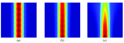
Figure 2: Intensity patterns of the free-space Gaussian beam with coherent length (a) $\tau=5\mu m$, (b) $\tau=1\mu m$, and (c) $\tau=0.5\mu m$ for the ensemble of 500 iterations in the $48\mu m\times 40\mu m$ $xz$ plane.

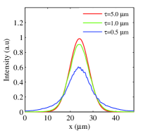
Figure 3: Numerical intensity of the Gaussian beam corresponding to the results of Figure 2 with $\tau=5\mu m$, $\tau=1\mu m$, and $\tau=0.5\mu m$ after propagating a distance at $z=35\mu m$.

To further investigate the decoherence behaviors of the light through the microstructures, a liquid-crystal grating film is included to introduce the diffraction of light. Figure 4 shows the one-period orientations of the liquid-crystals directors in a single-layer film. For this case, rather than employing the definition of the grating period $\Lambda_{x,LC}=1.2\mu m$ as in Figure 4, we apply SRC-RCWA scheme and set the characteristic period $\Lambda_{x}=48\mu m=24\times\Lambda_{x,LC}$. Hence, the long-range profile of the Gaussian beam in spatial space can be considered, and simultaneously the small-angle emittance of the beam ($\sim 1/\Lambda_{x}$) defined by the Fourier component in Equations (7)-(8) can be demonstrated. Figure 5 illustrates diffraction patterns $|\sqrt{Y_{0}}E_{y}(\bar{x},\bar{z})|^{2}+|\sqrt{Z_{0}}H_{x}(\bar{x},\bar{z})|^{2}$ of the beam incident through a forty-period liquid-crystal grating (enclosed by dashed lines) in $48\mu m\times 40\mu m$ $xz$ plane, in which the coherent lengths of the beam are statistically considered to be (a) $\tau=5\mu m$, (b) $\tau=1\mu m$, and (c) $\tau=0.5\mu m$ for an ensemble of 500 iterations. Figure 6 shows the corresponding numerical intensity of the beam to Figure 5 after propagating a distance at $z=35\mu m$. The results indicate that the coherent incidence ($\tau=5\mu m$) through gratings leads to definite diffractions as described in most studies op6 , while the decoherent one ($\tau=0.5\mu m$) exhibits an intense scattering similar to that in Figure 2(c) and Figure 3. The incidence with $\tau=1\mu m$ in Figure 5(b) and Figure 6 shows a simultaneous diffraction and scattering results and deviates from the results by the coherent optics.

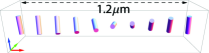
Figure 4: One-period orientations of liquid-crystal directors in the single-layer film, in which the red, green, and blue arrows indicate the spatial $\hat{x}$, $\hat{y}$, and $\hat{z}$ directions, respectively.

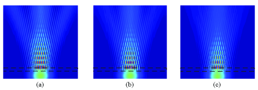
Figure 5: Intensity patterns of the Gaussian beam incident through a forty-period grating (dashed-line rectangle) in the $48\mu m\times 40\mu m$ $xz$ plane. The coherent lengths of the beam are statistically considered to be (a) $\tau=5\mu m$, (b) $\tau=1\mu m$, and (c) $\tau=0.5\mu m$ in an ensemble of 500 iterations.

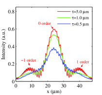
Figure 6: Numerical intensity of the Gaussian beam corresponding to the results of Figure 5 with $\tau=5\mu m$, $\tau=1\mu m$, and $\tau=0.5\mu m$ after propagating a distance at $z=35\mu m$.

IV Conclusions

This work has presented the formulas of the transfer-matrix method to conduct decoherence analyses in three-dimensional periodic microstructures. The algorithms are also devoted to doing a per-study of the light through turbid mediums that are related to the interaction between the fluctuated electron/dipole motions and the decoherence behaviors of light. Two numerical analyses for the propagation of free-space Gaussian beams and the diffraction of the liquid-crystal grating are then applied to verify the validity of this work, obtaining reasonable results.

V Acknowledgements

This work was supported in part by the National Science Council of the Republic of China under Contract Nos. NSC 99-2811-E-001-003 and NSC 98-2622-E-001-001-CC2.

Appendix A Generation of two-dimensional spatial correlated noises

In the following context, we introduce the generation of fluctuation function $\eta\left(\mathbf{r}\right)$ by the discrete Fourier method, and thereby realizing the $\mathbf{E}$ field describing partial coherence ($0<\tau<\infty$) in Equation (46). First, we introduce $\eta(\mathbf{k})$ in $2D$ momentum space, which follows the transforms of:

$$\eta\left(\mathbf{k}\right) = \int_{-\infty}^{\infty}\int_{-\infty}^{\infty}\eta\left(\mathbf{r}\right)\exp\left(-i\mathbf{k}\cdot\mathbf{r}\right)d\mathbf{r}$$ (49)

$$\eta\left(\mathbf{r}\right) = \frac{1}{4\pi^{2}}\int_{-\infty}^{\infty}\int_{-\infty}^{\infty}\eta\left(\mathbf{k}\right)\exp\left(i\mathbf{k}\cdot\mathbf{r}\right)d\mathbf{k}$$ (50)

or alternatively the discrete representation in $N\times N$ grid data under spatial interval $\Delta$ for our case

$$\eta_{g,h} = \Delta^{2}\sum_{u,v=0}^{N-1}\eta_{u,v}\exp\left[-i\frac{2\pi}{N}\left(g\cdot u+h\cdot v\right)\right],\text{ \ \ }g,h=0,1,...,N-1\text{\ \ }$$ (51)

$$\eta_{u,v} = \frac{1}{N^{2}\Delta^{2}}\sum_{g,h=0}^{N-1}\eta_{g,h}\exp\left[i\frac{2\pi}{N}\left(g\cdot u+h\cdot v\right)\right],\text{ \ \ }u,v=0,1,...,N-1$$ (52)

Here $u$, $v$ ($g$,$h$) are the indices for the spatial (momentum) space. The correlation function of the momentum space corresponding to that of the spatial space in Equation (47) is next derived as:

$$\left\langle\eta\left(\mathbf{k}\right)\eta\left(\mathbf{k}^{\prime}\right)\right\rangle = 4\pi^{2}\delta\left(\mathbf{k+k}^{\prime}\right)\gamma\left(\mathbf{k}\right)$$ (53)

$$= 4\pi^{2}\delta\left(\mathbf{k+k}^{\prime}\right)\cdot 2\pi^{3}\tau^{2}\exp\left[-\frac{1}{2}\mathbf{k}^{2}\tau^{2}\right]$$

where $\gamma\left(\mathbf{k}\right)$ is the Fourier transform of $\gamma\left(\mathbf{r}\right)$. The discrete representation of Equation (53) is

$$\left\langle\eta_{g,h}\eta_{g^{\prime},h^{\prime}}\right\rangle=N^{2}\Delta^{2}\gamma_{g,h}\delta_{g,N-g^{\prime}}\delta_{h,N-h^{\prime}}$$ (54)

Here, $\gamma_{g,h}$ is the discrete representation for $\gamma\left(\mathbf{k}\right)$ and exhibits the symmetry of $\gamma_{g,h}=\gamma_{N-g,h}=\gamma_{g,N-h}=\gamma_{N-g,N-h}$. Accordingly, by the discrete correlation equation in Equation (54), the fluctuation function $\eta_{g,h}$ can be generated in the discrete momentum space by:

$$\eta_{g,h}=N\Delta\sqrt{\gamma_{g,h}}\alpha_{g,h}$$ (55)

in which $\alpha_{g,h}$ is the Gaussian random number (complex number) with the average being zero, and it is conditioned as $\left\langle\alpha_{g,h}\alpha_{g^{\prime},h^{\prime}}\right\rangle=\delta_{g,N-g^{\prime}}\delta_{h,N-h^{\prime}}$, which corresponds to Equation (54). Definitely, these requirements for $\alpha_{g,h}$ can be realized by a simple process as:

$$\alpha_{0,0} = a_{0,0},\text{ \ \ \ }\alpha_{\frac{N}{2},\frac{N}{2}}=a_{\frac{N}{2},\frac{N}{2}}$$

$$\alpha_{\frac{N}{2},0} = b_{\frac{N}{2},0},\text{ \ \ \ }\alpha_{0,\frac{N}{2}}=b_{0,\frac{N}{2}}$$

$$\alpha_{g,0} = \frac{1}{\sqrt{2}}\left(a_{g,0}+ib_{g,0}\right),\text{ \ \ \ }\alpha_{N-g,0}=\frac{1}{\sqrt{2}}\left(a_{g,0}-ib_{g,0}\right)$$

$$\alpha_{0,h} = \frac{1}{\sqrt{2}}\left(a_{0,h}+ib_{0,h}\right),\text{ \ \ \ }\alpha_{0,N-h}=\frac{1}{\sqrt{2}}\left(a_{0,h}-ib_{0,h}\right)$$

$$\alpha_{g,\frac{N}{2}} = \frac{1}{\sqrt{2}}(a_{g,\frac{N}{2}}+ib_{g,\frac{N}{2}}),\text{ \ \ \ }\alpha_{N-g,\frac{N}{2}}=\frac{1}{\sqrt{2}}(a_{g,\frac{N}{2}}-ib_{g,\frac{N}{2}})$$

$$\alpha_{\frac{N}{2},h} = \frac{1}{\sqrt{2}}(a_{\frac{N}{2},h}+ib_{\frac{N}{2},h}),\text{ \ \ \ }\alpha_{\frac{N}{2},N-h}=\frac{1}{\sqrt{2}}(a_{\frac{N}{2},h}-ib_{\frac{N}{2},h})$$

$$\alpha_{g,h} = \frac{1}{\sqrt{2}}\left(a_{g,h}+ib_{g,h}\right),\text{ \ \ \ }\alpha_{N-g,N-h}=\frac{1}{\sqrt{2}}\left(a_{g,h}-ib_{g,h}\right)$$

$$\alpha_{g,N-h} = \frac{1}{\sqrt{2}}\left(a_{g,N-h}+ib_{g,N-h}\right),\text{ \ \ \ }\alpha_{N-g,h}=\frac{1}{\sqrt{2}}\left(a_{g,N-h}-ib_{g,N-h}\right)$$ (56)

Here, $a_{g,h}$ and $b_{g,h}$ are independent Gaussian random numbers (real numbers) with an average of zero and variance of one. Note that it is necessary to generate $N\times N$ independent Gaussian random numbers for $N\times N$ fluctuations of $\eta_{g,h}$.

Finally, $\eta_{u,v}$ in the discrete spatial space can be obtained straightforwardly by the Fourier transform of $\eta_{g,h}$ in Equation 52, such that the electric field $\mathbf{E}\left(x,z\right)=\mathbf{E}_{0}\exp\left[-i\mathbf{k}\cdot\mathbf{r}+\eta\left(x,z\right)\right]$ in the studied $xz$ region can be evaluated. A further treatment of $\eta_{u,v}\rightarrow\eta_{u,v}-\bar{\eta}$, in which $\bar{\eta}$ means the average noise over the $N\times N$ grid data, is executed to ensure the condition $\left\langle\eta\left(\mathbf{r}\right)\right\rangle=0$. It is straightforward to extend to arbitrary $N\times M$ periodic grid data. Numerical results of the noise phase with $\tau=5,1,0.5\mu m$ are illustrated in Figure 7 for reference.

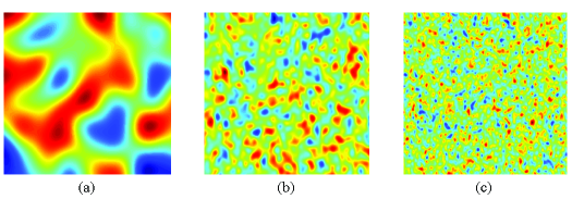
Figure 7: The noise phase $\eta(x,z)$ with (a) correlation length $\tau=5.0\mu m$, (b) correlation length $\tau=1.0\mu m$, and (c) correlation length $\tau=0.5\mu m$ in the studied $48\mu m\times 40\mu m$ $xz$ plane.

References

- (1) A. Miniewicz, S. Bartkiewicz, and J. Parka, Opt. Commun. 149, 89 (1998).
- (2) S. Bartkiewicz, A. Miniewicz, F. Kajzar, and M. Zagorska, Mol. Cryst. Liq. Cryst. 22, 213 (1999).
- (3) J. Mysliwiec, A. Miniewicz, and S. Bartkiewicz, Opto-Electron. Rev. 10, 53 (2002).
- (4) M. Bertolotti, G. Sansoni, and F. Scudieri, Appl. Opt. 18, 528 (1979).
- (5) L. M. Blinov, V. V. Lazarev, S. P. Palto, G. Cipparrone, A. Mazzulla, and P. Pagliusi, J. Nonlinear Opt. Phys. Mater. 16, 75 (2007).
- (6) A. Jacobson, J. Grinberg, W. Bleha, L. Miller, L. Fraas, G. Myer, and D. Boswell, Ann. New York Acad. Sci. 267, 417 (1975).
- (7) G. Labrunie, J. Robert, and J. Borel, Appl. Opt. 13, 1355 (1974).
- (8) S. Bartkiewicz, and A. Miniewicz, Adv. Mater. Opt. Electron. 6, 219 (1996).
- (9) J. Mysliwiec, and S. Bartkiewicz, K. Janus, Opt. Commun. 276, 58 (2008).
- (10) M. Sutkowski, T. Grudniewski, R. Zmijan, J. Parka, and E. N. Kruszelnicki, Opto-Electron. Rev. 14, 335 (2006).
- (11) F. Kajzar, S. Bartkiewicz, and A. Miniewicz, Appl. Phys. Lett. 74, 2924 (1999).
- (12) S. Bartkiewicz, P. Sikorski, and A. Miniewicz, Opt. Lett. 23, 1769 (1998).
- (13) B. K. Jenkins, A. A. Sawchuk, T. C. Strand, R. Forchheimer, and B. H. Soffer, Appl. Opt. 23, 3455 (1984).
- (14) L. M. Blinov, G. Cipparrone, P. Pagliusi, and S. L. Palto, Appl. Phys. Lett. 89, 031114 (2006).
- (15) B. Witzigmann, P. Regli, and W. Fichtner, J. Opt. Soc. Am. A. 15, 753 (1998).
- (16) E. E. Kriezis, S. K. Filippov, and S. J. Elston, J. Opt. A: Pure Appl. Opt. 2, 27 (2000).
- (17) K. Rokushima, and J. Yamakita, J. Opt. Soc. Am. 73, 901 (1983).
- (18) P. Galatola, C. Oldano, and P. B. Sunil Kumar, J. Opt. Soc. Am. A 11, 1332 (1994).
- (19) E. N. Glytsis, T. K. Gaylord, and J. Opt. Soc. Am. A 4, 2061 (1987).
- (20) I. L. Ho, Y. C. Chang, C. H. Huang, and W. Y. Li, Liq. Crys. 38, 241 (2011).
- (21) K. Rokushima, and J. Yamakita, J. Opt. Soc. Am. 73, 901 (1983).
- (22) D. S. Mehta, K. Saxena, S. K. Dubey, and C. Shakher, Journal of Luminescence 130, 96 V102 (2010).
- (23) F. J. Duarte, L.S. Liao, and K.M. Vaeth, Opt. Lett. 30, 3072 (2005).
- (24) F. J. Duarte, Opt. Lett. 32, 412 (2007).
- (25) C. Scherer, Braz. J. Phys. 34, 442 (2004).
- (26) J. Garcia-Ojalvo, and J. M. Sancho, Noise in Spatially Extended System, New York: Springer 1989.
- (27) J. Garcia-Ojalvo, and J. M. Sancho, L. R. Piscina, Phys. Rev. A 46, 4670 (1992).
- (28) X. Xiao, and D. Voelz, Optics Express 14, 6986 (2006).
- (29) P. Vahimaa, and J. Turunen, J. Opt. Soc. Am. A 14, 54 (1997).