Many-server queues with customer abandonment: Numerical analysis of their diffusion models

Abstract

We use multidimensional diffusion processes to approximate the dynamics of a queue served by many parallel servers. The queue is served in the first-in-first-out (FIFO) order and the customers waiting in queue may abandon the system without service. Two diffusion models are proposed in this paper. They differ in how the patience time distribution is built into them. The first diffusion model uses the patience time density at zero and the second one uses the entire patience time distribution. To analyze these diffusion models, we develop a numerical algorithm for computing the stationary distribution of such a diffusion process. A crucial part of the algorithm is to choose an appropriate reference density. Using a conjecture on the tail behavior of a limit queue length process, we propose a systematic approach to constructing a reference density. With the proposed reference density, the algorithm is shown to converge quickly in numerical experiments. These experiments also show that the diffusion models are good approximations for many-server queues, sometimes for queues with as few as twenty servers.

1104.0347 T1Supported in part by NSF Grants CMMI-0727400, CMMI-0825840, and CMMI-1030589. and

1 Introduction

The focus of this paper is the numerical analysis of multidimensional diffusion processes that approximate the dynamics of a queue with many parallel servers. A many-server queue serves as a building block modeling operations of a large-scale service system. Such a service system may be a call center with hundreds of agents, a hospital department with tens or hundreds of inpatient beds, or a computer cluster with many processors. When the customers of a service system are human beings, some of them may abandon the system before their service begins. The phenomenon of customer abandonment is ubiquitous because no one would wait for service indefinitely. As argued in Garnett, Mandelbaum and Reiman (2002), one must model customer abandonment explicitly in order for an operational model to be relevant for decision making. We model customer abandonment by assigning each customer a patience time. When a customer’s waiting time for service exceeds his patience time, he abandons the queue without service.

The exact analysis of such a many-server queue has been largely limited to an $M/M/n+M$ model (also called an Erlang-A model) that has a Poisson arrival process and exponential service and patience time distributions. See, e.g., Garnett, Mandelbaum and Reiman (2002). However, as pointed out by Brown et al. (2005), the service time distribution in a call center appears to follow a log-normal distribution. Such distributions have also been observed by Shi et al. (2010) for lengths of stay in a hospital. Moreover, the patience time distribution in a call center has been observed to be far from exponential by Zeltyn and Mandelbaum (2005). With a general service or patience time distribution, there is no finite-dimensional Markovian representation of the queue. Except computer simulations, there is no method to exactly analyze such a queue either analytically or numerically. To deal with the challenge, the following strategies are adopted in this paper for analyzing a many-server queue.

First, the service time distribution is restricted to be phase-type. Since phase-type distributions can be used to approximate any positive-valued distribution, such a queueing model is still relevant to practical systems. We focus on a $GI/Ph/n+GI$ queue with $n$ identical servers. The first $GI$ indicates that the customer interarrival times are independent and identically distributed (iid) following a general distribution, the $Ph$ indicates that the service times are iid following a phase-type distribution, and the $+GI$ indicates that the patience times are iid following a general distribution. Second, we are particularly interested in a queue operating in the Quality- and Efficiency-Driven (QED) regime: The queue has a large number of servers and the arrival rate is high; the arrival rate and the service capacity are approximately balanced so that the mean waiting time is relatively short compared with the mean service time. As argued in Garnett, Mandelbaum and Reiman (2002), such a system has high server utilization as well as short customer waiting times and a small fraction of abandonment. Therefore, both quality and efficiency can be achieved in this regime. Third, rather than analyzing the many-server queue itself, we propose and analyze diffusion models that approximate the queue. Two diffusion models are proposed in this paper. In each model, a multidimensional diffusion process is used to represent the scaled customer numbers among service phases. The difference between the two diffusion models lies in how the patience time distribution is built into them. The first diffusion model uses the patience time density at zero and the second one uses the entire patience time distribution. In particular, the diffusion process in the first model is a multidimensional piecewise Ornstein-Uhlenbeck (OU) process. We propose an algorithm in this paper to numerically solve the stationary distribution of a diffusion process. The computed stationary distribution is used to estimate the performance measures of a many-server queue. Numerical examples in Section 6 demonstrate that the diffusion models are very accurate in predicting the performance of a many-server queue, even if the queue has as few as twenty servers.

Except for the one-dimensional case, the stationary distribution of a piecewise OU process has no explicit formula. The algorithm proposed in this paper is a variant of the one in Dai and Harrison (1992), which computes the stationary distribution of a semimartingale reflecting Brownian motion (SRBM). As in Dai and Harrison (1992), the starting point of our algorithm is the basic adjoint relationship that characterizes the stationary distribution of a diffusion process. With an appropriate reference density, the algorithm can produce a stationary density that satisfies this relationship.

We set up a Hilbert space using the reference density. In this space, the stationary density is orthogonal to an infinite-dimensional subspace $H$. A finite-dimensional subspace $H_{k}$ is used to approximate $H$ and a function orthogonal to $H_{k}$ can be numerically computed by solving a system of finitely many linear equations. This function is used to approximate the stationary density. There are two sources of error in computing the approximate stationary density by our algorithm: approximation error and round-off error. The approximation error arises because $H_{k}$ is an approximation of $H$. As $H_{k}$ increases to $H$, the approximation error decreases to zero. The round-off error occurs because the solution to the system of linear equations has error due to the finite precision of a computer. As $H_{k}$ increases to $H$, the dimension of the linear system gets higher and the coefficient matrix becomes closer to singular. As a consequence, the round-off error increases. The condition number of the matrix is used as a proxy for the round-off error. Balancing the approximation error and the round-off error is an important issue in our algorithm.

A properly chosen reference density is essential for the convergence of the algorithm. By convergence, we mean that the approximation error converges to zero as $H_{k}$ increases to $H$. More importantly, a “good” reference density can make $H_{k}$ converge to $H$ quickly so that the resulting approximation error and round-off error are small simultaneously even though the dimension of $H_{k}$ is moderate. To ensure the convergence of the algorithm, the reference density should have a comparable or slower decay rate than the stationary density. Since the stationary density is unknown, we make a conjecture on the tail behavior of the limit queue length process of many-server queues with customer abandonment. We conjecture that the limit queue length process has a Gaussian tail and the tail depends on the service time distribution only through its first two moments. This tail is used to construct a product-form reference density. With this reference density, the algorithm appears to converge quickly, producing stable and accurate results. For comparison purposes, we also test the algorithm with a certain “naively” chosen reference density in Section 7.1. The algorithm fails to converge with the “naive” reference density. The major contributions of this paper are the proposed diffusion models and the proposed reference densities that are critical to the numerical algorithm for computing the stationary distribution of a diffusion model.

Our diffusion models are obtained by replacing certain scaled renewal processes by Brownian motions. The replacement procedure is rooted in the many-server heavy traffic limit theorems that are proved in an asymptotic regime. The two diffusion model proposed in this paper are motivated by the diffusion limits proved in Dai, He and Tezcan (2010) and Reed and Tezcan (2009). See Section 4.3 for more details. The theory of diffusion approximation for many-server queues can be traced back to the seminal paper by Halfin and Whitt (1981), where a diffusion limit was established for $GI/M/n$ queues. Garnett, Mandelbaum and Reiman (2002) proved a diffusion limit for $M/M/n+M$ queues that allows for customer abandonment, and Whitt (2005) generalized the result to $G/M/n+M$ queues. Puhalskii and Reiman (2000) established a diffusion limit for $GI/Ph/n$ queues. Their result was extended to $G/Ph/n+GI$ queues with customer abandonment in Dai, He and Tezcan (2010). Recently, Reed and Tezcan (2009) proved a diffusion limit for $GI/M/n+GI$ queues. In their framework, a refined limit process is obtained by scaling the patience time hazard rate function.

Harrison and Nguyen (1990) derived Brownian models for multiclass open queueing networks. Their diffusion models are SRBMs and are rooted in the conventional heavy traffic limit theorems that are pioneered in Iglehart and Whitt (1970) for serial networks and Reiman (1984) for single-class networks. See Williams (1996) for a survey of limit theorems in literature. For a two-dimensional SRBM living in a rectangle, Dai and Harrison (1991) proposed an algorithm computing its stationary distribution. Dai and Harrison (1992) extended the algorithm for an SRBM living in an orthant. To deal with the unbounded state space, the notion of a reference density was first introduced there. Their finite-dimensional space $H_{k}$ is constructed via (global) multinominals of order at most $k$. With this choice of $H_{k}$, the algorithm appears numerically unstable occasionally. In such a case, the round-off error may dominate the approximation error while the approximation error is still significant. Shen et al. (2002) extended Dai and Harrison (1991) to a hypercube state space of an arbitrary dimension. They used a finite element method to construct $H_{k}$ to avoid numerical instability. Their algorithm sometimes converges slowly because they did not explore a reference density. A linear programming algorithm for computing the stationary distribution of a diffusion process was proposed in Saure, Glynn and Zeevi (2009). Both SRBMs in an orthant and a diffusion approximation of many-server queues with two priority classes were investigated in their paper. Like the role of the reference density, it appears that the rescaling of variables is essential to the convergence of their algorithm.

The remainder of the paper is organized as follows. General diffusion processes are introduced in Section 2, where the basic adjoint relationship for a diffusion process is also presented. In Section 3, we begin with recapitulating the generic algorithm of Dai and Harrison (1992), and then propose a finite element implementation that follows Shen et al. (2002). Two diffusion models for $GI/Ph/n+GI$ queues are presented in Section 4. In Section 5, we discuss how to choose an appropriate reference density exploiting the tail behavior of a diffusion process. In Section 6, it is demonstrated via numerical examples that the diffusion models serve as good approximations of many-server queues. Section 7 is dedicated to some implementation issues arising from the proposed algorithm. The paper is concluded in Section 8. We leave the proofs of Propositions 2 and 3 to the appendix.

Notation

The symbols $\mathbb{N}$, $\mathbb{R}$, and $\mathbb{R}_{+}$ are used to denote the sets of positive integers, real numbers, and nonnegative real numbers, respectively. For $d,m\in\mathbb{N}$, $\mathbb{R}^{d}$ denotes the $d$-dimensional Euclidean space and $\mathbb{R}^{d\times m}$ denotes the space of $d\times m$ real matrices. We use $C_{b}^{2}(\mathbb{R}^{d})$ to denote the set of real-valued functions on $\mathbb{R}^{d}$ that are twice continuously differentiable with bounded first and second derivatives. For $z,w\in\mathbb{R}$, we set $z^{+}=\max\{z,0\}$, $z^{-}=\max\{-z,0\}$, and $z\wedge w=\min\{z,w\}$. All vectors are envisioned as column vectors. For a $d$-dimensional vector $x\in\mathbb{R}^{d}$, we use $x_{j}$ for its $j$th entry and $\operatorname*{diag}(x)$ for the $d\times d$ diagonal matrix with $j$th diagonal entry $x_{j}$. For a matrix $M$, $M^{\prime}$ denotes its transpose, $M_{ij}$ denotes its $(i,j)$th entry, and $|M|=(\sum_{i,j}M_{ij}^{2})^{1/2}$. We reserve $I$ for the $d\times d$ identity matrix, $e$ for the $d$-dimensional vector of ones, and $e^{j}$ for the $d$-dimensional vector with its $j$th entry one and all other entries zero. Given two functions $\varphi$ and $\hat{\varphi}$ from $\mathbb{N}$ to $\mathbb{R}$, we write $\hat{\varphi}(n)=O(\varphi(n))$ as $n\rightarrow\infty$ if there exists a constant $\kappa>0$ and some $n_{0}\in\mathbb{N}$ such that $|\hat{\varphi}(n)|\leq\kappa|\varphi(n)|$ for all $n>n_{0}$.

2 Diffusion processes

Let $d$ be a positive integer. This paper focuses on a $d$-dimensional diffusion process $X=\{X(t):t\geq 0\}$. Let $(\Omega,\mathcal{F},\mathbb{F},\mathbb{P})$ be a filtered probability space with filtration $\mathbb{F}=\{\mathcal{F}_{t}:t\geq 0\}$. We assume that $X$ satisfies the following stochastic differential equation

$$X(t)=X(0)+\int_{0}^{t}b(X(s))\,\mathrm{d}s+\int_{0}^{t}\sigma(X(s))\,\mathrm{d}B(s),$$ (2.1)

where the drift coefficient $b$ is a function from $\mathbb{R}^{d}$ to $\mathbb{R}^{d}$, the diffusion coefficient $\sigma$ is a function from $\mathbb{R}^{d}$ to $\mathbb{R}^{d\times m}$, and $B=\{B(t):t\geq 0\}$ is an $m$-dimensional standard Brownian motion with respect to $\mathbb{F}$. We assume that both $b$ and $\sigma$ are Lipschitz continuous, i.e., there exists a constant $c_{1}>0$ such that

$$\left|b(x)-b(y)\right|+\left|\sigma(x)-\sigma(y)\right|\leq c_{1}|x-y|\qquad\text{for all }x,y\in\mathbb{R}^{d}\text{.}$$ (2.2)

Under condition (2.2), the stochastic differential equation (2.1) has a unique strong solution, i.e., there exists a unique process $X$ on $(\Omega,\mathcal{F},\mathbb{F},\mathbb{P})$ such that (a) $X$ is adapted to $\mathbb{F}$, (b) for each sample path $\omega\in\Omega$, $X(t,\omega)$ is continuous in $t$, and (c) for each $t\geq 0$, the stochastic differential equation (2.1) holds with probability one. See Øksendal (2003) for more details. We also assume that $\sigma$ is uniformly elliptic, i.e., there exists a constant $c_{2}>0$ such that

$$y^{\prime}\Sigma(x)y\geq c_{2}y^{\prime}y\qquad\text{ for all }x,y\in\mathbb{R}^{d}\text{,}$$ (2.3)

where

$$\Sigma(x)=\sigma(x)\sigma^{\prime}(x).$$ (2.4)

We are interested in the diffusion processes that model the dynamics of a queue with many parallel servers. Parallel-server queues will be introduced in Section 4. In that section, two diffusion processes will be identified to model such a queue and the coefficients $b$ and $\sigma$ will be mapped out explicitly in terms of primitive data of the queue. The diffusion models presented in Section 4 are rooted in many-server heavy traffic limit theorems proved in Dai, He and Tezcan (2010) and Reed and Tezcan (2009).

A probability distribution $\pi$ on $\mathbb{R}^{d}$ is said to be a stationary distribution of $X$ if $X(t)$ follows distribution $\pi$ for each $t>0$ whenever $X(0)$ has distribution $\pi$. Condition (2.3) is required to ensure the uniqueness of the stationary distribution. See Dieker and Gao (2011) for more details. In this paper, we assume that $X$ has a unique stationary distribution $\pi$ and $\pi$ has a density $g$ with respect to the Lebesgue measure on $\mathbb{R}^{d}$. For a general diffusion process, there is no explicit solution for $\pi$. This paper develops a numerical algorithm computing $\pi$. As in Dai and Harrison (1992), the starting point of the algorithm is the basic adjoint relationship

$$\int_{\mathbb{R}^{d}}\mathcal{G}f(x)\,\pi(\mathrm{d}x)=0\qquad\text{for all }f\in C_{b}^{2}(\mathbb{R}^{d}),$$ (2.5)

where $\mathcal{G}$ is the generator of $X$ defined by

$$\mathcal{G}f(x)=\sum_{j=1}^{d}b_{j}(x)\frac{\partial f(x)}{\partial x_{j}}+\frac{1}{2}\sum_{j=1}^{d}\sum_{\ell=1}^{d}\Sigma_{j\ell}(x)\frac{\partial^{2}f(x)}{\partial x_{j}\partial x_{\ell}}\qquad\text{for each }f\in C_{b}^{2}(\mathbb{R}^{d})$$ (2.6)

and $\Sigma$ is the covariance matrix given by (2.4). The following theorem is a consequence of Proposition 9.2 in Ethier and Kurtz (1986).

Theorem 1.

Let $\pi$ be a probability distribution on $\mathbb{R}^{d}$ that satisfies (2.5). Then, $\pi$ is a stationary distribution of $X$.

In this paper, we conjecture that a stronger version of Theorem 1 is true.

Conjecture 2.

Let $\pi$ be a signed measure on $\mathbb{R}^{d}$ that satisfies (2.5) and $\pi(\mathbb{R}^{d})=1$. Then, $\pi$ is a nonnegative measure and consequently it is a stationary distribution of $X$.

Our algorithm is to construct a function $g$ on $\mathbb{R}^{d}$ such that

$$\int_{\mathbb{R}^{d}}g(x)\,\mathrm{d}x=1\qquad\text{and}\qquad\int_{\mathbb{R}^{d}}\mathcal{G}f(x)g(x)\,\mathrm{d}x=0\qquad\text{for all }f\in C_{b}^{2}(\mathbb{R}^{d})\text{.}$$ (2.7)

Assuming that Conjecture 2 is true, $g$ must be the unique stationary density of $X$. As a special case, the nonnegativity of a signed measure $\pi$ that satisfies (2.5) for a piecewise OU process was proposed as an open problem by Dai and Dieker (2010). Piecewise OU processes will be introduced in Section 4.3.1.

3 A finite element algorithm for stationary distributions

In this section, we propose a numerical algorithm computing the stationary density $g$. The basic algorithm follows the one developed in Dai and Harrison (1992). The finite element implementation closely follows Shen et al. (2002).

3.1 A reference density

To compute the stationary density $g$, we adopt a notion called a reference density that was first introduced by Dai and Harrison (1992). A reference density for $g$ is a function $r$ defined from $\mathbb{R}^{d}$ to $\mathbb{R}_{+}$ such that

$$\int_{\mathbb{R}^{d}}r(x)\,\mathrm{d}x<\infty\qquad\text{and\qquad}\int_{\mathbb{R}^{d}}q^{2}(x)r(x)\,\mathrm{d}x<\infty\text{,}$$ (3.1)

where

$$q(x)=\frac{g(x)}{r(x)}\qquad\text{for each }x\in\mathbb{R}^{d}$$

is called the ratio function. Such a function $r$ exists because $r=g$ is a reference density. The reference density controls the convergence of our algorithm. We will discuss how to choose a reference density for the diffusion models of a many-server queue in Section 5.

For the rest of Section 3, we assume that a reference density $r$ satisfying (3.1) has been determined and remains fixed. In addition, we assume that

$$\int_{\mathbb{R}^{d}}b_{j}^{2}(x)r(x)\,\mathrm{d}x<\infty\qquad\text{and}\qquad\int_{\mathbb{R}^{d}}\Sigma_{j\ell}^{2}(x)r(x)\,\mathrm{d}x<\infty$$ (3.2)

for $j,\ell=1,\ldots,d$. Since both $b$ and $\sigma$ are Lipschitz continuous, condition (3.2) is satisfied if

$$\int_{\mathbb{R}^{d}}\left|x\right|^{4}r(x)\,\mathrm{d}x<\infty.$$ (3.3)

Let $L^{2}(\mathbb{R}^{d},r)$ be the space of all square-integrable functions on $\mathbb{R}^{d}$ with respect to the measure that has density $r$, i.e.,

$$L^{2}(\mathbb{R}^{d},r)=\Big{\{}f\in\mathcal{B}(\mathbb{R}^{d}):\int_{\mathbb{R}^{d}}f^{2}(x)r(x)\,\mathrm{d}x<\infty\Big{\}}$$

where $\mathcal{B}(\mathbb{R}^{d})$ is the set of Borel-measurable functions on $\mathbb{R}^{d}$. Condition (3.1) implies that $q\in L^{2}(\mathbb{R}^{d},r)$. We define an inner product on $L^{2}(\mathbb{R}^{d},r)$ by

$$\langle f,\hat{f}\rangle=\int_{\mathbb{R}^{d}}f(x)\hat{f}(x)r(x)\,\mathrm{d}x\qquad\text{for }f,\hat{f}\in L^{2}(\mathbb{R}^{d},r)\text{.}$$

The induced norm is given by

$$\left\|f\right\|=\langle f,f\rangle^{1/2}\qquad\text{for each }f\in L^{2}(\mathbb{R}^{d},r)\text{.}$$ (3.4)

One can check that $L^{2}(\mathbb{R}^{d},r)$ is a Hilbert space and assumption (3.2) ensures that $\mathcal{G}f\in L^{2}(\mathbb{R}^{d},r)$ for all $f\in C_{b}^{2}(\mathbb{R}^{d})$. In $L^{2}(\mathbb{R}^{d},r)$, the basic adjoint relationship in (2.7) is equivalent to

$$\langle\mathcal{G}f,q\rangle=0\qquad\text{ for all }f\in C_{b}^{2}(\mathbb{R}^{d})\text{.}$$ (3.5)

With a fixed reference density $r$, we need only compute the ratio function $q$ by (3.5). Once $q$ is obtained, we can compute the stationary density via $g(x)=q(x)r(x)$ for $x\in\mathbb{R}^{d}$.

Let

$$H=\text{the closure of }\{\mathcal{G}f:f\in C_{b}^{2}(\mathbb{R}^{d})\}$$ (3.6)

where the closure is taken in the norm in (3.4). As a subspace of $L^{2}(\mathbb{R}^{d},r)$, $H$ is orthogonal to $q$. Let $c$ be a constant function and $c(x)=1$ for all $x\in\mathbb{R}^{d}$. Clearly, $c\in L^{2}(\mathbb{R}^{d},r)$ but $c\notin H$ because

$$\langle c,q\rangle=\int_{\mathbb{R}^{d}}g(x)\,\mathrm{d}x=1.$$ (3.7)

Let

$$\bar{c}=\operatorname*{arg\,min}_{f\in H}\left\|c-f\right\|$$ (3.8)

be the projection of $c$ onto $H$. Then, $c-\bar{c}$ must be orthogonal to $H$. Assuming that Conjecture 2 holds and $X$ has a unique stationary density $g$, one must have $q=\kappa_{q}(c-\bar{c})$ for some constant $\kappa_{q}\in\mathbb{R}$. By (3.7), the normalizing constant $\kappa_{q}$ satisfies

$$\kappa_{q}^{-1}=\langle c,c-\bar{c}\rangle=\langle c-\bar{c},c-\bar{c}\rangle+\langle\bar{c},c-\bar{c}\rangle=\left\|c-\bar{c}\right\|^{2}.$$

Hence, the ratio function is given by

$$q=\frac{c-\bar{c}}{\left\|c-\bar{c}\right\|^{2}}.$$ (3.9)

3.2 An approximate stationary density

To compute $q$ by (3.9), we need first compute $\bar{c}$, the projection of $c$ onto $H$. The space $H$ is linear and infinite-dimensional (i.e., a basis of $H$ contains infinitely many functions). In general, solving (3.8) in an infinite-dimensional space is impossible. In the algorithm, we use a finite-dimensional subspace $H_{k}$ to approximate $H$.

Suppose that there exists a sequence of finite-dimensional subspaces $\{H_{k}:k\in\mathbb{N}\}$ of $H$ such that $H_{k}\rightarrow H$ in $L^{2}(\mathbb{R}^{d},r)$ as $k\rightarrow\infty$. Here, $H_{k}\rightarrow H$ in $L^{2}(\mathbb{R}^{d},r)$ means that for each $f\in H$, there exists a sequence of functions $\{\varphi_{k}:k\in\mathbb{N}\}$ with $\varphi_{k}\in H_{k}$ such that $\left\|\varphi_{k}-f\right\|\rightarrow 0$ as $k\rightarrow\infty$. Let

$$\bar{c}_{k}=\operatorname*{arg\,min}_{f\in H_{k}}\left\|c-f\right\|$$

be the projection of $c$ onto $H_{k}$. By Proposition 7 of Dai and Harrison (1992), we have the following approximation result.

Proposition 1.

Assume that Conjecture 2 is true. Then,

$$\left\|q_{k}-q\right\|\rightarrow 0\qquad\text{as }k\rightarrow\infty\text{,}$$

where $q_{k}=(c-\bar{c}_{k})/\left\|c-\bar{c}_{k}\right\|^{2}$. Furthermore, when the reference density $r$ is bounded,

$$\int_{\mathbb{R}^{d}}(g_{k}(x)-g(x))^{2}\,\mathrm{d}x\rightarrow 0\qquad\text{as }k\rightarrow\infty\text{,}$$

where $g_{k}(x)=q_{k}(x)r(x)$ for each $x\in\mathbb{R}^{d}$.

As in Dai and Harrison (1992), we choose

$$H_{k}=\{\mathcal{G}f:f\in C_{k}\}$$ (3.10)

for some finite-dimensional space $C_{k}$. In Section 3.3, we will discuss how to construct $C_{k}$ using a finite element method. For notational convenience, we omit the subscript $k$ when $k$ is fixed. The finite-dimensional functional space is thus denoted by $C$. Let $m_{C}$ be the dimension of $C$ and $\{f_{i}:i=1,\ldots,m_{C}\}$ be a basis of $C$. We assume that the family $\{\mathcal{G}f_{i}:i=1,\ldots,m_{C}\}$ is linearly independent in $L^{2}(\mathbb{R}^{d},r)$. Then,

$$\bar{c}_{k}=\sum_{i=1}^{m_{C}}u_{i}\mathcal{G}f_{i}\qquad\text{for some }u_{i}\in\mathbb{R}\text{ and }i=1,\ldots,m_{C}\text{.}$$ (3.11)

Using the fact $\langle\mathcal{G}f_{i},c-\bar{c}_{k}\rangle=0$ for $i=1,\ldots,m_{C}$, we obtain a system of linear equations

$$Au=v$$ (3.12)

where

$$A_{i\ell}=\langle\mathcal{G}f_{i},\mathcal{G}f_{\ell}\rangle,\qquad u=(u_{1},\ldots,u_{m_{C}})^{\prime},\qquad v_{i}=\langle\mathcal{G}f_{i},c\rangle.$$ (3.13)

By the linear independence assumption, the $m_{C}\times m_{C}$ matrix $A$ is positive definite. Thus, $u=A^{-1}v$ is the unique solution to (3.12). Once the vector $u$ is obtained, we can compute the projection $\bar{c}_{k}$ by (3.11). Finally, the stationary density $g$ can be approximated via

$$g(x)\approx g_{k}(x)=r(x)\frac{c(x)-\bar{c}_{k}(x)}{\left\|c-\bar{c}_{k}\right\|^{2}}\qquad\text{for each }x\in\mathbb{R}^{d}\text{.}$$

3.3 A finite element method

In Dai and Harrison (1992), the authors employed multinominals of orders up to $k$ to construct the space $C_{k}$. This choice appears to be numerically unstable. The approximation error is significant when $k$ is small, say, $k\leq 5$. As $k$ increases, the round-off error in solving (3.12) increases and ultimately dominates the approximation error. Although their implementation produces accurate estimates for the stationary means of SRBMs, it sometimes produces poor estimates for the stationary distributions. In this section, we construct a sequence of spaces $\{C_{k}:k\in\mathbb{N}\}$ using the finite element method as in Shen et al. (2002). Because the state space in Shen et al. (2002) is bounded, neither a reference density nor state space truncation is used there.

The state space of $X$ is unbounded in our setting. It is necessary to truncate the state space to apply the finite element method. Let $\{K_{k}:k\in\mathbb{N}\}$ be a sequence of compact sets in $\mathbb{R}^{d}$. For each $f\in C_{k}$, we assume that $f(x)=0$ for $x\in\mathbb{R}^{d}\setminus K_{k}$. The subscript $k$ is omitted again when it is fixed and we use $K$ to denote the compact support of the space $C$. In our implementation, we restrict $K$ to be a $d$-dimensional hypercube

$$K=[-\zeta_{1},\xi_{1}]\times\cdots\times[-\zeta_{d},\xi_{d}],$$ (3.14)

where both $\zeta_{j}$ and $\xi_{j}$ are positive constants for $j=1,\ldots,d$.

We partition $K$ into a finite number of subdomains. Such a partition is called a mesh and each subdomain is called a finite element. Since $K$ is a hypercube, it is natural to use a lattice mesh, where each finite element is again a hypercube. In this case, each corner point of a finite element is called a node. In dimension $j=1,\ldots,d$, we divide the interval $[-\zeta_{j},\xi_{j}]$ into $n_{j}$ subintervals by partition points

$$-\zeta_{j}=y_{j}^{0}<y_{j}^{1}<\cdots<y_{j}^{n_{j}}=\xi_{j}.$$

Then, $K$ is divided into $\prod_{j=1}^{d}n_{j}$ finite elements. For future reference, we label the nodes in the way that node $(i_{1},\ldots,i_{d})$ corresponds to spatial coordinate $(y_{1}^{i_{1}},\ldots,y_{d}^{i_{d}})$, and define

$$h_{j}^{\ell}=y_{j}^{\ell+1}-y_{j}^{\ell}\qquad\text{for }\ell=0,\ldots,n_{j}-1\text{ and }j=1,\ldots,d\text{.}$$

If $\Delta$ denotes such a mesh, we define

$$\left|\Delta\right|=\max\{h_{j}^{\ell}:\ell=0,\ldots,n_{j}-1;\,j=1,\ldots,d\}$$

and

$$\eta_{\Delta}=\max\bigg{\{}\frac{h_{j_{1}}^{\ell_{1}}}{h_{j_{2}}^{\ell_{2}}}:\ell_{1},\ell_{2}=0,\ldots,n_{j}-1;\,j_{1},j_{2}=1,\ldots,d;\,\,j_{1}\neq j_{2}\bigg{\}}.$$ (3.15)

The finite-dimensional space $C$ is generated using the above mesh. We use the cubic Hermite basis functions to construct a basis of $C$, as in Shen et al. (2002). The one-dimensional Hermite basis functions for $-1\leq z\leq 1$ are given by

$$\phi(z)=(\left|z\right|-1)^{2}(2\left|z\right|+1)\qquad\text{and}\qquad\psi(z)=z(\left|z\right|-1)^{2}\text{.}$$ (3.16)

In dimension $j=1,\ldots,d$ and for $\ell=1,\ldots,n_{j}-1$, let

$$\phi_{j}^{\ell}(z)=\begin{cases}\phi\bigg{(}\dfrac{z-y_{j}^{\ell}}{h_{j}^{\ell-1}}\bigg{)}&\text{if }y_{j}^{\ell-1}\leq z\leq y_{j}^{\ell}\text{,}\\ \phi\bigg{(}\dfrac{z-y_{j}^{\ell}}{h_{j}^{\ell}}\bigg{)}&\text{if }y_{j}^{\ell}\leq z\leq y_{j}^{\ell+1}\text{,}\\ 0&\text{otherwise}\end{cases}$$

and

$$\psi_{j}^{\ell}(z)=\begin{cases}h_{j}^{\ell-1}\psi\bigg{(}\dfrac{z-y_{j}^{\ell}}{h_{j}^{\ell-1}}\bigg{)}&\text{if }y_{j}^{\ell-1}\leq z\leq y_{j}^{\ell}\text{,}\\ h_{j}^{\ell}\psi\bigg{(}\dfrac{z-y_{j}^{\ell}}{h_{j}^{\ell}}\bigg{)}&\text{if }y_{j}^{\ell}\leq z\leq y_{j}^{\ell+1}\text{,}\\ 0&\text{otherwise.}\end{cases}$$

Let $x=(x_{1},\ldots,x_{d})^{\prime}$ be a vector in $K$. At node $(i_{1},\ldots,i_{d})$, the basis functions of $C$ are the tensor-product Hermite basis functions

$$f_{i_{1},\ldots,i_{d},\chi_{1},\ldots,\chi_{d}}(x)=\prod_{j=1}^{d}g_{i_{j},\chi_{j}}(x_{j})$$ (3.17)

where $\chi_{j}$ is either $0$ or $1$ and

$$g_{i_{j},\chi_{j}}(z)=\begin{cases}\phi_{j}^{i_{j}}(z)&\text{if }\chi_{j}=0\text{,}\\ \psi_{j}^{i_{j}}(z)&\text{if }\chi_{j}=1\text{.}\end{cases}$$

Therefore, each node has $2^{d}$ tensor-product basis functions and the space $C$ has a total of

$$m_{C}=2^{d}\prod_{j=1}^{d}(n_{j}-1)$$ (3.18)

basis functions.

The space $C$ is not a subspace of $C_{b}^{2}(\mathbb{R}^{d})$. For the one-dimensional Hermite basis functions in (3.16), the second order derivative of $\phi(z)$ is not defined at $z=-1$ and $1$, and the second order derivative of $\psi(z)$ is not defined at $z=-1$, $0$, and $1$. As a consequence, there exists $f\in C$ for which $\mathcal{G}f$ is not defined on the boundaries of certain finite elements. Because such boundaries have Lebesgue measure zero in $\mathbb{R}^{d}$, for each $f\in C$, we can find a sequence of functions $\{\varphi_{i}:i\in\mathbb{N}\}$ in $C_{b}^{2}(\mathbb{R}^{d})$ such that $\left\|\mathcal{G}\varphi_{i}-\mathcal{G}f\right\|\rightarrow 0$ as $i\rightarrow\infty$. Hence, $H_{k}\subset H$ still holds for each $k$.

For the linear system (3.12) to have a unique solution, the family of functions

$$\{\mathcal{G}f_{i_{1},\ldots,i_{d},\chi_{1},\ldots,\chi_{d}}:i_{j}=1,\ldots,n_{j}-1;\chi_{j}=0,1;j=1,\ldots d\}$$

must be linearly independent in $L^{2}(\mathbb{R}^{d},r)$. The following proposition provides sufficient conditions for the linear independence. Its proof can be found in the appendix.

Proposition 2.

Let $\mathcal{G}$ be the generator of $X$ in (2.6) such that conditions (2.2) and (2.3) holds and all entries of $\Sigma$ are continuously differentiable. Assume that $r(x)>0$ for all $x\in\mathbb{R}^{d}$. Then, the family of functions

$$\{\mathcal{G}f_{i_{1},\ldots,i_{d},\chi_{1},\ldots,\chi_{d}}:i_{j}=1,\ldots,n_{j}-1;\chi_{j}=0,1;j=1,\ldots d\}$$

is linearly independent in $L^{2}(\mathbb{R}^{d},r)$, where $f_{i_{1},\ldots,i_{d},\chi_{1},\ldots,\chi_{d}}$ is the basis function of $C$ given by (3.17). Consequently, the solution to the linear system (3.12) is unique.

Now let us consider a sequence of functional spaces $\{C_{k}:k\in\mathbb{N}\}$. Let $\Delta_{k}$ be the mesh for constructing $C_{k}$. We assume that the mesh $\Delta_{k+1}$ is a refinement of $\Delta_{k}$, i.e., a node or an interelement boundary in $\Delta_{k}$ is also a node or an interelement boundary in $\Delta_{k+1}$. We further assume that such refinements are regular, i.e., for each $\eta_{\Delta_{k}}$ defined in (3.15), the set $\{\eta_{\Delta_{k}}:k\in\mathbb{N}\}$ is bounded. The next proposition, along with Proposition 1, justifies the proposed algorithm for computing the stationary distribution. We leave the proof of Proposition 3 to the appendix, too.

Proposition 3.

Let $\{\Delta_{k}:k\in\mathbb{N}\}$ be a sequence of lattice meshes such that each $\Delta_{k+1}$ is a refinement of $\Delta_{k}$ and the refinements are regular. Let $K_{k}$ be the $d$-dimensional finite hypercube that is the domain of $\Delta_{k}$, and $C_{k}$ be the functional space generated by $\Delta_{k}$ using the tensor-product Hermite basis functions in (3.17). Let $H$ be the infinite-dimensional space in (3.6) and $H_{k}$ be the finite-dimensional space in (3.10), where the generator $\mathcal{G}$ satisfies (2.2) and (3.2). Assume that

$$\left|\Delta_{k}\right|\rightarrow 0\qquad\text{and}\qquad K_{k}\uparrow\mathbb{R}^{d}\qquad\text{as }k\rightarrow\infty\text{.}$$

Then,

$$H_{k}\rightarrow H\qquad\text{as }k\rightarrow\infty\text{.}$$

4 Diffusion models for many-server queues

In this section, we introduce $GI/Ph/n+GI$ queues and present two diffusion models for such a queue with many servers. The two models differ in how the patience time distribution is built into them. The patience time density at zero is used in the first model, whereas the entire patience time distribution is used in the second model.

4.1 $GI/Ph/n+GI$ queues in the QED regime

We focus on a queue with many servers working in the QED regime. The QED regime will be discussed shortly. In this queue, the service time distribution is restricted to be phase-type. All positive-valued distributions can be approximated by phase-type distributions.

Let $p$ be a $d$-dimensional nonnegative vector whose entries sum to one, $\nu$ be a $d$-dimensional positive vector, and $P$ be a $d\times d$ sub-stochastic matrix. We assume that the diagonal entries of $P$ are zero and $P$ is transient, namely, $I-P$ is invertible. Consider a continuous-time Markov chain with $d+1$ phases (or states) where phases $1,\ldots,d$ are transient and phase $d+1$ is absorbing. For $j=1,\ldots,d$, the Markov chain starts in phase $j$ with probability $p_{j}$. The amount of time it stays in phase $j$ is exponentially distributed with mean $1/\nu_{j}$. When it leaves phase $j$, the Markov chain enters phase $\ell=1,\ldots,d$ with probability $P_{j\ell}$ or enters phase $d+1$ with probability $1-\sum_{\ell=1}^{d}P_{j\ell}$. The phase-type distribution with parameters $(p,\nu,P)$ is the distribution of time from starting until absorption in phase $d+1$ for the above Markov chain. In particular, when $P$ is a zero matrix, the associated phase-type distribution is a hyperexponential distribution with $d$ phases.

In a $GI/Ph/n+GI$ queue, there are $n$ identical servers working in parallel. The customer arrival process is a renewal process. Upon arrival, a customer enters service immediately if an idle server is available. Otherwise, he waits in a buffer with infinite waiting room that holds a first-in-first-out (FIFO) queue. The service times form a sequence of iid random variables, following a phase-type distribution. When a server finishes serving a customer, the server takes the leading customer from the waiting buffer. When the buffer is empty, the server begins to idle. Each customer has a patience time. The patience times are iid following a general distribution. When a customer’s waiting time in queue exceeds his patience time, the customer abandons the system with no service.

Let $\lambda$ be the arrival rate and $1/\mu$ be the mean service time. The system is assumed to operate in the QED regime, i.e., both the arrival rate $\lambda$ and the number of servers $n$ are large, while the traffic intensity $\rho=\lambda/(n\mu)$ is close to one. Because customer abandonment is allowed, it is not necessary to assume $\rho<1$ for the system to reach a steady state. For future purposes, we put

$$\beta=\sqrt{n}(1-\rho).$$ (4.1)

Assume that the phase-type service time distribution has parameters $(p,\nu,P)$. Each service time can be decomposed into a number of phases. When a customer is in service, he must be in one of the $d$ phases. Let $Z_{j}(t)$ denote the number of customers in phase $j$ service at time $t$. In steady-state, one expects that the customers in service are distributed among the $d$ phases following a distribution $\gamma$, given by

$$\gamma=\mu R^{-1}p\qquad\text{and}\qquad R=(I-P^{\prime})\operatorname{diag}(\nu)\text{.}$$ (4.2)

One can check that $\sum_{j=1}^{d}\gamma_{j}=1$ and $\gamma_{j}$ is interpreted to be the fraction of phase $j$ service load on the $n$ servers.

Suppose that all customers, including those initial customers waiting in the buffer at time zero, sample their first service phases following distribution $p$ upon arrival. One can stratify customers in the waiting buffer according to their first service phases. For $j=1,\ldots,d$, we use $W_{j}(t)$ to denote the number of waiting customers at time $t$ whose service begins with phase $j$. Then,

$$Y_{j}(t)=Z_{j}(t)+W_{j}(t)$$ (4.3)

is the number of phase $j$ customers in the system, either waiting or in service. Let $Y(t)$ be the corresponding $d$-dimensional random vector and

$$\tilde{Y}(t)=\frac{1}{\sqrt{n}}(Y(t)-n\gamma).$$ (4.4)

In each diffusion model, the process $\tilde{Y}=\{\tilde{Y}(t):t\geq 0\}$ is approximated by a $d$-dimensional diffusion process.

4.2 System equation

The $GI/Ph/n+GI$ queue is driven by several primitive processes. Let $E=\{E(t):t\geq 0\}$ be the arrival process, where $E(t)$ is the number of arrivals by time $t$. For $j=1,\ldots,d$, let $S_{j}=\{S_{j}(t):t\geq 0\}$ be a Poisson process with rate $\nu_{j}$, and $\phi_{j}=\{\phi_{j}(i):i\in\mathbb{N}\}$ be a sequence of iid $d$-dimensional random vectors such that $\phi_{j}(i)$ takes $e^{\ell}$ with probability $P_{j\ell}$ and takes a zero vector with probability $1-\sum_{\ell=1}^{d}P_{j\ell}$. Similarly, let $\phi_{0}=\{\phi_{0}(i):i\in\mathbb{N}\}$ be a sequence of iid $d$-dimensional random vectors such that $\phi_{0}(i)$ takes $e^{\ell}$ with probability $p_{\ell}$. For $j=0,\ldots,d$, define the routing process $\Phi_{j}=\{\Phi_{j}(k):k\in\mathbb{N}\}$ by

$$\Phi_{j}(k)=\sum_{i=1}^{k}\phi_{j}(i).$$

We assume that $Y(0),E,S_{1},\ldots,S_{d},\Phi_{0},\ldots,\Phi_{d}$ are mutually independent.

For $j=1,\ldots,d$, let $T_{j}(t)$ be the cumulative amount of service effort received by customers in phase $j$ service by time $t$. Clearly,

$$T_{j}(t)=\int_{0}^{t}Z_{j}(s)\,\mathrm{d}s\qquad\text{for }t\geq 0\text{.}$$ (4.5)

Thus, $S_{j}(T_{j}(t))$ is equal in distribution to the cumulative number of phase $j$ service completions by time $t$. (For more details, please refer to Section 4.1 of Dai, He and Tezcan (2010) on a perturbed system.) Let $L_{j}(t)$ be the cumulative number of phase $j$ customers who have abandoned the system by time $t$, and $L(t)$ be the corresponding $d$-dimensional vector. One can check that the process $Y=\{Y(t):t\geq 0\}$ satisfies the following equation

$$Y(t)=Y(0)+\Phi_{0}(E(t))+\sum_{j=1}^{d}\Phi_{j}(S_{j}(T_{j}(t)))-S(T(t))-L(t),$$ (4.6)

where $S(T(t))=(S_{1}(T_{1}(t)),\ldots,S_{d}(T_{d}(t)))^{\prime}$.

To derive the diffusion models, consider a scaled version of (4.6). We define several scaled processes by

$$\tilde{E}(t)=\frac{1}{\sqrt{n}}(E(t)-\lambda t),\qquad\tilde{S}(t)=\frac{1}{\sqrt{n}}(S(nt)-n\nu t),$$

$$\tilde{Z}(t)=\frac{1}{\sqrt{n}}(Z(t)-n\gamma,\qquad\tilde{L}(t)=\frac{1}{\sqrt{n}}L(t),)$$

$$\tilde{\Phi}_{0}(t)=\frac{1}{\sqrt{n}}\sum_{i=1}^{\left\lfloor nt\right\rfloor}(\phi_{0}(i)-p),\qquad\tilde{\Phi}_{j}(t)=\frac{1}{\sqrt{n}}\sum_{i=1}^{\left\lfloor nt\right\rfloor}(\phi_{j}(i)-p^{j})$$

for $t\geq 0$ and $j=1,\ldots,d$, where $p^{j}$ is the $j$th column of $P^{\prime}$. By (4.1)–(4.5), the dynamical equation in (4.6) turns out to be

$$\begin{split}\tilde{Y}(t)&=\tilde{Y}(0)-\beta\mu pt+p\tilde{E}(t)+\tilde{\Phi}_{0}\Big{(}\frac{E(t)}{n}\Big{)}\\ &\quad+\sum_{j=1}^{d}\tilde{\Phi}_{j}\Big{(}\frac{S_{j}(T_{j}(t))}{n}\Big{)}-(I-P^{\prime})\tilde{S}\Big{(}\frac{T(t)}{n}\Big{)}-R\int_{0}^{t}\tilde{Z}(s)\,\mathrm{d}s-\tilde{L}(t).\end{split}$$ (4.7)

4.3 Diffusion models

In both diffusion models, we replace the scaled primitive processes in (4.7) by certain Brownian motions. These approximations can be justified by the functional central limit theorem. When the number of servers $n$ is large, the corresponding diffusion process in each model can be proved close to $\tilde{Y}$ via a continuous map. Please refer to Dai, He and Tezcan (2010) for related convergence results.

Let $B_{E}$ be a one-dimensional driftless Brownian motion with variance $\lambda c_{a}^{2}/n$, where $c_{a}^{2}$ is the squared coefficient of variation for the interarrival time distribution. Let $B_{0},\ldots,B_{d}$, and $B_{S}$ are $d$-dimensional driftless Brownian motions with covariance matrices $H^{0},\ldots,H^{d}$, and $\operatorname*{diag}(\nu)$, respectively, where

$$H_{k\ell}^{0}=\begin{cases}p_{k}(1-p_{\ell})&\text{if }k=\ell\text{,}\\ -p_{k}p_{\ell}&\text{otherwise}\end{cases}$$

and

$$H_{k\ell}^{j}=\begin{cases}P_{jk}(1-P_{j\ell})&\text{if }k=\ell\text{,}\\ -P_{jk}P_{j\ell}&\text{otherwise}\end{cases}$$

for $j=1,\ldots,d$. We assume that $\tilde{Y}(0),B_{E},B_{0},\ldots,B_{d},B_{S}$ are mutually independent. In the diffusion models, the above Brownian motions take the places of the scaled primitive processes $\tilde{E},\tilde{\Phi}_{0},\ldots,\tilde{\Phi}_{d},\tilde{S}$, respectively. Let $Q(t)$ be the queue length or the number of waiting customers at time $t$ and

$$\tilde{Q}(t)=\frac{1}{\sqrt{n}}Q(t).$$

Then, $Q(t)=(e^{\prime}Y(t)-n)^{+}$ or equivalently,

$$\tilde{Q}(t)=(e^{\prime}\tilde{Y}(t))^{+}.$$ (4.8)

When $n$ is large, these waiting customers are approximately distributed among the $d$ phases according to distribution $p$ (see Lemma 2 of Dai, He and Tezcan (2010)), i.e.,

$$W_{j}(t)\approx p_{j}Q(t)\qquad\text{for }j=1,\ldots,d\text{.}$$

It follows from (4.3) that

$$Z(t)\approx Y(t)-pQ(t).$$

By (4.4) and (4.8), this approximation has a scaled version

$$\tilde{Z}(t)\approx\tilde{Y}(t)-p(e^{\prime}\tilde{Y}(t))^{+}.$$ (4.9)

Let $G(t)$ be the cumulative number of abandoned customers by time $t$ and

$$\tilde{G}(t)=\frac{1}{\sqrt{n}}G(t).$$

These abandoned customers are also approximately distributed among the $d$ phases by distribution $p$, i.e.,

$$\tilde{L}(t)\approx p\tilde{G}(t).$$ (4.10)

We also exploit the following approximations

$$\frac{E(t)}{n}\approx\frac{\lambda t}{n}=\rho\mu t,\qquad\frac{T(t)}{n}\approx(\rho\wedge 1)\gamma t,\qquad\frac{S_{j}(T_{j}(t))}{n}\approx(\rho\wedge 1)\nu_{j}\gamma_{j}t.$$ (4.11)

The approximations in (4.9)–(4.11) are used in both diffusion models. These two models differ only in how to approximate the scaled abandonment process $\tilde{G}=\{\tilde{G}(t):t\geq 0\}$.

4.3.1 Diffusion model using the patience time density at zero

In the first diffusion model, the patience time distribution is used only through its density at zero when approximating $\tilde{G}$. Let $F$ be the distribution function of the patience times. We assume that

$$F(0)=0\qquad\text{and}\qquad\alpha=\lim_{t\downarrow 0}\frac{F(t)}{t}<\infty\text{.}$$ (4.12)

Thus, $\alpha$ is the patience time density at zero. In this model, $\tilde{G}$ is approximated by

$$\tilde{G}(t)\approx\alpha\int_{0}^{t}(e^{\prime}\tilde{Y}(s))^{+}\,\mathrm{d}s\qquad\text{for }t\geq 0\text{.}$$ (4.13)

When $\alpha=0$, this approximation yields $\tilde{G}(t)\approx 0$ for all $t\geq 0$. In this case, the diffusion model is for a $GI/Ph/n$ queue without abandonment. When $\alpha>0$, the intuition of (4.13) is as follows. For a many-server queue in the QED regime, the queue length is typically in the order of $O(n^{1/2})$. As a result, each customer’s waiting time should be in the order of $O(n^{-1/2})$, which is relatively short because $n$ is large. At time $s$, a waiting customer will abandon the system during the next $\delta$ time units with probability $\alpha\delta$. Hence, the instantaneous abandonment rate of the system is approximately $\alpha Q(s)$. It follows that

$$G(t)\approx\alpha\int_{0}^{t}Q(s)\,\mathrm{d}s,$$

which, along with (4.4) and (4.8), leads to the approximation in (4.13). This relationship can be justified by Theorem 1 of Dai and He (2010). As pointed out by Dai and He (2010) and Mandelbaum and Momčilović (2009), the performance of a many-server queue in the QED regime is insensitive to the patience time distribution as long as its density $\alpha$ at zero is fixed and positive.

In the dynamical equation (4.7), when the scaled primitive processes are replaced by appropriate Brownian motions and the approximations in (4.9)–(4.13) are employed, we obtain the following stochastic differential equation

$$\begin{split}X(t)&=X(0)-\beta\mu pt+pB_{E}(t)+B_{0}(\rho\mu t)+\sum_{j=1}^{d}B_{j}((\rho\wedge 1)\nu_{j}\gamma_{j}t)\\ &\quad-(I-P^{\prime})B_{S}((\rho\wedge 1)\gamma t)-R\int_{0}^{t}(X(s)-p(e^{\prime}X(s))^{+})\,\mathrm{d}s\\ &\quad-p\alpha\int_{0}^{t}(e^{\prime}X(s))^{+}\,\mathrm{d}s\end{split}$$ (4.14)

where we take $X(0)=\tilde{Y}(0)$. We may write (4.14) into the standard form

$$X(t)=X(0)+\int_{0}^{t}b(X(s))\,\mathrm{d}s+\int_{0}^{t}\sigma(X(s))\,\mathrm{d}B(s),$$

where for each $x\in\mathbb{R}^{d}$, the drift coefficient $b$ is

$$b(x)=-\beta\mu p-R(x-p(e^{\prime}x)^{+})-p\alpha(e^{\prime}x)^{+},$$ (4.15)

the diffusion coefficient $\sigma$ is a $d\times d$ constant matrix satisfying

$$\begin{split}\Sigma(x)&=\sigma(x)\sigma^{\prime}(x)\\ &=\rho\mu(c_{a}^{2}pp^{\prime}+H^{0})\\ &\quad+(\rho\wedge 1)\bigg{(}\sum_{j=1}^{d}\nu_{j}\gamma_{j}H^{j}+(I-P^{\prime})\operatorname*{diag}(\nu)\operatorname*{diag}(\gamma)(I-P)\bigg{)},\end{split}$$ (4.16)

and $B$ is a $d$-dimensional standard Brownian motion. One can check that $\Sigma(x)$ is positive definite and thus satisfies (2.3). The drift coefficient $b$ in (4.15) is a piecewise linear function of $x$. Both $b$ and $\sigma$ are Lipschitz continuous. Therefore, a strong solution to (4.14) exists and is known as a $d$-dimensional piecewise OU process. In this model, the diffusion process $X$ depends on the patience time distribution only through its density at zero. When using the proposed algorithm to solve the stationary density, it follows from Proposition 2 that the linear system (3.12) has a unique solution.

If we replace $\rho$ by one in (4.14), the resulting diffusion process turns out to be the diffusion limit for $G/Ph/n+GI$ queues in Theorem 2 of Dai, He and Tezcan (2010). This limit process is the strong solution of the following stochastic differential equation

$$\begin{split}\check{X}(t)&=\check{X}(0)-\beta\mu pt+pB_{E}(t)+B_{0}(\mu t)+\sum_{j=1}^{d}B_{j}(\nu_{j}\gamma_{j}t)\\ &\quad-(I-P^{\prime})B_{S}(\gamma t)-R\int_{0}^{t}(\check{X}(s)-p(e^{\prime}\check{X}(s))^{+})\,\mathrm{d}s\\ &\quad-p\alpha\int_{0}^{t}(e^{\prime}\check{X}(s))^{+}\,\mathrm{d}s.\end{split}$$ (4.17)

Since $\rho$ is close to one in the current setting, the above limit process justifies the diffusion model in (4.14).

4.3.2 Diffusion model using patience time hazard rate scaling

When the patience time distribution does not have a density at zero, the diffusion model in (4.14) fails to exist. When $\alpha=0$ and $\rho>1$, the diffusion process $X$ in (4.14) does not have a stationary distribution. In this case, the model cannot be a satisfactory approximation of the many-server queue, as the queue may have a stationary distribution thanks to customer abandonment. It is also demonstrated in Reed and Tezcan (2009) that when the density near zero rapidly changes, the system performance can be sensitive to the patience time distribution in a neighborhood of the origin. In this case, using the patience time density at zero solely may not yield adequate approximation to the queue. Our second diffusion model exploits the idea of scaling the patience time hazard rate function, which was first proposed in Reed and Ward (2008) for single-server queues and was recently extended to many-server queues in Reed and Tezcan (2009).

In this model, we assume that the patience time distribution $F$ satisfies

$$F(0)=0$$

and it has a bounded hazard rate function $h$, given by

$$h(t)=\frac{f_{F}(t)}{1-F(t)}\qquad\text{for }t\geq 0\text{,}$$

where $f_{F}$ is the density of $F$. With the hazard rate function, $F$ can be written by

$$F(t)=1-\exp\Big{(}-\int_{0}^{t}h(s)\,\mathrm{d}s\Big{)}\qquad\text{for }t\geq 0\text{.}$$

In the second diffusion model, the scaled abandonment process $\tilde{G}$ is approximated by

$$\tilde{G}(t)\approx\int_{0}^{t}\int_{0}^{(e^{\prime}\tilde{Y}(s))^{+}}h\Big{(}\frac{\sqrt{n}u}{\lambda}\Big{)}\,\mathrm{d}u\,\mathrm{d}s\qquad\text{for }t\geq 0\text{.}$$ (4.18)

The entire patience time distribution is built into the approximation through its hazard rate function. The intuition of the hazard rate scaling approximation was explained in Reed and Ward (2008): Consider the $Q(s)$ waiting customers in the buffer at time $s$. In general, only a small fraction of customers can abandon the system when the queue is working in the QED regime. Then by time $s$, the $i$th customer from the back of the queue has been waiting around $i/\lambda$ time units. Approximately, this customer will abandon the queue during the next $\delta$ time units with probability $h(i/\lambda)\delta$. It follows that for the system, the instantaneous abandonment rate at time $s$ is close to $\sum_{i=1}^{Q(s)}h(i/\lambda)$. By (4.4) and (4.8), the scaled abandonment rate can be approximated by

$$\frac{1}{\sqrt{n}}\sum_{i=1}^{Q(s)}h\Big{(}\frac{i}{\lambda}\Big{)}\approx\int_{0}^{\tilde{Q}(s)}h\Big{(}\frac{\sqrt{n}u}{\lambda}\Big{)}\,\mathrm{d}u=\int_{0}^{(e^{\prime}\tilde{Y}(s))^{+}}h\Big{(}\frac{\sqrt{n}u}{\lambda}\Big{)}\,\mathrm{d}u,$$ (4.19)

from which (4.18) follows. Note that the arrival rate $\lambda$ is in the order of $O(n)$ and $Q(s)$ is in the order of $O(n^{1/2})$. The patience time distribution in a small neighborhood of zero, not just its density at zero, is considered in the instantaneous abandonment rate in (4.19). Hence, the hazard rate scaling approximation in (4.18) is more accurate than that in (4.13). This approximation can be justified for $GI/M/n+GI$ queues by Propositions 9.1 and 9.2 in Reed and Tezcan (2009). With minor modifications to the proofs, these two propositions can be extended to $GI/Ph/n+GI$ queues.

Let $m$ be a nonnegative integer. Suppose that the hazard rate function $h$ is $m$ times continuously differentiable in a neighborhood of zero. By Taylor’s theorem,

$$h(z)\approx h(0)+\sum_{\ell=1}^{m}h^{(\ell)}(0)\frac{z^{\ell}}{\ell!}$$

for $z>0$ small enough, where $h^{(\ell)}$ is the $\ell$th order derivative of $h$. In this case, the approximation in (4.18) turns out to be

$$\tilde{G}(t)\approx h(0)\int_{0}^{t}(e^{\prime}\tilde{Y}(s))^{+}\,\mathrm{d}s+\sum_{\ell=1}^{m}\frac{n^{\ell/2}h^{(\ell)}(0)}{\lambda^{\ell}(\ell+1)!}\int_{0}^{t}((e^{\prime}\tilde{Y}(s))^{+})^{\ell+1}\,\mathrm{d}s.$$

Because $h(0)$ is identical to the patience time density at zero, the approximation in (4.13) can be regarded as the zeroth degree Taylor’s approximation of (4.18). When the patience times are exponentially distributed, the hazard rate function is constant and the two approximations in (4.13) and (4.18) are identical. See Section 4 of Reed and Tezcan (2009) for more discussion.

Using the Brownian motion replacement and the approximations in (4.9)–(4.11) and (4.18), we obtain the second diffusion model for the $GI/Ph/n+GI$ queue, given by

$$\begin{split}X(t)&=X(0)-\beta\mu pt+pB_{E}(t)+B_{0}(\rho\mu t)+\sum_{j=1}^{d}B_{j}((\rho\wedge 1)\nu_{j}\gamma_{j}t)\\ &\quad-(I-P^{\prime})B_{S}((\rho\wedge 1)\gamma t)-R\int_{0}^{t}(X(s)-p(e^{\prime}X(s))^{+})\,\mathrm{d}s\\ &\quad-p\int_{0}^{t}\int_{0}^{(e^{\prime}X(s))^{+}}h\Big{(}\frac{\sqrt{n}u}{\lambda}\Big{)}\,\mathrm{d}u\,\mathrm{d}s.\end{split}$$ (4.20)

The diffusion process $X$ in (4.20) has the same diffusion coefficient $\sigma$ as in the first model (4.14). Its drift coefficient $b$ is

$$b(x)=-\beta\mu p-R(x-p(e^{\prime}x)^{+})-p\int_{0}^{(e^{\prime}x)^{+}}h\Big{(}\frac{\sqrt{n}u}{\lambda}\Big{)}\,\mathrm{d}u\qquad\text{for }x\in\mathbb{R}^{d}\text{.}$$ (4.21)

Because $h$ is bounded, the drift coefficient $b$ is Lipschitz continuous and the stochastic differential equation (4.20) has a strong solution. By Proposition 2, the solution to the linear system (3.12) is unique when we use the proposed algorithm to solve the stationary density of this diffusion model. Comparing (4.14) and (4.20), one can see that the two models differ only in how the patience time distribution is incorporated. Because a more accurate approximation is used for the abandonment process, the second model can provide a better approximation for the queue.

5 Choosing a reference density

The reference density controls the convergence of the proposed algorithm. In this section, we discuss how to choose appropriate reference densities for the diffusion models. Some considerations are as follows.

First, to be a reference density, a candidate function $r$ must satisfy (3.1) even though the stationary density $g$ is unknown. The second condition in (3.1) requires that $r$ have a comparable or slower decay rate than $g$. When $g$ is bounded, its decay rate is sufficient to determine a function $r$ that satisfies (3.1).

Second, the most computational effort in the algorithm is constructing and solving the system of linear equations (3.12). As demonstrated by Proposition 3, the finite-dimensional $H_{k}$ approximates the infinite-dimensional $H$ better as $k$ increases, thus reducing the approximation error. On the other hand, as the dimension of $H_{k}$ increases, constructing and solving (3.12) requires more computation time and memory space. The condition number of the matrix $A$ in (3.12) also gets worse as the dimension of $H_{k}$ becomes large. This yields higher round-off error. A “good” reference density should balance the approximation error and the round-off error. With such a reference density, it is possible to have small approximation error even if the dimension of $H_{k}$ is moderate.

Intuitively, when $r$ is “close” to the stationary density $g$, both the ratio function $q$ and the projection $\bar{c}$ are close to constant. We can thus expect that a space $H_{k}$ with a moderate dimension is able to produce a satisfactory approximation. All these observations motivate us to explore the tail behavior of a diffusion model.

5.1 Tail behavior

Let us focus on the diffusion limit in (4.17). Assume that the piecewise OU process $\check{X}$ is positive recurrent and has a stationary distribution. Let $\check{X}(\infty)$ be the corresponding $d$-dimensional random vector in steady state. Since $\rho$ is close to one, the tail behavior of the diffusion process $X$ in (4.14) is expected to be comparable to that of the limit diffusion process $\check{X}$ in (4.17).

To explore the tail behavior of $\check{X}(\infty)$, consider a sequence of $GI/GI/n+GI$ queues in the QED regime. If all patience times are infinite, the queues turn out to be $GI/GI/n$ queues without customer abandonment. In each queue, the service times are iid following a general distribution. We assume that these queues, each indexed by the number of servers $n$, have the same service time distribution. Let $\lambda_{n}$ be the arrival rate of the $n$th system. To mathematically define the QED regime, we assume that

$$\lim_{n\rightarrow\infty}\frac{\lambda_{n}}{n}>0$$ (5.1)

and

$$\lim_{n\rightarrow\infty}\sqrt{n}(1-\rho_{n})=\check{\beta}\qquad\text{for some }\check{\beta}\in\mathbb{R}\text{,}$$ (5.2)

where $\rho_{n}=\lambda_{n}/(n\mu)$ is the traffic intensity of the $n$th system.

Assume that all these queues are in steady state. Let $N_{n}(\infty)$ be the stationary number of customers in the $n$th system and

$$\tilde{N}_{n}(\infty)=\frac{1}{\sqrt{n}}(N_{n}(\infty)-n).$$

For $GI/GI/n$ queues in the QED regime, the limit queue length in steady state was studied in Gamarnik and Momčilović (2008), where the service time distribution is assumed to be lattice-valued on a finite support. The authors first showed that $\tilde{N}_{n}(\infty)$ weakly converges to a random variable $\check{N}(\infty)$ as $n$ goes to infinity, and then proved that

$$\lim_{z\rightarrow\infty}\frac{1}{z}\log\mathbb{P}[\check{N}(\infty)>z]=-\frac{2\check{\beta}}{c_{a}^{2}+c_{s}^{2}},$$ (5.3)

where $c_{a}^{2}$ and $c_{s}^{2}$ are the squared coefficients of variation of the interarrival and the service time distributions, respectively. In (5.3), the decay rate does not depend on the service time distribution beyond its first two moments. Recently, this result has been extended in Gamarnik and Goldberg (2011) to $GI/GI/n$ queues with a general service time distribution.

When $\alpha=0$ and $d=1$, the limit diffusion process $\check{X}$ in (4.17) is for $GI/M/n$ queues without customer abandonment. In this case, the service time distribution is exponential and $\check{N}(\infty)=\check{X}(\infty)$. It was proved in Halfin and Whitt (1981) that the stationary density of $\check{X}(\infty)$ has a closed-form expression

$$\check{g}(z)=\begin{cases}a_{1}\exp\bigg{(}-\dfrac{(z+\check{\beta})^{2}}{1+c_{a}^{2}}\bigg{)}&\text{if }z<0,\\ a_{2}\exp\Big{(}-\dfrac{2\check{\beta}z}{1+c_{a}^{2}}\Big{)}&\text{if }z\geq 0,\end{cases}$$ (5.4)

where $a_{1}$ and $a_{2}$ are normalizing constants making $\check{g}$ continuous at zero. The decay rate of $\check{g}$ in (5.4) is consistent with (5.3). Both formulas suggest that $\check{N}(\infty)$ has an exponential tail on the right side.

For a $GI/GI/n+GI$ queue with many servers and customer abandonment, the limiting tail behavior of $\tilde{N}_{n}(\infty)$ remains unknown except for very simple cases. When $\alpha>0$ and $d=1$, the limit diffusion process $\check{X}$ in (4.17) is a one-dimensional piecewise OU process. It admits a piecewise normal stationary density

$$\check{g}(z)=\begin{cases}a_{3}\exp\bigg{(}-\dfrac{(z+\check{\beta})^{2}}{1+c_{a}^{2}}\bigg{)}&\text{if }z<0,\\ a_{4}\exp\bigg{(}-\dfrac{\alpha(z+\alpha^{-1}\mu\check{\beta})^{2}}{\mu(1+c_{a}^{2})}\bigg{)}&\text{if }z\geq 0,\end{cases}$$ (5.5)

where $a_{3}$ and $a_{4}$ are normalizing constants that make $\check{g}$ continuous at zero. See Browne and Whitt (1995) for more details.

Observing (5.3) and (5.5), we conjecture that for a sequence of $GI/GI/n+GI$ queues in the QED regime, the limiting tail behavior of $\tilde{N}_{n}(\infty)$ depends on the service time distribution only through its first two moments, and on the patience time distribution only through its density at zero.

Conjecture 3.

Consider a sequence of $GI/GI/n+GI$ queues that satisfies (4.12), (5.1), and (5.2). Assume that the patience time distribution has a positive density at zero, i.e., $\alpha>0$ in (4.12). Assume further that the interarrival and the service time distributions satisfy the $T_{0}$ assumptions (i)–(iii) in Section 2.1 of Gamarnik and Goldberg (2011). Then, (a) $N_{n}(\infty)$ exists for each $n$; (b) the sequence of random variables $\{\tilde{N}_{n}(\infty):n\in\mathbb{N}\}$ weakly converges to a random variable $\check{N}(\infty)$; (c) $\check{N}(\infty)$ satisfies

$$\lim_{z\rightarrow\infty}\frac{1}{z^{2}}\log\mathbb{P}[\check{N}(\infty)>z]=-\frac{\alpha}{\mu(c_{a}^{2}+c_{s}^{2})}.$$

The intuition below may help understand why the conjectured decay rate must be Gaussian. When $\check{N}(\infty)>z$ for some $z>0$, there are more than $n^{1/2}z$ waiting customers in the queue correspondingly, and each waiting customer is “racing” to abandon the system. At any time, the instantaneous abandonment rate is approximately proportional to the queue length. In such a system, the customer departure process, including both service completions and customer abandonments, behaves as if the system is a queue with infinite servers. Thus, one can expect that the tail of the limit queue length is Gaussian, which decays much faster than an exponential tail for queues without abandonment.

5.2 Reference densities for model (4.14)

For $GI/Ph/n+GI$ queues, the limit diffusion process $\check{X}$ in (4.17) satisfies

$$\check{N}(\infty)=e^{\prime}\check{X}(\infty).$$

The discussion in Section 5.1 gives ample evidence of the tail behavior $\mathbb{P}[\check{N}(\infty)>z]$ as $z\rightarrow\infty$. Although the left tail $\mathbb{P}[\check{N}(\infty)<-z]$ as $z\rightarrow\infty$ remains unknown when $d>1$, our numerical experiments suggest that this tail is not sensitive to the service time distribution beyond its mean. Thus, we use the left tail for a queue with an exponential service time distribution to construct the reference density. We propose to use a product reference density

$$r(x)=\prod_{j=1}^{d}r_{j}(x_{j})\qquad\text{for }x\in\mathbb{R}^{d}\text{.}$$ (5.6)

When $\alpha=0$ and $\rho<1$ in (4.14), there is no abandonment in the queue. Based on (5.3) and (5.4), we choose

$$r_{j}(z)=\begin{cases}\exp\bigg{(}-\dfrac{(z+\gamma_{j}\beta)^{2}}{1+c_{a}^{2}}\bigg{)}&\text{if }z<0,\\ \exp\bigg{(}-\dfrac{2\beta z}{c_{a}^{2}+c_{s}^{2}}-\dfrac{\gamma_{j}^{2}\beta^{2}}{1+c_{a}^{2}}\bigg{)}&\text{if }z\geq 0,\end{cases}$$ (5.7)

where $\beta$ is given by (4.1). The function $r_{j}$ has an exponential tail on the right and a Gaussian tail on the left. One can check that the reference density given by (5.6) and (5.7) satisfies condition (3.3). In (5.7), we set the shift term for $z<0$ to be $\gamma_{j}\beta$ according to the following observation. In the associated queue, $\beta$ is the scaled mean number of idle servers and $\gamma_{j}$ is the fraction of phase $j$ service load. In steady state, one can expect that $\tilde{Y}_{j}(t)$, the centered and scaled number of phase $j$ customers, is around $-\gamma_{j}\beta$.

When $\alpha>0$ in (4.14), the associated queue has abandonment. By (5.5) and Conjecture 3, we choose

$$r_{j}(z)=\begin{cases}\exp\bigg{(}-\dfrac{(z+\gamma_{j}\beta)^{2}}{1+c_{a}^{2}}\bigg{)}&\text{if }z<0,\\ \exp\bigg{(}-\dfrac{\alpha(z+p_{j}\alpha^{-1}\mu\beta)^{2}}{\mu(c_{a}^{2}+c_{s}^{2})}+\dfrac{p_{j}^{2}\alpha^{-1}\mu\beta^{2}}{c_{a}^{2}+c_{s}^{2}}-\dfrac{\gamma_{j}^{2}\beta^{2}}{1+c_{a}^{2}}\bigg{)}&\text{if }z\geq 0,\end{cases}$$ (5.8)

whose two tails are both Gaussian but have different decay rates. This reference density also satisfies (3.3). In (5.8), the shift term for $z\geq 0$ is taken to be $p_{j}\mu\beta/\alpha$ because of the observation below. When $\rho\geq 1$, the throughput of the queue is nearly $n\mu$. Let $q_{0}$ be the scaled queue length “in equilibrium”, i.e., the arrival and the departure rates of the system are balanced when the queue length is around $n^{1/2}q_{0}$. Because in this case the abandonment rate is $\alpha n^{1/2}q_{0}$, we must have $\lambda=n\mu+\alpha n^{1/2}q_{0}$, or $q_{0}=-\mu\beta/\alpha$ by (4.1). Since the fraction of phase $j$ waiting customers is around $p_{j}$, $\tilde{Y}_{j}(t)$ is around $-p_{j}\mu\beta/\alpha$ as the queue reaches a steady state.

5.3 Reference densities for model (4.20)

For the diffusion model (4.20) that adopts the patience time hazard rate scaling, the tail behavior of $X$ in steady state is left to future research. In some cases, we may exploit the diffusion limit in (4.17) to facilitate the choice of a reference density for the current model. The principle is again to ensure that the reference density has a comparable or slower decay rate than the stationary density of $X$. For that, we build an auxiliary queue that shares the same arrival process and service times with the $GI/Ph/n+GI$ queue, but the auxiliary queue may have no abandonment or have an exponential patience time distribution. Let $\hat{X}$ be the diffusion process in (4.14) for the auxiliary queue. If $\hat{X}$ has a slower decay rate than $X$, a reference density of $\hat{X}$ must be a reference density of $X$, too.

When $\rho<1$, the auxiliary queue is a $GI/Ph/n$ queue. It is intuitive that the queue length decays faster in the $GI/Ph/n+GI$ queue than in the auxiliary queue because the latter has no abandonment. As a consequence, $\hat{X}$ has a slower decay rate than $X$ and the reference density given by (5.6) and (5.7) for $\hat{X}$ can be used for the current model.

When $\rho>1$, the auxiliary queue is a $GI/Ph/n+M$ queue. Let $\alpha>0$ be the rate of the exponential patience time distribution, which is to be determined in order for $\hat{X}$ to have an appropriate decay rate. For that, we need investigate the abandonment process of the $GI/Ph/n+GI$ queue.

Assume that the hazard rate function $h$ is $m$ times continuously differentiable in a neighborhood of zero for some nonnegative integer $m$, and among $\ell=0,\ldots,m$, there is at least one $h^{(\ell)}(0)\neq 0$. We follow the convention that $h^{(0)}(0)=h(0)$. Let $\ell_{0}$ be the smallest nonnegative integer such that $h^{(\ell_{0})}(0)\neq 0$. For $z>0$ in a small neighborhood of zero, the $\ell_{0}$th degree Taylor’s approximation of $h$ is

$$h(z)\approx\frac{h^{(\ell_{0})}(0)z^{\ell_{0}}}{\ell_{0}!},$$ (5.9)

which, along with (4.8) and (4.18), implies that the scaled abandonment process can be approximated by

$$\tilde{G}(t)\approx\frac{n^{\ell_{0}/2}h^{(\ell_{0})}(0)}{\lambda^{\ell_{0}}(\ell_{0}+1)!}\int_{0}^{t}(\tilde{Q}(s))^{\ell_{0}+1}\,\mathrm{d}s.$$

This approximation implies that the abandonment process depends on the hazard rate function primarily through $h^{(\ell_{0})}(0)$, the nonzero derivative at the origin with the lowest order. It also implies that the scaled abandonment rate at time $t$ is approximately

$$\int_{0}^{\tilde{Q}(t)}h\Big{(}\frac{\sqrt{n}u}{\lambda}\Big{)}\,\mathrm{d}u\approx\frac{n^{\ell_{0}/2}h^{(\ell_{0})}(0)}{\lambda^{\ell_{0}}(\ell_{0}+1)!}(\tilde{Q}(t))^{\ell_{0}+1}.$$ (5.10)

In the hazard rate scaling, the scaled queue length in equilibrium $q_{0}$ satisfies

$$\lambda=n\mu+\sqrt{n}\int_{0}^{q_{0}}h\Big{(}\frac{\sqrt{n}u}{\lambda}\Big{)}\,\mathrm{d}u.$$ (5.11)

If (5.10) holds, it turns out to be

$$\lambda\approx n\mu+\frac{n^{(\ell_{0}+1)/2}h^{(\ell_{0})}(0)}{\lambda^{\ell_{0}}(\ell_{0}+1)!}q_{0}^{\ell_{0}+1},$$

which gives us

$$q_{0}\approx\frac{1}{\sqrt{n}}\bigg{(}\frac{\lambda^{\ell_{0}}(\ell_{0}+1)!(\lambda-n\mu)}{h^{(\ell_{0})}(0)}\bigg{)}^{1/(\ell_{0}+1)}.$$ (5.12)

The scaled queue length process fluctuates around this equilibrium length. Correspondingly, the instantaneous abandonment rate changes around an equilibrium level, too. This observation motivates us to take

$$\alpha=\frac{n^{\ell_{0}/2}h^{(\ell_{0})}(0)}{\lambda^{\ell_{0}}(\ell_{0}+1)!}q_{0}^{\ell_{0}}$$ (5.13)

for the auxiliary $GI/Ph/n+M$ queue. With this setting, the original queue and the auxiliary queue have comparable abandonment rates when the scaled queue length is close to $q_{0}$. For any $q_{1}>q_{0}$, when the scaled queue length is $q_{1}$ in both queues, the abandonment rate in the auxiliary queue is lower because

$$\alpha q_{1}<\frac{n^{\ell_{0}/2}h^{(\ell_{0})}(0)}{\lambda^{\ell_{0}}(\ell_{0}+1)!}q_{1}^{\ell_{0}+1}.$$

Hence, when the queue length is longer than $q_{0}$, it decays slower in the auxiliary queue than in the original queue. Consequently, the decay rate of $\hat{X}$ is slower than that of $X$ and the reference density of $\hat{X}$ can work for this diffusion model.

The above discussion suggests a product reference density in (5.6) with

$$r_{j}(z)=\begin{cases}\exp\bigg{(}-\dfrac{(z+\gamma_{j}\beta)^{2}}{1+c_{a}^{2}}\bigg{)}&\text{if }z<0,\\ \exp\bigg{(}-\dfrac{\alpha(z-p_{j}q_{0})^{2}}{\mu(c_{a}^{2}+c_{s}^{2})}+\dfrac{\alpha p_{j}^{2}q_{0}^{2}}{\mu(c_{a}^{2}+c_{s}^{2})}-\dfrac{\gamma_{j}^{2}\beta^{2}}{1+c_{a}^{2}}\bigg{)}&\text{if }z\geq 0,\end{cases}$$ (5.14)

where $q_{0}$ follows (5.12) and $\alpha$ follows (5.13).

The above reference density fails when $\rho=1$ and $\ell_{0}>0$, because $q_{0}=0$ by (5.12) and thus $\alpha$ is zero in (5.13). In this case, we can still choose a reference density by (5.6) and (5.14) but using a traffic intensity $\rho$ that is slightly larger than one. Because the tail of the queue length becomes heavier as $\rho$ increases, a reference density for model (4.20) with $\rho>1$ must have a comparable or slower decay rate than the stationary density of the model with $\rho=1$.

The reference density in (5.6) and (5.14) that exploits the lowest-order nonzero derivative at the origin may fail when the hazard rate function has a rapid change near the origin. In this case, the Taylor’s approximation in (5.9) may not be satisfactory when the queue length is not short enough. Such an example is discussed in Section 6.4. Choosing a reference density for that is more flexible. In addition, the above procedure cannot choose a reference density when all $h^{(\ell)}(0)$’s are zero, i.e., the hazard rate function is zero in a neighborhood of the origin. This topic will be explored in future research.

5.4 Truncation hypercube

Once the reference density has been determined, we can choose the truncation hypercube $K$ in (3.14) by the procedure below. First, pick a small number $\varepsilon_{0}>0$. Then, choose a hypercube $K$ such that

$$\int_{\mathbb{R}^{d}\setminus K}r(x)\,\mathrm{d}x<\varepsilon_{0}.$$ (5.15)

When $\varepsilon_{0}$ is small enough, the influence of the reference density outside $K$ is negligible in computing the stationary density.

6 Numerical examples

Several numerical examples are presented in this section. In each example, we compute the stationary distribution of the number of customers in a many-server queue using a diffusion model and the proposed algorithm. We assume that the customer arrivals follow a homogeneous Poisson process and the service times follow a two-phase hyperexponential distribution with mean one, i.e., the system is an $M/H_{2}/n+GI$ queue with $c_{a}^{2}=1$ and $\mu=1$. In such a queue, there are two types of customers. One type has a shorter mean service time than the other, and the service times of either type are iid following an exponential distribution. We approximate this queue by a two-dimensional diffusion process $X$. When the patience time distribution is exponential, both (4.14) and (4.20) yield the same diffusion process. When the patience time distribution is non-exponential, we use model (4.20) as it is more accurate. The results computed using the diffusion models are compared with the ones obtained either by the matrix-analytic method or by simulation. Please refer to Neuts (1981) and Latouche and Ramaswami (1999) for the implementation of the matrix-analytic method. All simulation results are obtained by averaging twenty runs and in each run, the queue is simulated for one hundred thousand time units.

In the proposed algorithm, all numerical integration is implemented using a Gauss-Legendre quadrature rule. See Kress (1998) for more details. When computing $A_{i\ell}$ or $v_{i}$ in (3.13), the integrand is evaluated at eight points in each dimension. In the numerical examples, the tail probability

$$\mathbb{P}[X_{1}(\infty)+X_{2}(\infty)>z]=\int_{\{x\in\mathbb{R}^{2}:x_{1}+x_{2}>z\}}g(x)\,\mathrm{d}x\qquad\text{for some }z\in\mathbb{R}$$ (6.1)

is also computed, where $X(\infty)=(X_{1}(\infty),X_{2}(\infty))^{\prime}$ is the two-dimensional random vector having probability density $g$. The integral in (6.1) is computed by adding up the integrals over the finite elements that intersect with the set $\{x\in\mathbb{R}^{2}:x_{1}+x_{2}>z\}$, and the integral over each finite element is again computed using a Gaussian-Legendre quadrature formula. Because the indicator function has jumps inside certain finite elements, we use sixty-four points in each dimension when evaluating the integrand over each finite element.

6.1 Example 1: an $M/H_{2}/n+M$ queue

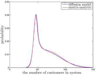
(a) $\rho=1.141$ and $n=50$

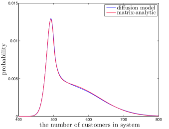
(b) $\rho=1.045$ and $n=500$

Figure 1: The stationary distribution of the customer number in the $M/H_{2}/n+M$ queue.

	Model (4.14)	Matrix-analytic
Mean queue length	$17.27$	$17.16$
Abandonment fraction	$0.1512$	$0.1503$
$\mathbb{P}[N(\infty)>45]$	$0.8675$	$0.8523$
$\mathbb{P}[N(\infty)>50]$	$0.6785$	$0.6726$
$\mathbb{P}[N(\infty)>100]$	$0.08700$	$0.07436$
$\mathbb{P}[N(\infty)>130]$	$0.008662$	$0.003299$

(a) $\rho=1.141$ and $n=50$

	Model (4.14)	Matrix-analytic
Mean queue length	$54.17$	$54.05$
Abandonment fraction	$0.05181$	$0.05173$
$\mathbb{P}[N(\infty)>470]$	$0.9701$	$0.9694$
$\mathbb{P}[N(\infty)>500]$	$0.6838$	$0.6818$
$\mathbb{P}[N(\infty)>600]$	$0.2244$	$0.2229$
$\mathbb{P}[N(\infty)>750]$	$0.008233$	$0.006395$

(b) $\rho=1.045$ and $n=500$

Table 1: Performance measures of the $M/H_{2}/n+M$ queue.

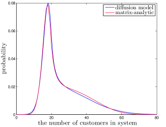
Figure 2: The stationary distribution of the customer number in the $M/H_{2}/n+M$ queue, with $\rho=1.112$ and $n=20$.

Consider an $M/H_{2}/n+M$ queue that has an exponential patience time distribution. We are interested in such a queue because its customer-count process $N=\{N(t):t\geq 0\}$ is a quasi-birth-death process, where $N(t)$ is the number of customers in system at time $t$. The stationary distribution of that can be computed by the matrix-analytic method.

In this example, we take $\alpha=0.5$ for the rate of the exponential patience time distribution and

$$p=(0.9351,0.0649)^{\prime}\qquad\text{and}\qquad\nu=(9.354,0.072)^{\prime}$$

for the hyperexponential service time distribution. The mean service time of the second-type customers is more than one hundred times longer than that of the first type. Although over ninety percent of customers are of the first type, the fraction of its workload is merely ten percent, i.e., $\gamma=(0.1,0.9)^{\prime}$. Such a distribution has a large squared coefficient of variation $c_{s}^{2}=24$.

The queue is approximated by the two-dimensional piecewise OU process $X$ in (4.14). Because the service time distribution is hyperexponential, $P$ is a zero matrix and thus $R=\operatorname{diag}(\nu)$. By (4.15) and (4.16), the drift coefficient of $X$ is

$$b(x)=\begin{pmatrix}-p_{1}\mu\beta-\nu_{1}(x_{1}-p_{1}(x_{1}+x_{2})^{+})-p_{1}\alpha(x_{1}+x_{2})^{+}\\ -p_{2}\mu\beta-\nu_{2}(x_{2}-p_{2}(x_{1}+x_{2})^{+})-p_{2}\alpha(x_{1}+x_{2})^{+}\end{pmatrix}$$ (6.2)

and the covariance matrix of the diffusion coefficient is

$$\Sigma(x)=\begin{pmatrix}p_{1}\mu(\rho+(\rho\wedge 1))&0\\ 0&p_{2}\mu(\rho+(\rho\wedge 1))\end{pmatrix}$$ (6.3)

for all $x\in\mathbb{R}^{2}$.

Three scenarios are considered in this example, in all of which the queue is overloaded. In the first two scenarios, there are $n=50$ and $500$ servers, respectively. The arrival rates are $\lambda=57.071$ and $522.36$, or equivalently, $\rho=1.141$ and $1.045$. By (4.1), $\beta=-1$ in both scenarios. The third scenario, with $n=20$ servers, will be presented shortly.

To compute the stationary distribution of $X$, we use a product reference density given by (5.6) and (5.8). To generate basis functions by the finite element method, we set the truncation rectangle $K=[-7,32]\times[-7,32]$, which is obtained by (5.15) with $\varepsilon_{0}=10^{-7}$, and use a lattice mesh in which all finite elements are $0.5\times 0.5$ squares.

Once the stationary density of $X$ is obtained, one can approximately produce the distribution of $N(\infty)$, the stationary number of customers in system. Note that the probability density of $X_{1}(\infty)+X_{2}(\infty)$ is given by

$$g_{N}(z)=\int_{-\infty}^{+\infty}g(x_{1},z-x_{1})\,\mathrm{d}x_{1}\qquad\text{for }z\in\mathbb{R}\text{.}$$

The distribution of $N(\infty)$ can be approximated by

$$\mathbb{P}[N(\infty)=i]\approx\frac{1}{\sqrt{n}}g_{N}\Big{(}\frac{i-n}{\sqrt{n}}\Big{)}\qquad\text{for }i=0,1,\ldots$$

For the first two scenarios, the distributions of $N(\infty)$ obtained by the diffusion model are illustrated in Figure 1. In the same figure, the stationary distributions computed by the matrix-analytic method are plotted, too. We see good agreement in Figure 1. Comparing the two scenarios, we also find out that the diffusion model in (4.14) is more accurate when the number of servers $n$ is larger. This observation is consistent with the many-server limit theorem for $G/Ph/n+GI$ queues in Dai, He and Tezcan (2010).

The matrix-analytic method can be used because in this queue, the three-dimensional process $\{(Q(t),Z_{1}(t),Z_{2}(t)):t\geq 0\}$ forms a continuous-time Markov chain and the customer-count process $N$ is a quasi-birth-death process. Clearly, $N(t)=Q(t)+Z_{1}(t)+Z_{2}(t)$. At time $t$, $N$ is said to be at level $\ell$ if $N(t)=\ell$. In this example, level $\ell$ consists of $\ell+1$ states if $\ell\leq n$ and it contains $n+1$ states if $\ell>n$. In the matrix-analytic method, the transition rate matrices between adjacent levels are exploited to compute the stationary distribution of $N$ iteratively. Each iteration requires $O(n^{3})$ arithmetic operations. For this queue, the transition rate matrices at different levels are different because the abandonment rate depends on the queue length. For implementation purposes, we assume in the algorithm that at level $\ell>\ell_{0}$ for some $\ell_{0}\gg n$, the abandonment rate at level $\ell$ is $\alpha(\ell_{0}-n)$ rather than $\alpha(\ell-n)$. In other words, the transition rate matrices at level $\ell$ are invariant with respect to $\ell$ when $\ell>\ell_{0}$. We take $\ell_{0}=n+2000$ in all numerical examples. The extra error caused by this modification is negligible, because in this queue, the queue length is in the order of $O(n^{1/2})$ and the chance of the customer number exceeding $\ell_{0}$ is extremely rare.

To investigate the diffusion model in (4.14) quantitatively, we list some steady-state performance measures in Table 1. They include the mean queue length, the fraction of abandoned customers, and the probabilities that the number of customers exceeds certain levels. Using the diffusion model,

$$\text{the mean queue length}\approx\sqrt{n}\int_{\mathbb{R}^{2}}(x_{1}+x_{2})^{+}g(x)\,\mathrm{d}x$$

and

$$\text{the mean number of idle servers}\approx\sqrt{n}\int_{\mathbb{R}^{2}}(x_{1}+x_{2})^{-}g(x)\,\mathrm{d}x.$$

It follows from the latter approximation that

$$\text{the abandonment fraction}\approx 1-\frac{\mu}{\lambda}\Big{(}n-\sqrt{n}\int_{\mathbb{R}^{2}}(x_{1}+x_{2})^{-}g(x)\,\mathrm{d}x\Big{)}.$$

In the table, the tail probability $\mathbb{P}[N(\infty)>\ell]$ is approximated by

$$\mathbb{P}[N(\infty)>\ell]\approx\mathbb{P}\Big{[}X_{1}(\infty)+X_{2}(\infty)>\frac{1}{\sqrt{n}}(\ell-n)\Big{]}\qquad\text{for }\ell=0,1,\ldots$$

and $\mathbb{P}[X_{1}(\infty)+X_{2}(\infty)>(\ell-n)/\sqrt{n}]$ is computed via (6.1). In both scenarios, the diffusion model produces satisfactory numerical estimates.

The computational complexity of the proposed algorithm, whether in computation time or in memory space, does not change with the number of servers $n$. In contrast, the matrix-analytic method becomes computationally expensive when $n$ is large. In particular, the memory usage becomes a serious constraint when a huge number of iterations are required. For the $n=500$ scenario in this example, it took around one hour to finish the matrix-analytic computation and the peak memory usage is nearly five gigabytes. Using the diffusion model and the proposed algorithm, it took less than one minute and the peak memory usage is less than two hundred megabytes on the same computer. See Section 7.4 for more discussion on the computational complexity.

Although the diffusion model is motivated and derived from the theory of many-server queues, it is still relevant for a queue with a modest number of servers. In the third scenario, there are $n=20$ servers and the arrival rate is $\lambda=22.24$. Thus, $\rho=1.112$ and $\beta=-0.5$. In the proposed algorithm, we keep the same truncation rectangle and lattice mesh as in the previous two scenarios, and the reference density is again from (5.6) and (5.8). As illustrated in Figure 2, the diffusion model can still capture the exact stationary distribution for a queue with as few as twenty servers.

6.2 Example 2: an $M/H_{2}/n$ queue

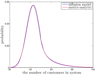
(a) $\rho=0.8586$ and $n=50$

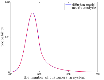
(b) $\rho=0.9553$ and $n=500$

Figure 3: The stationary distribution of the customer number in the $M/H_{2}/n$ queue.

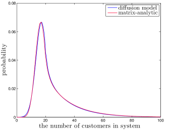
Figure 4: The stationary distribution of the customer number in the $M/H_{2}/n$ queue, with $\rho=0.8882$ and $n=20$.

	Model (4.14)	Matrix-analytic
Mean queue length	$2.267$	$2.419$
$\mathbb{P}[N(\infty)>40]$	$0.6908$	$0.6578$
$\mathbb{P}[N(\infty)>50]$	$0.2072$	$0.2012$
$\mathbb{P}[N(\infty)>70]$	$0.03395$	$0.03655$
$\mathbb{P}[N(\infty)>100]$	$0.003537$	$0.003494$

(a) $\rho=0.8586$ and $n=50$

	Model (4.14)	Matrix-analytic
Mean queue length	$8.753$	$8.800$
$\mathbb{P}[N(\infty)>450]$	$0.9038$	$0.9005$
$\mathbb{P}[N(\infty)>500]$	$0.2285$	$0.2263$
$\mathbb{P}[N(\infty)>600]$	$0.01910$	$0.01908$
$\mathbb{P}[N(\infty)>700]$	$0.002241$	$0.001903$

(b) $\rho=0.9553$ and $n=500$

Table 2: Performance measures of the $M/H_{2}/n$ queue.

In this example, an $M/H_{2}/n$ queue without abandonment is considered. The hyperexponential service time distribution has

$$p=(0.5915,0.4085)^{\prime}\qquad\text{and}\qquad\nu=(5.917,0.454)^{\prime}\text{.}$$

Thus, $c_{s}^{2}=3$ and $\gamma=(0.1,0.9)^{\prime}$. Since there is no abandonment, we must take $\rho<1$ in order for the system to reach a steady state.

The diffusion model in (4.14) with $\alpha=0$ is used. The drift and the diffusion coefficients of $X$ are given by (6.2) and (6.3). The first scenario has $n=50$ servers and the second scenario has $n=500$ servers. The respective arrival rates are $\lambda=42.929$ and $477.64$. Hence, $\rho=0.8586$ and $0.9553$, both yielding $\beta=1$. The product reference density is given by (5.6) and (5.7). With $\varepsilon_{0}=10^{-7}$, the truncation rectangle is set by (5.15) to be $K=[-7,35]\times[-7,35]$, which is divided into $0.5\times 0.5$ finite elements.

The stationary distribution of the number of customers in system is shown in Figure 3. In both scenarios, the diffusion model produces a good approximation of the result by the matrix-analytic method. As in the previous example, the diffusion model is more accurate when the system scale is larger. Several performance measures in steady state are listed in Table 2. As in Table 1, satisfactory agreement can be found between the two approaches.

The third scenario has $n=20$ servers with arrival rate $\lambda=17.76$. Then, $\rho=0.8882$ and $\beta=0.5$. With $\varepsilon_{0}=10^{-7}$, the truncation rectangle is taken to be $K=[-7,79]\times[-7,79]$. The lattice mesh consists of $0.5\times 0.5$ finite elements. The distribution of $N(\infty)$ is shown in Figure 4. For a queue without abandonment, the diffusion model is still useful when the number of servers is modest.

6.3 Example 3: an $M/H_{2}/n+E_{k}$ queue

	$+E_{2}$		$+E_{3}$
	Model (4.20)	Simulation	Model (4.20)	Simulation
Mean queue length	$0.9820$	$1.061$	$1.201$	$1.302$
Abandonment fraction	$0.007974$	$0.008592$	$0.005629$	$0.006115$
$\mathbb{P}[N(\infty)>35]$	$0.8881$	$0.8745$	$0.8896$	$0.8762$
$\mathbb{P}[N(\infty)>40]$	$0.6755$	$0.6399$	$0.6798$	$0.6448$
$\mathbb{P}[N(\infty)>50]$	$0.1671$	$0.1581$	$0.1788$	$0.1707$
$\mathbb{P}[N(\infty)>60]$	$0.03238$	$0.03353$	$0.04420$	$0.04584$

(a) $\rho=0.8586$ and $n=50$

	$+E_{2}$		$+E_{3}$
	Model (4.20)	Simulation	Model (4.20)	Simulation
Mean queue length	$4.960$	$5.048$	$6.455$	$6.569$
Abandonment fraction	$0.001689$	$0.001729$	$0.0007611$	$0.0007931$
$\mathbb{P}[N(\infty)>450]$	$0.9003$	$0.8964$	$0.9022$	$0.8984$
$\mathbb{P}[N(\infty)>480]$	$0.4759$	$0.4643$	$0.4859$	$0.4746$
$\mathbb{P}[N(\infty)>500]$	$0.1995$	$0.1966$	$0.2151$	$0.2124$
$\mathbb{P}[N(\infty)>550]$	$0.02798$	$0.02841$	$0.04412$	$0.04458$

(b) $\rho=0.9553$ and $n=500$

Table 3: Performance measures of the $M/H_{2}/n+E_{k}$ queue with $\rho<1$.

	$+E_{2}$		$+E_{3}$
	Model (4.20)	Simulation	Model (4.20)	Simulation
Mean queue length	$15.03$	$14.94$	$19.44$	$19.31$
Abandonment fraction	$0.1332$	$0.1334$	$0.1303$	$0.1305$
$\mathbb{P}[N(\infty)>45]$	$0.9568$	$0.9490$	$0.9704$	$0.9645$
$\mathbb{P}[N(\infty)>50]$	$0.8780$	$0.8648$	$0.9169$	$0.9066$
$\mathbb{P}[N(\infty)>70]$	$0.3325$	$0.3121$	$0.5037$	$0.4761$
$\mathbb{P}[N(\infty)>90]$	$0.008153$	$0.009354$	$0.03033$	$0.03422$

(a) $\rho=1.141$ and $n=50$

	$+E_{2}$		$+E_{3}$
	Model (4.20)	Simulation	Model (4.20)	Simulation
Mean queue length	$76.50$	$76.20$	$119.5$	$119.1$
Abandonment fraction	$0.04438$	$0.04437$	$0.04340$	$0.04337$
$\mathbb{P}[N(\infty)>480]$	$0.9857$	$0.9846$	$0.9946$	$0.9940$
$\mathbb{P}[N(\infty)>500]$	$0.9390$	$0.9363$	$0.9770$	$0.9756$
$\mathbb{P}[N(\infty)>600]$	$0.3115$	$0.3051$	$0.6733$	$0.6645$
$\mathbb{P}[N(\infty)>700]$	$0.0009757$	$0.0009658$	$0.04260$	$0.04358$

(b) $\rho=1.045$ and $n=500$

Table 4: Performance measures of the $M/H_{2}/n+E_{k}$ queue with $\rho>1$.

Consider an $M/H_{2}/n+E_{k}$ queue, where $k>1$ is a positive integer and $+E_{k}$ signifies an Erlang-$k$ patience time distribution. In this queue, each patience time is the sum of $k$ stages and the stages are iid having an exponential distribution with mean $1/\theta$. When $k>1$, the probability density at zero of an Erlang-$k$ distribution is zero. The diffusion model in (4.14) does not have a stationary distribution when the queue is overloaded. Hence, we evaluate the diffusion model in (4.20) that exploits the patience time hazard rate scaling. In the following numerical experiments, we take $k=2$ or $3$ for the Erlang-$k$ distribution and set $\theta=k$, so the mean patience time is one unit time. The hyperexponential service time distribution is taken to be identical to that in Section 6.2.

The hazard rate function of the Erlang-$k$ distribution is

$$h(t)=\frac{\theta^{k}t^{k-1}}{(k-1)!\sum\limits_{\ell=0}^{k-1}\dfrac{\theta^{\ell}t^{\ell}}{\ell!}}\qquad\text{for }t\geq 0\text{.}$$

For the diffusion model (4.20), it follows from (4.21) that the drift coefficient of $X$ is

$$b(x)=\begin{pmatrix}-p_{1}\mu\beta-\nu_{1}(x_{1}-p_{1}(x_{1}+x_{2})^{+})-p_{1}\eta((x_{1}+x_{2})^{+})\\ -p_{2}\mu\beta-\nu_{2}(x_{2}-p_{2}(x_{1}+x_{2})^{+})-p_{2}\eta((x_{1}+x_{2})^{+})\end{pmatrix}$$ (6.4)

where

$$\eta(z)=\int_{0}^{z}h\Big{(}\frac{\sqrt{n}u}{\lambda}\Big{)}\,\mathrm{d}u=\theta z-\frac{\lambda}{\sqrt{n}}\log\bigg{(}\sum_{m=0}^{k-1}\frac{n^{m/2}\theta^{m}z^{m}}{m!\lambda^{m}}\bigg{)}\qquad\text{for }z\geq 0\text{.}$$

The first two scenarios has $n=50$ and $500$ servers, respectively. Their respective arrival rates are $\lambda=42.929$ and $477.64$. Hence, $\rho=0.8586$ and $0.9553$, both leading to $\beta=1$. In the proposed algorithm, the reference density is chosen according to (5.6) and (5.7). The truncation rectangle is taken to be $K=[-7,35]\times[-7,35]$ and is divided into $0.5\times 0.5$ finite elements. Some performance estimates can be found in Table 3.

The third and fourth scenarios are for the case $\rho>1$. They have $n=50$ and $500$ servers, and arrival rates $\lambda=57.071$ and $522.36$, respectively. Then, $\rho=1.141$ and $1.045$, both having $\beta=-1$. For these two scenarios, we adopt the reference density in (5.6) and (5.14). When $k=2$, each patience time has two stages. The hazard rate function of the patience time distribution has $h(0)=0$ and $h^{(1)}(0)=\theta^{2}$, so $\ell_{0}=1$ in (5.12) and (5.13). Because $\alpha$ in (5.13) depends on $n$, both the reference density and the truncation rectangle change with $n$. With $\varepsilon_{0}=10^{-7}$, the truncation rectangle is set to be $K=[-7,13]\times[-7,13]$ for $n=50$ and to be $K=[-7,16]\times[-7,16]$ for $n=500$. When $k=3$, a patience time consists of three stages. In this case, $h(0)=h^{(1)}(0)=0$ and $h^{(2)}(0)=8\theta^{3}$, so $\ell_{0}=2$. We set $K=[-7,11]\times[-7,11]$ for $n=50$ and $K=[-7,15]\times[-7,15]$ for $n=500$. All truncation rectangles are partitioned into $0.5\times 0.5$ finite elements. The performance estimates are listed in Table 4.

To evaluate the diffusion model (4.20), we list corresponding simulation estimates of the performance measures in both tables. As in the previous examples, the diffusion model produces adequate performance approximations.

Theoretically, the matrix-analytic method can be used in this example as the customer-count process $N$ is also a quasi-birth-death process. But it is impractical because the computational complexity is too high. Consider the case $k=2$. Let $V_{1}(t)$ and $V_{2}(t)$ be the respective numbers of waiting customers whose patience times are in the first and in the second stage at time $t$. For this $M/H_{2}/n+E_{2}$ queue, the four-dimensional process $\{(V_{1}(t),V_{2}(t),Z_{1}(t),Z_{2}(t)):t\geq 0\}$ is a continuous-time Markov chain. At level $\ell$, there are $\ell+1$ states if $\ell\leq n$ and there are $(n+1)(\ell-n+1)$ states if $\ell>n$. The number of states at level $\ell$ is formidable when $\ell$ is large. Even if we may truncate the state space using the technique described in Section 6.1, the number of states is still too large to apply the matrix-analytic method. In fact, we are not aware of any other numerical methods other than simulation that can produce approximations in Tables 3 and 4.

6.4 Example 4: an $M/H_{2}/n+H_{2}$ queue

	Model (4.14)	Model (4.20)	Simulation
Mean queue length	$0.4709$	$4.869$	$4.845$
Abandonment fraction	$0.1714$	$0.1504$	$0.1499$
$\mathbb{P}[N(\infty)>40]$	$0.9578$	$0.9749$	$0.9728$
$\mathbb{P}[N(\infty)>50]$	$0.3158$	$0.6377$	$0.6111$
$\mathbb{P}[N(\infty)>60]$	$1.044\times 10^{-7}$	$0.1895$	$0.1737$
$\mathbb{P}[N(\infty)>70]$	$1.097\times 10^{-11}$	$0.02568$	$0.02142$

(a) $\rho=1.141$ and $n=50$

	Model (4.14)	Model (4.20)	Simulation
Mean queue length	$1.475$	$6.359$	$6.413$
Abandonment fraction	$0.05863$	$0.05517$	$0.05512$
$\mathbb{P}[N(\infty)>480]$	$0.8663$	$0.8929$	$0.8881$
$\mathbb{P}[N(\infty)>500]$	$0.3192$	$0.4822$	$0.4720$
$\mathbb{P}[N(\infty)>520]$	$9.274\times 10^{-5}$	$0.1074$	$0.1050$
$\mathbb{P}[N(\infty)>550]$	$-4.488\times 10^{-9}$	$0.006616$	$0.006248$

(b) $\rho=1.045$ and $n=500$

Table 5: Performance measures of the $M/H_{2}/n+H_{2}$ queue.

Let us consider an example in which the patience time hazard rate function changes rapidly near the origin. As pointed out by Reed and Tezcan (2009), the performance of such a queue is sensitive to the patience time distribution in a neighborhood of zero. A model that exploits the patience time density at zero solely may not produce adequate performance estimates. In this example, the patience times follow a two-phase hyperexponential distribution that has

$$\hat{p}=(0.9,0.1)^{\prime}\qquad\text{and}\qquad\hat{\nu}=(1,200)^{\prime}\text{.}$$

In other words, there are two types of patience times. Ninety percent of patience times are exponentially distributed with mean one and ten percent are exponentially distributed with mean $0.005$. We take the same hyperexponential service time distribution as in Sections 6.2 and 6.3.

The hazard rate function of the hyperexponential patience time distribution is

$$h(t)=\frac{\hat{p}_{1}\hat{\nu}_{1}\exp(-\hat{\nu}_{1}t)+\hat{p}_{2}\hat{\nu}_{2}\exp(-\hat{\nu}_{2}t)}{\hat{p}_{1}\exp(-\hat{\nu}_{1}t)+\hat{p}_{2}\exp(-\hat{\nu}_{2}t)}\qquad\text{for }t\geq 0\text{.}$$

The drift coefficient of $X$ in (4.20) is also given by (6.4) where

$$\eta(z) =\int_{0}^{z}h\Big{(}\frac{\sqrt{n}u}{\lambda}\Big{)}\,\mathrm{d}u$$

$$=-\frac{\lambda}{\sqrt{n}}\log\Big{(}\hat{p}_{1}\exp\Big{(}-\frac{\sqrt{n}}{\lambda}\hat{\nu}_{1}z\Big{)}+\hat{p}_{2}\exp\Big{(}-\frac{\sqrt{n}}{\lambda}\hat{\nu}_{2}z\Big{)}\Big{)}\qquad\text{for }z\geq 0\text{.}$$

In this example, we have

$$h(0)=\hat{p}_{1}\hat{\nu}_{1}+\hat{p}_{2}\hat{\nu}_{2}=20.9\qquad\text{and\qquad}h^{(1)}(0)=-\hat{p}_{1}\hat{p}_{2}(\hat{\nu}_{1}-\hat{\nu}_{2})^{2}=-3564.1.$$

Thus, $\ell_{0}=0$ and the hazard rate function has a steep slope near the origin. Since the zeroth degree Taylor’s approximation in (5.9) may bring on too much error, the reference density exploiting the lowest-order nonzero derivative at the origin could be erroneous.

To choose an appropriate reference density, an auxiliary queue is used again. As in Section 5.3, the auxiliary queue is an $M/H_{2}/n+M$ queue that shares the same arrivals and service times with the $M/H_{2}/n+H_{2}$ queue. Let $\alpha>0$ be the rate of the exponential patience time distribution. We take $\alpha=\hat{\nu}_{1}\wedge\hat{\nu}_{2}$ so that the patience times in the auxiliary queue are all of the type with the longer mean. If the queue lengths are equal, the abandonment rate in the auxiliary queue must be lower than that in the original queue. Therefore, the queue length decays slower in the former queue and the reference density for model (4.14) of the auxiliary queue should work. This observation leads to a reference density that follows (5.6) and (5.14), but in this example, we take $\alpha=\hat{\nu}_{1}\wedge\hat{\nu}_{2}$ and solve (5.11) to find $q_{0}$.

Two scenarios with $n=50$ and $500$ servers are investigated. The respective arrival rates are $\lambda=57.071$ and $522.36$. Thus, $\rho=1.141$ and $1.045$ and both scenarios have $\beta=-1$. By solving (5.11), we have $q_{0}=0.165$ for the first scenario and $q_{0}=0.0059$ for the second scenario. The reference density follows (5.6) and (5.14) with $\alpha=\hat{\nu}_{1}=1$. With $\varepsilon_{0}=10^{-7}$, the truncation rectangle is $K=[-7,9]\times[-7,9]$, partitioned into $0.5\times 0.5$ finite elements. The performance estimates obtained by the diffusion model (4.20) are compared with the simulation results in Table 5. The performance estimates are still quite accurate.

We also put the performance estimates produced by the diffusion model (4.14) in this table. For this model, the reference density follows (5.6) and (5.8) with $\alpha=h(0)=20.9$. In the proposed algorithm, the mesh for model (4.20) is used again. Because in this example, using the patience time density at zero solely cannot capture the behavior of the abandonment process, model (4.14) fails to produce proper performance estimates.

7 Implementation issues

The proposed algorithm was implemented using the C++ programming language. The package was tested on both Linux and Windows platforms. In this section, we discuss several important issues arising from the implementation. They are crucial for using the algorithm to solve practical problems. To demonstrate these issues, the second scenario with $n=500$ servers in Section 6.1 is investigated throughout this section. The diffusion model (4.14) is used to approximate the $M/H_{2}/n+M$ queue.

7.1 Influence of the reference density

(a) $K={[-7,10]\times[-7,10]}$

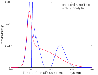
(b) $K={[-7,32]\times[-7,32]}$

Figure 5: The output of the proposed algorithm with the “naive” reference density.

The reference density plays a key role in the algorithm. If the function $r$ does not satisfy (3.1), the sequence of spaces $\{H_{k}:k\in\mathbb{N}\}$ may not converge to $H$ in $L^{2}(\mathbb{R}^{d},r)$ and the output of the algorithm may significantly deviate from the exact stationary density. To demonstrate this issue, let us consider a “naive” reference density.

To produce a “naive” reference density, we consider a queue that has the same arrival process and patience time distribution as the $M/H_{2}/n+M$ queue. This new queue has an exponential service time distribution and its mean service time is equal to that of the $M/H_{2}/n+M$ queue. For this $M/M/n+M$ queue, the diffusion model (4.14) is a one-dimensional piecewise OU process whose stationary density is given by (5.5). The “naive” reference density is a product reference density in (5.6) with each $r_{j}$ being the stationary density in (5.5). In other words, the “naive” reference density is obtained by pretending the service time distribution to be exponential.

Let us apply the “naive” reference density. With $\varepsilon_{0}=10^{-7}$, the truncation rectangle is set to be $K=[-7,10]\times[-7,10]$ and is partitioned into $0.5\times 0.5$ finite elements. As shown in Figure 5a, the output of the proposed algorithm noticeably deviates from the exact stationary distribution. To further confirm that the “naive” reference density cannot work, we next test the truncation rectangle $K=[-7,32]\times[-7,32]$, which is used in Section 6.1 along with the proposed reference density. In this case, the matrix $A$ in (3.12) is close to singular and its condition number is $3.52\times 10^{190}$. Figure 5b manifests the severe error in the algorithm output.

Recall that in this example, the hyperexponential service time distribution has $c_{s}^{2}=24$. Comparing (5.5) with (5.8), we can tell that the decay rate of the “naive” reference density is much larger than that of the proposed reference density. If Conjecture 3 is true, one can expect that the “naive” reference density decays much faster than the stationary density and the second condition in (3.1) may not hold. In this case, the ratio function $q$ is no longer in $L^{2}(\mathbb{R}^{d},r)$ and consequently, the algorithm fails to produce any adequate estimate of the ratio function.

7.2 Mesh selection

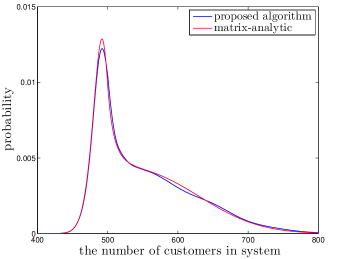
(a) $1.0\times 1.0$ finite elements

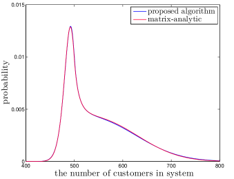
(b) $0.25\times 0.25$ finite elements

Figure 6: The output of the proposed algorithm with different meshes.

	$0.5\times 0.5$	$0.25\times 0.25$	Matrix-analytic
Mean queue length	$54.17$	$54.17$	$54.05$
Abandonment fraction	$0.05181$	$0.05182$	$0.05173$
$\mathbb{P}[N(\infty)>470]$	$0.9701$	$0.9702$	$0.9694$
$\mathbb{P}[N(\infty)>500]$	$0.6838$	$0.6835$	$0.6818$
$\mathbb{P}[N(\infty)>600]$	$0.2244$	$0.2241$	$0.2229$
$\mathbb{P}[N(\infty)>750]$	$0.008233$	$0.008246$	$0.006395$

Table 6: The output of the proposed algorithm using different meshes.

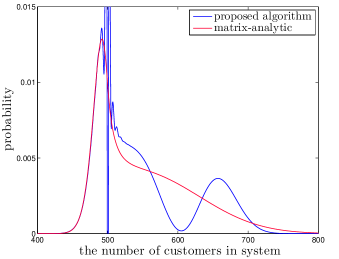
(a) $0.25\times 0.25$ finite elements

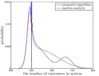
(b) $0.125\times 0.125$ finite elements

Figure 7: The output of the proposed algorithm with the “naive” reference density and different meshes.

When both the reference density and the truncation hypercube are fixed, using a finer mesh may produce smaller approximation error. However, a finer mesh yields more basis functions, which in turn lead to a larger condition number for the matrix $A$ in (3.12). If the condition number of $A$ is too large, the round-off error in solving (3.12) becomes considerable. So a finer mesh does not necessarily yield a more accurate output.

Let us test different meshes for the second scenario in Section 6.1. We keep the same settings for the algorithm except the size of finite elements. The output with $1.0\times 1.0$ finite elements is plotted in Figure 6a. With this mesh, the algorithm does not perform well at the intervals where the stationary density varies quickly. We need a finer mesh to improve the accuracy. In this case, the condition number of $A$ is $5.70\times 10^{20}$. Recall that to produce the curve in Figure 1b, we use a mesh consisting of $0.5\times 0.5$ finite elements. With this mesh, the condition number of $A$ is $1.15\times 10^{23}$. When the element size is further reduced to $0.25\times 0.25$, the condition number of $A$ grows to $7.13\times 10^{27}$. As illustrated in Figure 6b, the output of the algorithm fits the exact stationary distribution well. When we compare Figures 1b and 6b, however, there is barely any difference noticeable between the algorithm outputs. To confirm that this mesh is not superior to the one with $0.5\times 0.5$ finite elements, we list several performance estimates in Table 6. In this table, the results in Table 1b are duplicated for comparison purposes. The difference between the algorithm outputs using these two meshes is negligible. Considering the modeling error of the diffusion model, we can assert that using $0.5\times 0.5$ finite elements is sufficient to produce an accurate approximation for this queue.

Given an appropriate reference density and the associated truncation hypercube, the above discussion has demonstrated an approach to selecting a mesh. Beginning with two meshes, with one finer than the other, we compare the algorithm outputs using these two meshes. If obvious difference is observed, the coarser mesh should be discarded and a further finer mesh is explored. Continue this procedure until the difference between the outputs of two meshes are negligible. Then, the coarser one of the remaining two is selected as an appropriate mesh.

We would also demonstrate that with an improper reference density, a finer mesh cannot make the algorithm yield an adequate output. Let us go back to the example in Section 7.1 with the “naive” reference density. We set the truncation rectangle to be $K=[-7,32]\times[-7,32]$ and the size of finite elements to be $0.25\times 0.25$. The output is shown in Figure 7a. Although the curve appears smoother than the one in Figure 5b with $0.5\times 0.5$ finite elements, the output still fails to capture the exact stationary distribution. This time, the condition number of $A$ is $3.91\times 10^{195}$. There is no doubt that such an ill-conditioned matrix will bring about a huge round-off error in solving (3.12). A mesh with $0.125\times 0.125$ finite elements is also investigated and the algorithm output is plotted in Figure 7b. The condition number of $A$ increases to $6.35\times 10^{198}$ and the algorithm misses the target as well.

7.3 Gauss-Legendre quadrature

	$m=4$	$m=8$	$m=16$	Matrix-analytic
Mean queue length	$54.17$	$54.17$	$54.17$	$54.05$
Abandonment fraction	$0.05181$	$0.05181$	$0.05181$	$0.05173$
$\mathbb{P}[N(\infty)>470]$	$0.9701$	$0.9701$	$0.9701$	$0.9694$
$\mathbb{P}[N(\infty)>500]$	$0.6833$	$0.6838$	$0.6839$	$0.6818$
$\mathbb{P}[N(\infty)>600]$	$0.2245$	$0.2244$	$0.2244$	$0.2229$
$\mathbb{P}[N(\infty)>750]$	$0.008235$	$0.008233$	$0.008232$	$0.006395$

Table 7: The output of the proposed algorithm with different quadrature orders.

Before solving the linear system (3.12), we must generate the matrix $A$ and the vector $v$ whose entries are given by (3.13). We follow a Gauss-Legendre quadrature rule to compute the integral for each entry. The integral is taken over a two-dimensional rectangle and the quadrature rule evaluates the integrand at $m$ points in each dimension. The results are more accurate when a larger $m$ is used. In Section 6, we take $m=8$ in the numerical examples. Here, we briefly discuss the impact of the order $m$.

Several performance estimates are listed in Table 7. We keep the same settings for the algorithm except the quadrature order in each dimension. For the convenience of comparison, the results in Table 1b are duplicated in this table. Clearly, the Gauss-Legendre quadrature of order $m\geq 4$ is sufficiently accurate for our purposes.

7.4 Computational complexity

	$1.0\times 1.0$	$0.5\times 0.5$	$0.25\times 0.25$	$0.125\times 0.125$
Dimension $m_{C}$	$5776$	$23716$	$96100$	$386884$
Constructing $A$ and $v$	$6.63$	$27.3$	$109$	$455$
Solving (3.12)	$0.0780$	$0.359$	$2.29$	$18.2$

Table 8: Computation time (in seconds) of the proposed algorithm using different meshes.

Let $d$, the dimension of the diffusion model, be fixed. The size of $A$ is $m_{C}\times m_{C}$ where $m_{C}$ is the dimension of the functional space $C$ given by (3.18). The matrix $A$ is sparse. There are at most $6^{d}$ nonzero entries in each row or column. Hence, it takes $O(m_{C})$ arithmetic operations to construct $A$. We may apply Gaussian elimination to solve the linear system (3.12). When the basis functions are properly ordered, the nonzero entries of $A$ are confined to a diagonally bordered band of width $O(m_{C}^{(d-1)/d})$. Hence, solving (3.12) requires $O(m_{C}^{(2d-1)/d})$ operations as $m_{C}\rightarrow\infty$.

The computation time (measured by seconds) for various meshes can be found in Table 8, where we list both the time for constructing $A$ and $v$ and the time for solving (3.12). When computing $A$ and $v$, we follow a Gauss-Legendre quadrature rule with $m=8$ points in each dimension. The truncation rectangle is set to be $K=[-7,32]\times[-7,32]$. Each mesh is obtained by setting the size of finite elements. The dimension $m_{C}$ increases by around four times as the width of each finite element is reduced by half. The proposed algorithm is tested on a laptop with a 2.66GHz Intel Core 2 Duo processor and eight gigabytes memory. Both $A$ and $v$ are produced by our C++ package. The linear system (3.12) is solved by Matlab. These two parts are connected via a MEX interface that comes with Matlab.

8 Concluding remarks

In this paper, we proposed two approximate models for many-server queues with customer abandonment. Both these models are diffusion processes and they differ in how the abandonment process is approximated. A finite element algorithm was proposed for computing the stationary distribution of each model. The essential part of the algorithm is a reference density that controls the convergence of the algorithm. To construct a reference density, we conjectured that the limit queue length process has a certain Gaussian tail. Using this conjecture, we proposed a systematic approach to choosing a reference density. With the proposed reference density, the output of the algorithm is stable and accurate. Numerical examples indicate that the diffusion models are good approximations for many-server queues.

Assume that the stationary density $g$ is twice differentiable in $\mathbb{R}^{d}$ and vanishes at infinity. Using the basic adjoint relationship (2.7) and applying integration by parts twice, we have

$$\mathcal{G}^{\ast}g(x)=0\qquad\text{for all }x\in\mathbb{R}^{d}$$

where $\mathcal{G}^{\ast}$ is the adjoint operator of the generator $\mathcal{G}$. Fix a finite domain $K\subset\mathbb{R}^{d}$ large enough. One can solve the stationary density $g$ by the Dirichlet problem

$$\begin{cases}\mathcal{G}^{\ast}g(x)=0&\text{for }x\text{ in the interior of }K\text{,}\\ g(x)=0&\text{for }x\text{ on the boundary of }K\text{.}\end{cases}$$

Such a Dirichlet problem can be solved via a finite difference algorithm. Alternatively, for each test function $f$, one may apply integration by parts once to the basic adjoint relationship to obtain an equation that involves the first derivatives of $g$ and the first derivatives of $f$. From this weak formulation, fixing a large enough finite domain $K$ and assuming that $g$ is zero on the boundary of $K$, one may apply a standard Galerkin finite element method to compute the stationary density $g$ on $K$. See, e.g., Kovalov, Linetsky and Marcozzi (2007). Both the finite difference algorithm and the Galerkin method do not use a reference density. A future research topic is to compare the efficiency and accuracy of these two algorithms with the proposed algorithm in this paper.

The dimension of the functional space $C$ in Section 3.3 grows exponentially in $d$, the dimension of the diffusion model. As a consequence, both the computation time and the memory usage increases exponentially in $d$. When $d$ is not small, the curse of dimensionality is a serious challenge for the proposed algorithm as well as any other algorithms. To reduce the dimension of $C$, one possible approach is to investigate a reference density that potentially shares more common features with the stationary density. Such a reference density may enable us to compute the stationary density with a moderate number of basis functions when $d$ is not small. Another possible direction to reduce the computational complexity of the algorithm is to investigate a low-rank matrix approximation for the linear system (3.12). The technique of random sampling may be explored. See Kannan and Vempala (2010) for more details.

Appendix

Proof of Proposition 2

Recall that $K$ is the compact support of $C$ and the basis functions of $C$ are given by (3.17). We use $C_{0}^{1}(K)$ to denote the set of real-valued functions on a neighborhood of $K$ that are continuously differentiable and have compact support in $K$. Clearly, $C\subset C_{0}^{1}(K)$. For any $f,\hat{f}\in C_{0}^{1}(K)$, we define an inner product by

$$\langle f,\hat{f}\rangle_{D(K)}=\sum_{j=1}^{d}\int_{K}\frac{\partial f(x)}{\partial x_{j}}\frac{\partial\hat{f}(x)}{\partial x_{j}}\,\mathrm{d}x$$

and let $W_{0}^{1,2}(K)$ be the closure of $C_{0}^{1}(K)$ in the norm induced by this inner product. Then, $W_{0}^{1,2}(K)$ is a Hilbert space and $C\subset W_{0}^{1,2}(K)$.

Proof of Proposition 2.

Since $\mathcal{G}$ is a linear operator, it suffices to show that for any $f_{0}\in C$, we must have $f_{0}=0$ if $\mathcal{G}f_{0}=0$ in $L^{2}(\mathbb{R}^{d},r)$. The uniform elliptic operator $\mathcal{G}$ can be written into the divergence form as in (8.1) of Gilbarg and Trudinger (2001), i.e.,

$$\mathcal{G}f(x)=\sum_{j=1}^{d}\hat{b}_{j}(x)\frac{\partial f(x)}{\partial x_{j}}+\frac{1}{2}\sum_{j=1}^{d}\sum_{\ell=1}^{d}\frac{\partial(\Sigma_{j\ell}(x)\partial f(x)/\partial x_{j})}{\partial x_{\ell}}$$

for each $f\in C_{b}^{2}(\mathbb{R}^{d})$, where

$$\hat{b}_{j}(x)=b_{j}(x)-\frac{1}{2}\sum_{\ell=1}^{d}\frac{\partial\Sigma_{j\ell}(x)}{\partial x_{\ell}}.$$

Let $U\subset\mathbb{R}^{d}$ be a connected open set that is bounded and contains $K$. Since $r>0$ and $\mathcal{G}f_{0}$ is continuous in the interior of each finite element, we must have $\mathcal{G}f_{0}=0$ in $K$ except on the boundaries of certain finite elements where $\mathcal{G}f_{0}$ is not defined. Hence, $\mathcal{G}f_{0}=0$ in $U$ in the weak sense (see (8.2) of Gilbarg and Trudinger (2001)). Note that $b$, $\Sigma$, and the partial derivatives of $\Sigma$ are all continuous, so both $\hat{b}$ and $\Sigma$ are bounded in $U$. Because $f_{0}\in W_{0}^{1,2}(K)$, it follows from Corollary 8.2 of Gilbarg and Trudinger (2001) that $f_{0}=0$ in $K$, and thus $f_{0}=0$ in $\mathbb{R}^{d}$. ∎

Proof of Proposition 3

Given a compact set $K\subset\mathbb{R}^{d}$, let $C_{b}^{2}(K)$ be the set of real-valued functions on a neighborhood of $K$ that are twice continuously differentiable with bounded first and second derivatives in $K$. For each $f\in C_{b}^{2}(K)$, define a norm $\left\|\cdot\right\|_{H^{2}(K)}$ by

$$\left\|f\right\|_{H^{2}(K)}^{2}=\int_{K}\bigg{(}f^{2}(x)+\max_{j=1,\ldots,d}\Big{(}\frac{\partial f(x)}{\partial x_{j}}\Big{)}^{2}+\max_{j,\ell=1,\ldots,d}\Big{(}\frac{\partial^{2}f(x)}{\partial x_{j}\partial x_{\ell}}\Big{)}^{2}\bigg{)}r(x)\,\mathrm{d}x.$$

Because both $b$ and $\Sigma$ are bounded in $K$, there exists $\kappa_{0}(K)>0$ such that

$$\int_{K}(\mathcal{G}f(x))^{2}r(x)\,\mathrm{d}x\leq\kappa_{0}(K)\left\|f\right\|_{H^{2}(K)}^{2}\qquad\text{for all }f\in C_{b}^{2}(K)\text{.}$$ (.1)

Let $\bar{C}_{b}^{2}(K)$ be the closure of $C_{b}^{2}(K)$ in the above norm. A standard procedure can be used to define the first-order and the second-order derivatives for each $f\in\bar{C}_{b}^{2}(K)$. Then, the operator $\mathcal{G}$ can be extended to $\bar{C}_{b}^{2}(K)$ and inequality (.1) holds for all $f\in\bar{C}_{b}^{2}(K)$.

Proof of Proposition 3.

It suffices to prove that for any $f_{0}\in C_{b}^{2}(\mathbb{R}^{d})$, there exists a sequence of functions $\{\varphi_{k}\in C_{k}:k\in\mathbb{N}\}$ such that

$$\left\|\mathcal{G}\varphi_{k}-\mathcal{G}f_{0}\right\|\rightarrow 0\qquad\text{as }k\rightarrow\infty.$$

Fix $\varepsilon>0$. Because $K_{k}\uparrow\mathbb{R}^{d}$ as $k\rightarrow\infty$, by (3.2) and the Cauchy-Schwartz inequality, there exists $a\in\mathbb{N}$ such that

$$\int_{\mathbb{R}^{d}\setminus K_{a}}(\mathcal{G}f_{0}(x))^{2}r(x)\,\mathrm{d}x<\frac{\varepsilon^{2}}{2}.$$ (.2)

Consider the finite hypercube $K_{a}$. By (.1), there exists $\kappa_{0}(K_{a})>0$ such that

$$\int_{K_{a}}(\mathcal{G}f(x))^{2}r(x)\,\mathrm{d}x\leq\kappa_{0}(K_{a})\left\|f\right\|_{H^{2}(K_{a})}^{2}\qquad\text{for all }f\in\bar{C}_{b}^{2}(K_{a})\text{.}$$ (.3)

A polynomial can be used to approximate $f_{0}$ on $K_{a}$. By Proposition 7.1 in the appendix of Ethier and Kurtz (1986), there exists a polynomial $f_{\operatorname*{p}}$ such that

$$\left\|f_{\operatorname*{p}}-f_{0}\right\|_{H^{2}(K_{a})}<\frac{\varepsilon}{2\sqrt{2\kappa_{0}(K_{a})}}.$$

For the lattice mesh $\Delta_{k}$, let $\Lambda_{a,k}$ be the set of its nodes in the interior of $K_{a}$. For any $k\geq a$, let $\varphi_{k}$ be a function in $C_{k}$ such that $\varphi_{k}(x)=0$ for all $x\in\mathbb{R}^{d}\setminus K_{a}$ and

$$\varphi_{k}(x)=f_{\operatorname*{p}}(x)\qquad\text{and}\qquad\frac{\partial\varphi_{k}(x)}{\partial x_{j}}=\frac{\partial f_{\operatorname*{p}}(x)}{\partial x_{j}}$$

for $j=1,\ldots,d$ and all $x\in\Lambda_{a,k}$. Clearly, $\varphi_{k}\in\bar{C}_{b}^{2}(K_{a})$. Because the sequence of meshes $\{\Delta_{k}:k\in\mathbb{N}\}$ is regularly refined, there exists a constant $\kappa_{1}>0$ such that $\eta_{\Delta_{k}}<\kappa_{1}$ for all $k\geq a$. Using the interpolation error estimate in Theorem 6.6 of Oden and Reddy (1976), we have

$$\left\|\varphi_{k}-f_{\operatorname*{p}}\right\|_{H^{2}(K_{a})}\leq\kappa_{1}^{2}\kappa_{2}\kappa_{3}\Big{(}\int_{\mathbb{R}^{d}}r(x)\,\mathrm{d}x\Big{)}^{1/2}\left|\Delta_{k}\right|^{2},$$

where $\kappa_{2}>0$ is a constant independent of $\Delta_{k}$ and $f_{\operatorname*{p}}$, and

$$\kappa_{3}=\sup\left\{\left|\frac{\partial^{4}f_{\operatorname*{p}}(x)}{\partial x_{1}^{m_{1}}\cdots\partial x_{d}^{m_{d}}}\right|:x\in K_{a};\,m_{1}+\cdots+m_{d}=4\right\}<\infty.$$

Hence, there exists $\delta_{0}>0$ such that

$$\left\|\varphi_{k}-f_{\operatorname*{p}}\right\|_{H^{2}(K_{a})}<\frac{\varepsilon}{2\sqrt{2\kappa_{0}(K_{a})}}$$

whenever $\left|\Delta_{k}\right|<\delta_{0}$. In this case,

$$\left\|\varphi_{k}-f_{0}\right\|_{H^{2}(K_{a})}\leq\left\|\varphi_{k}-f_{\operatorname*{p}}\right\|_{H^{2}(K_{a})}+\left\|f_{\operatorname*{p}}-f_{0}\right\|_{H^{2}(K_{a})}<\frac{\varepsilon}{\sqrt{2\kappa_{0}(K_{a})}}.$$

By (.3),

$$\int_{K_{a}}(\mathcal{G}\varphi_{k}(x)-\mathcal{G}f_{0}(x))^{2}r(x)\,\mathrm{d}x\leq\kappa_{0}(K_{a})\left\|\varphi_{k}-f_{0}\right\|_{H^{2}(K_{a})}^{2}<\frac{\varepsilon^{2}}{2}.$$ (.4)

It follows from (.2) and (.4) that $\left\|\mathcal{G}\varphi_{k}-\mathcal{G}f_{0}\right\|<\varepsilon$ whenever $k\geq a$ and $\left|\Delta_{k}\right|<\delta_{0}$. ∎

References

- Brown et al. (2005) {barticle}[author] \bauthor\bsnmBrown, \bfnmL.\binitsL., \bauthor\bsnmMandelbaum, \bfnmA.\binitsA., \bauthor\bsnmSakov, \bfnmA.\binitsA., \bauthor\bsnmZeltyn, \bfnmS.\binitsS., \bauthor\bsnmZhao, \bfnmL.\binitsL. and \bauthor\bsnmShen, \bfnmHaipeng\binitsH. (\byear2005). \btitleStatistical Analysis of a Telephone Call Center: A Queueing-Science Perspective. \bjournalJournal of the American Statistical Association \bvolume100 \bpages36-50. \endbibitem
- Browne and Whitt (1995) {binproceedings}[author] \bauthor\bsnmBrowne, \bfnmSid\binitsS. and \bauthor\bsnmWhitt, \bfnmWard\binitsW. (\byear1995). \btitlePiecewise-Linear Diffusion Processes. In \bbooktitleAdvances in Queueing (\beditor\bfnmJ.\binitsJ. \bsnmDshalalow, ed.) \bpages463–480. \bpublisherCRC Press, \baddressBoca Raton, FL. \endbibitem
- Dai and Dieker (2010) {btechreport}[author] \bauthor\bsnmDai, \bfnmJ. G.\binitsJ. G. and \bauthor\bsnmDieker, \bfnmA. B.\binitsA. B. (\byear2010). \btitleNonnegativity of solutions to the basic adjoint relationship for some diffusion processes \btypeTechnical Report, \binstitutionGeorgia Institute of Technology. \endbibitem
- Dai and Harrison (1991) {barticle}[author] \bauthor\bsnmDai, \bfnmJ. G.\binitsJ. G. and \bauthor\bsnmHarrison, \bfnmJ. Michael\binitsJ. M. (\byear1991). \btitleSteady-state analysis of RBM in a rectangle: numerical methods and a queueing application. \bjournalAnnals of Applied Probability \bvolume1 \bpages16–35. \endbibitem
- Dai and Harrison (1992) {barticle}[author] \bauthor\bsnmDai, \bfnmJ. G.\binitsJ. G. and \bauthor\bsnmHarrison, \bfnmJ. Michael\binitsJ. M. (\byear1992). \btitleReflected Brownian motion in an orthant: numerical methods for steady-state analysis. \bjournalAnnals of Applied Probability \bvolume2 \bpages65–86. \endbibitem
- Dai and He (2010) {barticle}[author] \bauthor\bsnmDai, \bfnmJ. G.\binitsJ. G. and \bauthor\bsnmHe, \bfnmS.\binitsS. (\byear2010). \btitleCustomer abandonment in many-server queues. \bjournalMathematics of Operations Research \bvolume35 \bpages347-362. \endbibitem
- Dai, He and Tezcan (2010) {barticle}[author] \bauthor\bsnmDai, \bfnmJ. G.\binitsJ. G., \bauthor\bsnmHe, \bfnmS.\binitsS. and \bauthor\bsnmTezcan, \bfnmTolga\binitsT. (\byear2010). \btitleMany-server diffusion limits for queues. \bjournalAnnals of Applied Probability \bvolume20 \bpages1854–1890. \endbibitem
- Dieker and Gao (2011) {btechreport}[author] \bauthor\bsnmDieker, \bfnmA. B.\binitsA. B. and \bauthor\bsnmGao, \bfnmX.\binitsX. (\byear2011). \btitlePositive recurrence of piecewise Ornstein-Uhlenbeck processes and common quadratic Lyapunov functions \btypeTechnical Report, \binstitutionGeorgia Institute of Technology. \endbibitem
- Ethier and Kurtz (1986) {bbook}[author] \bauthor\bsnmEthier, \bfnmStewart N.\binitsS. N. and \bauthor\bsnmKurtz, \bfnmThomas G.\binitsT. G. (\byear1986). \btitleMarkov Processes: Characterization and Convergence. \bpublisherWiley, \baddressNew York. \endbibitem
- Gamarnik and Goldberg (2011) {bmisc}[author] \bauthor\bsnmGamarnik, \bfnmD.\binitsD. and \bauthor\bsnmGoldberg, \bfnmD.\binitsD. (\byear2011). \btitleSteady-state queue in the Halfin-Whitt regime. \bnotepreprint. \endbibitem
- Gamarnik and Momčilović (2008) {barticle}[author] \bauthor\bsnmGamarnik, \bfnmDavid\binitsD. and \bauthor\bsnmMomčilović, \bfnmPetar\binitsP. (\byear2008). \btitleSteady-state analysis of a multi-server queue in the Halfin-Whitt regime. \bjournalAdvances in Applied Probability \bvolume40 \bpages548–577. \endbibitem
- Garnett, Mandelbaum and Reiman (2002) {barticle}[author] \bauthor\bsnmGarnett, \bfnmO.\binitsO., \bauthor\bsnmMandelbaum, \bfnmA.\binitsA. and \bauthor\bsnmReiman, \bfnmM.\binitsM. (\byear2002). \btitleDesigning a Call Center with Impatient Customers. \bjournalManufacturing and Service Operations Management \bvolume4 \bpages208-227. \endbibitem
- Gilbarg and Trudinger (2001) {bbook}[author] \bauthor\bsnmGilbarg, \bfnmDavid\binitsD. and \bauthor\bsnmTrudinger, \bfnmNeil S.\binitsN. S. (\byear2001). \btitleElliptic partial differential equations of second order. \bseriesClassics in Mathematics. \bpublisherSpringer-Verlag, \baddressBerlin. \bnoteReprint of the 1998 edition. \bmrnumberMR1814364 (2001k:35004) \endbibitem
- Halfin and Whitt (1981) {barticle}[author] \bauthor\bsnmHalfin, \bfnmS.\binitsS. and \bauthor\bsnmWhitt, \bfnmW.\binitsW. (\byear1981). \btitleHeavy-traffic limits for queues with many exponential servers. \bjournalOperations Research \bvolume29 \bpages567-588. \endbibitem