Competition between Kondo and RKKY correlations in the presence of strong randomness

Abstract

We propose that competition between Kondo and magnetic correlations results in a novel universality class for heavy fermion quantum criticality in the presence of strong randomness. Starting from an Anderson lattice model with disorder, we derive an effective local field theory in the dynamical mean-field theory (DMFT) approximation, where randomness is introduced into both hybridization and Ruderman-Kittel-Kasuya-Yosida (RKKY) interactions. Performing the saddle-point analysis in the U(1) slave-boson representation, we reveal its phase diagram which shows a quantum phase transition from a spin liquid state to a local Fermi liquid phase. In contrast with the clean limit of the Anderson lattice model, the effective hybridization given by holon condensation turns out to vanish, resulting from the zero mean value of the hybridization coupling constant. However, we show that the holon density becomes finite when variance of hybridization is sufficiently larger than that of the RKKY coupling, giving rise to the Kondo effect. On the other hand, when the variance of hybridization becomes smaller than that of the RKKY coupling, the Kondo effect disappears, resulting in a fully symmetric paramagnetic state, adiabatically connected with the spin liquid state of the disordered Heisenberg model. We investigate the quantum critical point beyond the mean-field approximation. Introducing quantum corrections fully self-consistently in the non-crossing approximation, we prove that the local charge susceptibility has exactly the same critical exponent as the local spin susceptibility, suggesting an enhanced symmetry at the local quantum critical point. This leads us to propose novel duality between the Kondo singlet phase and the critical local moment state beyond the Landau-Ginzburg-Wilson paradigm. The Landau-Ginzburg-Wilson forbidden duality serves the mechanism of electron fractionalization in critical impurity dynamics, where such fractionalized excitations are identified with topological excitations.

I Introduction

Interplay between interactions and disorders has been one of the central issues in modern condensed matter physics Interaction_Disorder_Book ; RMP_Disorder_Interaction . In the weakly disordered metal the lowest-order interaction-correction was shown to modify the density of states at the Fermi energy in the diffusive regime AAL , giving rise to non-Fermi liquid physics particulary in low dimensions less than $d=3$ while further enhancement of electron correlations was predicted to cause ferromagnetism Disorder_FM . In an insulating phase spin glass appears ubiquitously, where the average of the spin moment vanishes in the long time scale, but local spin correlations become finite, making the system away from equilibrium SG_Review .

An outstanding question is the role of disorder in the vicinity of quantum phase transitions Disorder_QCP_Review1 ; Disorder_QCP_Review2 , where effective long-range interactions associated with critical fluctuations appear to cause non-Fermi liquid physics Disorder_QCP_Review2 ; QCP_Review . Unfortunately, complexity of this problem did not allow comprehensive understanding until now. In the vicinity of the weakly disordered ferromagnetic quantum critical point, an electrical transport-coefficient has been studied, where the crossover temperature from the ballistic to diffusive regimes is much lowered due to critical fluctuations, compared with the disordered Fermi liquid Paul_Disorder_FMQCP . Generally speaking, the stability of the quantum critical point should be addressed, given by the Harris criterion Harris . When the Harris criterion is not satisfied, three possibilities are expected to arise Disorder_QCP_Review2 . The first two possibilities are emergence of new fixed points, associated with either a finite-randomness fixed point satisfying the Harris criterion at this new fixed point or an infinite randomness fixed point exhibiting activated scaling behaviors. The last possibility is that quantum criticality can be destroyed, replaced with a smooth crossover. In addition, even away from the quantum critical point the disordered system may show non-universal power law physics, called the Griffiths phase Griffiths . Effects of rare regions are expected to be strong near the infinite randomness fixed point and the disorder-driven crossover region Disorder_QCP_Review2 .

This study focuses on the role of strong randomness in the heavy fermion quantum transition. Heavy fermion quantum criticality is believed to result from competition between Kondo and RKKY (Ruderman-Kittel-Kasuya-Yosida) interactions, where larger Kondo couplings give rise to a heavy fermion Fermi liquid while larger RKKY interactions cause an antiferromagnetic metal Disorder_QCP_Review2 ; QCP_Review ; HF_Review . Generally speaking, there are two competing view points for this problem. The first direction is to regard the heavy fermion transition as an antiferromagnetic transition, where critical spin fluctuations appear from heavy fermions. The second view point is that the transition is identified with breakdown of the Kondo effect, where Fermi surface fluctuations are critical excitations. The first scenario is described by the Hertz-Moriya-Millis (HMM) theory in terms of heavy electrons coupled with antiferromagnetic spin fluctuations, the standard model for quantum criticality HMM . There are two ways to realize the second scenario depending on how to describe Fermi surface fluctuations. The first way is to express Fermi surface fluctuations in terms of a hybridization order parameter called holon in the slave-boson context KB_z2 ; KB_z3 . This is usually referred as the Kondo breakdown scenario. The second one is to map the lattice problem into the single site one resorting to the dynamical mean-field theory (DMFT) approximation DMFT_Review , where order parameter fluctuations are critical only in the time direction. This description is called the locally critical scenario EDMFT .

Each scenario predicts its own critical physics. Both the HMM theory and the Kondo breakdown model are based on the standard picture that quantum criticality arises from long-wave-length critical fluctuations while the locally quantum critical scenario has its special structure, that is, locally (space) critical (time). Critical fluctuations are described by $z=2$ in the HMM theory due to finite-wave vector ordering HMM while by $z=3$ in the Kondo breakdown scenario associated with uniform ”ordering” KB_z3 , where $z$ is the dynamical exponent expressing the dispersion relation for critical excitations. Thus, quantum critical physics characterized by scaling exponents is completely different between these two models. In addition to qualitative agreements with experiments depending on compounds Disorder_QCP_Review2 , these two theories do not allow the $\omega/T$ scaling in the dynamic susceptibility of their critical modes because both theories live above their upper critical dimensions. On the other hand, the locally critical scenario gives rise to the $\omega/T$ scaling behavior for the dynamic spin susceptibility EDMFT while it seems to have some difficulties associated with some predictions for transport coefficients.

We start to discuss an Ising model with Gaussian randomness for its exchange coupling, called the Edwards-Anderson model SG_Review . Using the replica trick and performing the saddle-point analysis, one can find a spin glass phase when the average value of the exchange interaction vanishes, characterized by the Edwards-Anderson order parameter without magnetization. Applying this concept to the Heisenberg model with Gaussian randomness, quantum fluctuations should be incorporated to take into account the Berry phase contribution carefully. It was demonstrated that quantum corrections in the DMFT approximation lead the spin glass phase unstable at finite temperatures, resulting in a spin liquid state when the average value of the exchange coupling vanishes Sachdev_SG . It should be noted that this spin liquid state differs from the spin liquid phase in frustrated spin systems in the respect that the former state originates from critical single-impurity dynamics while the latter phase results from non-trivial spatial spin correlations described by gauge fluctuations Spin_Liquid_Review . The spin liquid phase driven by strong randomness is characterized by its critical spin spectrum, given by the $\omega/T$ scaling local spin susceptibility Sachdev_SG .

Introducing hole doping into the spin liquid state, Parcollet and Georges examined the disordered t-J model within the DMFT approximation Olivier . Using the U(1) slave-boson representation, they found marginal Fermi-liquid phenomenology, where the electrical transport is described by the $T$-linear resistivity, resulting from the marginal Fermi-liquid spectrum for collective modes, here the $\omega/T$ scaling in the local spin susceptibility. They tried to connect this result with physics of high T_c cuprates.

In this study we introduce random hybridization with conduction electrons into the spin liquid state. Our original motivation was to explain both the $\omega/T$ scaling in the spin spectrum INS_Local_AF and the typical $T$-linear resistivity LGW_F_QPT_Nature near the heavy fermion quantum critical point. In particular, the presence of disorder leads us to the DMFT approximation naturally Moore_Dis_DMFT , expected to result in the $\omega/T$ scaling for the spin spectrum Sachdev_SG .

Starting from an Anderson lattice model with disorder, we derive an effective local field theory in the DMFT approximation, where randomness is introduced into both hybridization and RKKY interactions. Performing the saddle-point analysis in the U(1) slave-boson representation, we reveal its phase diagram which shows a quantum phase transition from a spin liquid state to a local Fermi liquid phase. In contrast with the clean limit of the Anderson lattice model KB_z2 ; KB_z3 , the effective hybridization given by holon condensation turns out to vanish, resulting from the zero mean value of the hybridization coupling constant. However, we show that the holon density becomes finite when variance of hybridization is sufficiently larger than that of the RKKY coupling, giving rise to the Kondo effect. On the other hand, when the variance of hybridization becomes smaller than that of the RKKY coupling, the Kondo effect disappears, resulting in a fully symmetric paramagnetic state, adiabatically connected with the spin liquid state of the disordered Heisenberg model Sachdev_SG .

Our contribution compared with the previous works Kondo_Disorder is to introduce RKKY interactions between localized spins and to observe the quantum phase transition in the heavy fermion system with strong randomness. The previous works focused on how the non-Fermi liquid physics can appear in the Kondo singlet phase away from quantum criticality Kondo_Disorder . A huge distribution of the Kondo temperature $T_{K}$ turns out to cause such non-Fermi liquid physics, originating from the finite density of unscreened local moments with almost vanishing $T_{K}$, where the $T_{K}$ distribution may result from either the Kondo disorder for localized electrons or the proximity of the Anderson localization for conduction electrons. Because RKKY interactions are not introduced in these studies, there always exist finite $T_{K}$ contributions. On the other hand, the presence of RKKY interactions gives rise to breakdown of the Kondo effect, making $T_{K}=0$ identically in the strong RKKY coupling phase.

In Ref. [Kondo_RKKY_Disorder, ] the role of random RKKY interactions was examined, where the Kondo coupling is fixed while the chemical potential for conduction electrons is introduced as a random variable with its variance $W$. Increasing the randomness of the electron chemical potential, the Fermi liquid state in $W<W_{c}$ turns into the spin liquid phase in $W>W_{c}$, which displays the marginal Fermi-liquid phenomenology due to random RKKY interactions Kondo_RKKY_Disorder , where the Kondo effect is suppressed due to the proximity of the Anderson localization for conduction electrons Kondo_Disorder . However, the presence of finite Kondo couplings still gives rise to Kondo screening although the $T_{K}$ distribution differs from that in the Fermi liquid state, associated with the presence of random RKKY interactions. In addition, the spin liquid state was argued to be unstable against the spin glass phase at low temperatures, maybe resulting from the fixed Kondo interaction. On the other hand, we do not take into account the Anderson localization for conduction electrons, and introduce random hybridization couplings. As a result, the Kondo effect is completely destroyed in the spin liquid phase, thus quantum critical physics differs from the previous study of Ref. [Kondo_RKKY_Disorder, ]. In addition, the spin liquid phase is stable at finite temperatures in the present study Sachdev_SG .

We investigate the quantum critical point beyond the mean-field approximation. Introducing quantum corrections fully self-consistently in the non-crossing approximation Hewson_Book , we prove that the local charge susceptibility has exactly the same critical exponent as the local spin susceptibility. This is quite unusual because these correlation functions are symmetry-unrelated in the lattice scale. This reminds us of deconfined quantum criticality Senthil_DQCP , where the Landau-Ginzburg-Wilson forbidden continuous transition may appear with an enhanced emergent symmetry. Actually, the continuous quantum transition was proposed between the antiferromagnetic phase and the valence bond solid state Senthil_DQCP . In the vicinity of the quantum critical point the spin-spin correlation function of the antiferromagnetic channel has the same scaling exponent as the valence-bond correlation function, suggesting an emergent O(5) symmetry beyond the symmetry O(3)$\times$Z₄ of the lattice model Tanaka_SO5 and confirmed by the Monte Carlo simulation of the extended Heisenberg model Sandvik . Tanaka and Hu proposed an effective O(5) nonlinear $\sigma$ model with the Wess-Zumino-Witten term as an effective field theory for the Landau-Ginzburg-Wilson forbidden quantum critical point Tanaka_SO5 , expected to allow fractionalized spin excitations due to the topological term. This proposal can be considered as generalization of an antiferromagnetic spin chain, where an effective field theory is given by an O(4) nonlinear $\sigma$ model with the Wess-Zumino-Witten term, which gives rise to fractionalized spin excitations called spinons, identified with topological solitons Tsvelik_Book . Applying this concept to the present quantum critical point, the enhanced emergent symmetry between charge (holon) and spin (spinons) local modes leads us to propose novel duality between the Kondo singlet phase and the critical local moment state beyond the Landau-Ginzburg-Wilson paradigm. We suggest an O(4) nonlinear $\sigma$ model in a nontrivial manifold as an effective field theory for this local quantum critical point, where the local spin and charge densities form an O(4) vector with a constraint. The symmetry enhancement serves the mechanism of electron fractionalization in critical impurity dynamics, where such fractionalized excitations are identified with topological excitations.

This paper is organized as follows. In section II we introduce an effective disordered Anderson lattice model and perform the DMFT approximation with the replica trick. Equation (4) is the main result in this section. In section III we perform the saddle-point analysis based on the slave-boson representation and obtain the phase diagram showing breakdown of the Kondo effect driven by the RKKY interaction. We show spectral functions, self-energies, and local spin susceptibility in the Kondo phase. Figures (1)-(3) with Eqs. (22)-(25) and (III.1)-(28) are main results in this section. In section IV we investigate the nature of the impurity quantum critical point based on the non-crossing approximation beyond the previous mean-field analysis. We solve self-consistent equations analytically and find power-law scaling solutions. As a result, we uncover the marginal Fermi-liquid spectrum for the local spin susceptibility. We propose an effective field theory for the quantum critical point and discuss the possible relationship with the deconfined quantum critical point. In section V we summarize our results.

The present study extends our recent publication Tien_Kim_PRL , showing both physical and mathematical details.

II An effective DMFT action from an Anderson lattice model with strong randomness

We start from an effective Anderson lattice model

$$H = -\sum_{ij,\sigma}t_{ij}c^{\dagger}_{i\sigma}c_{j\sigma}+E_{d}\sum_{i\sigma}d^{\dagger}_{i\sigma}d_{i\sigma}$$ (1)

$$+ \sum_{ij}J_{ij}\mathbf{S}_{i}\cdot\mathbf{S}_{j}+\sum_{i\sigma}(V_{i}c^{\dagger}_{i\sigma}d_{i\sigma}+{\rm H.c.}),$$

where $t_{ij}=\frac{t}{M\sqrt{z}}$ is a hopping integral for conduction electrons and

$$J_{ij}=\frac{J}{\sqrt{zM}}\varepsilon_{i}\varepsilon_{j},~{}~{}~{}~{}~{}V_{i}=\frac{V}{\sqrt{M}}\varepsilon_{i}$$

are random RKKY and hybridization coupling constants, respectively. Here, $M$ is the spin degeneracy and $z$ is the coordination number. Randomness is given by the Gaussian distribution

$$\overline{\varepsilon_{i}}=0,~{}~{}~{}~{}~{}\overline{\varepsilon_{i}\varepsilon_{j}}=\delta_{ij}.$$ (2)

The disorder average can be performed in the replica trick SG_Review . Performing the disorder average in the Gaussian distribution function, we reach the following expression for the replicated effective action

$$\overline{Z^{n}}=\int\mathcal{D}c_{i\sigma}^{a}\mathcal{D}d_{i\sigma}^{a}e^{-\bar{S}_{n}},$$

$$\overline{S}_{n}=\int\limits_{0}^{\beta}d\tau\sum_{ij\sigma a}c^{\dagger a}_{i\sigma}(\tau)((\partial_{\tau}-\mu)\delta_{ij}+t_{ij})c^{a}_{j\sigma}(\tau)$$

$$+\int\limits_{0}^{\beta}d\tau\sum_{i\sigma a}d^{\dagger a}_{i\sigma}(\tau)(\partial_{\tau}+E_{d})d^{a}_{i\sigma}(\tau)$$

$$-\frac{J^{2}}{2zM}\int\limits_{0}^{\beta}d\tau\int\limits_{0}^{\beta}d\tau^{\prime}\sum_{ijab}\mathbf{S}^{a}_{i}(\tau)\cdot\mathbf{S}^{a}_{j}(\tau)\;\;\mathbf{S}^{b}_{i}(\tau^{\prime})\cdot\mathbf{S}^{b}_{j}(\tau^{\prime})$$

$$-\frac{V^{2}}{2M}\int\limits_{0}^{\beta}d\tau\int\limits_{0}^{\beta}d\tau^{\prime}\sum_{i\sigma\sigma^{\prime}ab}\big{(}c^{\dagger a}_{i\sigma}(\tau)d^{a}_{i\sigma}(\tau)+d^{\dagger a}_{i\sigma}(\tau)c^{a}_{i\sigma}(\tau)\big{)}$$

$$~{}~{}~{}~{}~{}~{}~{}~{}~{}~{}~{}~{}~{}~{}~{}\times\big{(}c^{\dagger b}_{i\sigma^{\prime}}(\tau^{\prime})d^{b}_{i\sigma^{\prime}}(\tau^{\prime})+d^{\dagger b}_{i\sigma^{\prime}}(\tau^{\prime})c^{b}_{i\sigma^{\prime}}(\tau^{\prime})\big{)},$$ (3)

where $\sigma,\sigma^{\prime}=1,...,M$ is the spin index and $a,b=1,...,n$ is the replica index. In appendix A we derive this replicated action from Eq. (1).

One may ask the role of randomness of $E_{d}$, generating

$$-\int_{0}^{\beta}d\tau\int_{0}^{\beta}d\tau^{\prime}\sum_{i\sigma\sigma^{\prime}ab}d^{\dagger a}_{i\sigma}(\tau)d^{a}_{i\sigma}(\tau)d^{\dagger b}_{i\sigma^{\prime}}(\tau^{\prime})d^{b}_{i\sigma^{\prime}}(\tau^{\prime}),$$

where density fluctuations are involved. This contribution is expected to support the Kondo effect because such local density fluctuations help hybridization with conduction electrons. In this paper we fix $E_{d}$ as a constant value in the Kondo limit, allowed as long as its variance is not too large to overcome the Kondo limit.

One can introduce randomness in the hopping integral of conduction electrons. But, this contribution gives rise to the same effect as the DMFT approximation in the $z\rightarrow\infty$ Bethe lattice Olivier . In this respect randomness in the hopping integral is naturally introduced into the present DMFT study.

The last disorder contribution can arise from randomness in the electron chemical potential, expected to cause the Anderson localization for conduction electrons. Actually, this results in the metal-insulator transition at the critical disorder strength, suppressing the Kondo effect in the insulating phase. Previously, the Griffiths phase for non-Fermi liquid physics has been attributed to the proximity effect of the Anderson localization Kondo_Disorder . In this work we do not consider the Anderson localization for conduction electrons.

We observe that the disorder average neutralizes spatial correlations except for the hopping term of conduction electrons. This leads us to the DMFT formulation, resulting in an effective local action for the strong random Anderson lattice model

$$\bar{S}_{n}^{\rm eff}=\int_{0}^{\beta}d\tau\Bigl{\{}\sum_{\sigma a}c^{\dagger a}_{\sigma}(\tau)(\partial_{\tau}-\mu)c^{a}_{\sigma}(\tau)$$

$$+\sum_{\sigma a}d^{\dagger a}_{\sigma}(\tau)(\partial_{\tau}+E_{d})d^{a}_{\sigma}(\tau)\Bigr{\}}$$

$$-\frac{V^{2}}{2M}\int_{0}^{\beta}d\tau\int_{0}^{\beta}d\tau^{\prime}\sum_{\sigma\sigma^{\prime}ab}\big{[}c^{\dagger a}_{\sigma}(\tau)d^{a}_{\sigma}(\tau)+d^{\dagger a}_{\sigma}(\tau)c^{a}_{\sigma}(\tau)\big{]}$$

$$~{}~{}~{}~{}~{}~{}~{}~{}~{}~{}~{}~{}~{}~{}~{}~{}~{}~{}~{}~{}~{}~{}~{}~{}~{}\times\big{[}c^{\dagger b}_{\sigma^{\prime}}(\tau^{\prime})d^{b}_{\sigma^{\prime}}(\tau^{\prime})+d^{\dagger b}_{\sigma^{\prime}}(\tau^{\prime})c^{b}_{\sigma^{\prime}}(\tau^{\prime})\big{]}$$

$$-\frac{J^{2}}{2M}\int_{0}^{\beta}d\tau\int_{0}^{\beta}d\tau^{\prime}\sum_{ab}\sum_{\alpha\beta\gamma\delta}S^{a}_{\alpha\beta}(\tau)R^{ab}_{\beta\alpha\gamma\delta}(\tau-\tau^{\prime})S^{b}_{\delta\gamma}(\tau^{\prime})$$

$$+\frac{t^{2}}{M^{2}}\int_{0}^{\beta}d\tau\int_{0}^{\beta}d\tau^{\prime}\sum_{ab\sigma}c^{\dagger a}_{\sigma}(\tau)G^{ab}_{c\;\sigma\sigma}(\tau-\tau^{\prime})c^{b}_{\sigma}(\tau^{\prime}),$$ (4)

where $G^{ab}_{c\;ij\sigma\sigma}(\tau-\tau^{\prime})$ is the local Green’s function for conduction electrons and $R^{ab}_{\beta\alpha\gamma\delta}(\tau-\tau^{\prime})$ is the local spin susceptibility for localized spins, given by

$$G^{ab}_{c\;ij\sigma\sigma}(\tau-\tau^{\prime}) = -\langle T_{\tau}[c^{a}_{i\sigma}(\tau)c^{\dagger b}_{j\sigma}(\tau^{\prime})]\rangle,$$

$$R^{ab}_{\beta\alpha\gamma\delta}(\tau-\tau^{\prime}) = \langle T_{\tau}[S^{a}_{\beta\alpha}(\tau)S^{b}_{\gamma\delta}(\tau^{\prime})]\rangle,$$ (5)

respectively. Eq. (4) with Eq. (5) serves a completely self-consistent framework for this problem. Derivation of Eq. (4) from Eq. (3) is shown in appendix B.

This effective model has two well known limits, corresponding to the disordered Heisenberg model Sachdev_SG and the disordered Anderson lattice model without RKKY interactions Kondo_Disorder , respectively. In the former case a spin liquid state emerges due to strong quantum fluctuations while a local Fermi liquid phase appears at low temperatures in the latter case as long as the $T_{K}$ distribution is not so broadened enough. In this respect it is natural to consider a quantum phase transition driven by the ratio between variances for the RKKY and hybridization couplings.

III Phase diagram

III.1 Slave boson representation and mean field approximation

We solve the effective DMFT action based on the U(1) slave boson representation

$$d^{a}_{\sigma} = \hat{b}^{\dagger a}f^{a}_{\sigma},$$ (6)

$$S_{\sigma\sigma^{\prime}}^{a} = f^{a\dagger}_{\sigma}f_{\sigma^{\prime}}^{a}-q_{0}^{a}\delta_{\sigma\sigma^{\prime}}$$ (7)

with the single occupancy constraint $|b^{a}|^{2}+\sum_{\sigma}f^{a}_{\sigma}(\tau)f^{a}_{\sigma}(\tau)=1$, where $q_{0}^{a}=\sum_{\sigma}f^{a\dagger}_{\sigma}f_{\sigma}^{a}/M$.

In the mean field approximation we replace the holon operator $\hat{b}^{a}$ with its expectation value $\langle\hat{b}^{a}\rangle\equiv b^{a}$. Then, the effective action Eq. (4) becomes

$$\bar{S}_{n}^{\rm eff}=\int_{0}^{\beta}d\tau\Bigl{\{}\sum_{\sigma a}c^{\dagger a}_{\sigma}(\tau)(\partial_{\tau}-\mu)c^{a}_{\sigma}(\tau)+\sum_{\sigma a}f^{\dagger a}_{\sigma}(\tau)(\partial_{\tau}+E_{d})f^{a}_{\sigma}(\tau)+\sum_{a}\lambda^{a}(|b^{a}|^{2}+\sum_{\sigma}f^{a}_{\sigma}(\tau)f^{a}_{\sigma}(\tau)-1)\Bigr{\}}$$

$$-\frac{V^{2}}{2M}\int_{0}^{\beta}d\tau\int_{0}^{\beta}d\tau^{\prime}\sum_{\sigma\sigma^{\prime}ab}\big{[}c^{\dagger a}_{\sigma}(\tau)f^{a}_{\sigma}(\tau)(b^{a})^{*}+b^{a}f^{\dagger a}_{\sigma}(\tau)c^{a}_{\sigma}(\tau)\big{]}\big{[}c^{\dagger b}_{\sigma^{\prime}}(\tau^{\prime})f^{b}_{\sigma^{\prime}}(\tau^{\prime})(b^{b})^{*}+b^{b}f^{\dagger b}_{\sigma^{\prime}}(\tau^{\prime})c^{b}_{\sigma^{\prime}}(\tau^{\prime})\big{]}$$

$$-\frac{J^{2}}{2M}\int_{0}^{\beta}d\tau\int_{0}^{\beta}d\tau^{\prime}\sum_{ab}\sum_{\alpha\beta\gamma\delta}\big{[}f^{\dagger a}_{\alpha}(\tau)f^{a}_{\beta}(\tau)-q_{\alpha}^{a}\delta_{\alpha\beta}\big{]}R^{ab}_{\beta\alpha\gamma\delta}(\tau-\tau^{\prime})\big{[}f^{\dagger b}_{\delta}(\tau^{\prime})f^{b}_{\gamma}(\tau^{\prime})-q_{\gamma}^{b}\delta_{\gamma\delta}\big{]}$$

$$+\frac{t^{2}}{M^{2}}\int_{0}^{\beta}d\tau\int_{0}^{\beta}d\tau^{\prime}\sum_{ab\sigma}c^{\dagger a}_{\sigma}(\tau)G^{ab}_{\sigma}(\tau-\tau^{\prime})c^{b}_{\sigma}(\tau^{\prime}),$$ (8)

where $\lambda^{a}$ is a lagrange multiplier field to impose the constraint and $q_{\alpha}^{a}=\langle f^{\dagger a}_{\alpha}f^{a}_{\alpha}\rangle$.

Taking the $M\rightarrow\infty$ limit, we obtain self-consistent equations for self-energy corrections,

$$\Sigma_{c\;\sigma\sigma^{\prime}}^{\;ab}(\tau) = \frac{V^{2}}{M}G_{f\;\sigma\sigma^{\prime}}^{\;ab}(\tau)(b^{a})^{*}b^{b}+\frac{t^{2}}{M^{2}}\delta_{\sigma\sigma^{\prime}}G_{c\;\sigma}^{\;ab}(\tau),$$ (9)

$$\Sigma_{f\;\sigma\sigma^{\prime}}^{\;ab}(\tau) = \frac{V^{2}}{M}G_{c\;\sigma\sigma^{\prime}}^{\;ab}(\tau)(b^{b})^{*}b^{a}$$

$$+ \frac{J^{2}}{2M}\sum_{ss^{\prime}}G_{f\;ss^{\prime}}^{\;ab}(\tau)[R^{ab}_{s\sigma\sigma^{\prime}s^{\prime}}(\tau)+R^{ba}_{\sigma^{\prime}s^{\prime}s\sigma}(-\tau)],$$

$$\Sigma_{cf\;\sigma\sigma^{\prime}}^{\;\;ab}(\tau) = -\delta_{ab}\delta_{\sigma\sigma^{\prime}}\delta(\tau)\frac{V^{2}}{M}\sum_{sc}[\langle f^{\dagger c}_{s}c^{c}_{s}\rangle b^{c}+{\rm c.c.}](b^{a})^{*}$$ (11)

$$+ \frac{V^{2}}{M}G_{fc\;\sigma\sigma^{\prime}}^{\;\;ab}(\tau)(b^{a}b^{b})^{*},$$

$$\Sigma_{fc\;\sigma\sigma^{\prime}}^{\;\;ab}(\tau) = -\delta_{ab}\delta_{\sigma\sigma^{\prime}}\delta(\tau)\frac{V^{2}}{M}\sum_{sc}[\langle f^{\dagger c}_{s}c^{c}_{s}\rangle b^{c}+{\rm c.c.}]b^{a}$$ (12)

$$+ \frac{V^{2}}{M}G_{cf\;\sigma\sigma^{\prime}}^{\;\;ab}(\tau)b^{a}b^{b},$$

respectively, where local Green’s functions are given by

$$G_{c\;\sigma\sigma^{\prime}}^{\;ab}(\tau) = -\langle T_{c}c^{a}_{\sigma}(\tau)c^{\dagger b}_{\sigma^{\prime}}(0)\rangle,$$ (13)

$$G_{f\;\sigma\sigma^{\prime}}^{\;ab}(\tau) = -\langle T_{c}f^{a}_{\sigma}(\tau)f^{\dagger b}_{\sigma^{\prime}}(0)\rangle,$$ (14)

$$G_{cf\;\sigma\sigma^{\prime}}^{\;ab}(\tau) = -\langle T_{c}c^{a}_{\sigma}(\tau)f^{\dagger b}_{\sigma^{\prime}}(0)\rangle,$$ (15)

$$G_{fc\;\sigma\sigma^{\prime}}^{\;ab}(\tau) = -\langle T_{c}f^{a}_{\sigma}(\tau)c^{\dagger b}_{\sigma^{\prime}}(0)\rangle.$$ (16)

In the paramagnetic and symmetric replica phase these Green’s functions are diagonal in the spin and replica indices, i.e., $G^{ab}_{x\sigma\sigma^{\prime}}(\tau)=\delta_{ab}\delta_{\sigma\sigma^{\prime}}G_{x}(\tau)$ with $x=c,f,cf,fc$. Then, we obtain the Dyson equation

$$\left(\begin{array}[]{cc}G_{c}(i\omega_{l})&G_{fc}(i\omega_{l})\\ G_{cf}(i\omega_{l})&G_{f}(i\omega_{l})\end{array}\right)=\left(\begin{array}[]{cc}i\omega_{l}+\mu-\Sigma_{c}(i\omega_{l})&-\Sigma_{cf}(i\omega_{l})\\ -\Sigma_{fc}(i\omega_{l})&i\omega_{l}-E_{d}-\lambda-\Sigma_{f}(i\omega_{l})\end{array}\right)^{-1},$$ (21)

where $\omega_{l}=(2l+1)\pi T$ with $l$ integer. Accordingly, Eqs. (9)-(12) are simplified as follows

$$\Sigma_{c}(i\omega_{l}) = \frac{V^{2}}{M}G_{f}(i\omega_{l})|b|^{2}+\frac{t^{2}}{M^{2}}G_{c}(i\omega_{l}),$$ (22)

$$\Sigma_{f}(i\omega_{l}) = \frac{V^{2}}{M}G_{c}(i\omega_{l})|b|^{2}+\frac{J^{2}}{2M}T\sum_{s}\sum_{\nu_{m}}G_{f}(i\omega_{l}-\nu_{m})$$ (23)

$$\times [R_{s\sigma\sigma s}(i\nu_{m})+R_{\sigma ss\sigma}(-i\nu_{m})],$$

$$\Sigma_{cf}(i\omega_{l}) = \frac{V^{2}}{M}G_{fc}(i\omega_{l})(b^{2})^{*}-n\frac{V^{2}}{M}(b^{2})^{*}\sum_{s}\langle f^{\dagger}_{s}c_{s}+c^{\dagger}_{s}f_{s}\rangle,$$

$$\Sigma_{fc}(i\omega_{l}) = \frac{V^{2}}{M}G_{cf}(i\omega_{l})b^{2}-n\frac{V^{2}}{M}b^{2}\sum_{s}\langle f^{\dagger}_{s}c_{s}+c^{\dagger}_{s}f_{s}\rangle$$ (25)

in the frequency space. Note that $n$ is the replica index and the last terms in Eqs. (III.1)-(25) vanish in the limit of $n\rightarrow 0$. $R_{s\sigma\sigma s}(i\nu_{m})$ is the local spin susceptibility, given by

$$R_{\sigma ss\sigma}(\tau)=-G_{f\sigma}(-\tau)G_{fs}(\tau)$$ (26)

in the Fourier transformation.

The self-consistent equation for boson condensation is

$$b\Big{[}\lambda+2V^{2}T\sum_{\omega_{l}}G_{c}(i\omega_{l})G_{f}(i\omega_{l})$$

$$+V^{2}T\sum_{\omega_{l}}\Bigl{\{}G_{fc}(i\omega_{l})G_{fc}(i\omega_{l})+G_{cf}(i\omega_{l})G_{cf}(i\omega_{l})\Bigr{\}}\Big{]}=0.$$

The constraint equation is given by

$$|b|^{2}+\sum_{\sigma}\langle f^{\dagger}_{\sigma}f_{\sigma}\rangle=1.$$ (28)

The main difference between the clean and disordered cases is that the off diagonal Green’s function $G_{fc}(i\omega_{l})$ should vanish in the presence of randomness in $V$ with its zero mean value while it is proportional to the condensation $b$ when the average value of $V$ is finite. In the present situation we find $b^{a}=\langle f^{a\dagger}_{\sigma}c_{\sigma}^{a}\rangle=0$ while $(b^{a})^{*}b^{b}=\langle f^{a\dagger}_{\sigma}c_{\sigma}^{a}c_{\sigma^{\prime}}^{b\dagger}f_{\sigma^{\prime}}^{b}\rangle\equiv|b|^{2}\delta_{ab}\not=0$. As a result, Eqs. (III.1) and (25) are identically vanishing in both left and right hand sides. This implies that the Kondo phase is not characterized by the holon condensation but described by finite density of holons. It is important to notice that this gauge invariant order parameter does not cause any kinds of symmetry breaking for the Kondo effect as it should be.

III.2 Numerical analysis

We use an iteration method in order to solve the mean field equations (22), (23), (III.1), (25), (III.1), and (28). For a given $E_{d}+\lambda$, we use iterations to find all Green’s functions from Eqs. (22)-(25) with Eq. (26) and $b^{2}$ from Eq. (III.1). Then, we use Eq. (26) to calculate $\lambda$ and $E_{d}$. We adjust the value of $E_{d}+\lambda$ in order to obtain the desirable value for $E_{d}$. Using the obtained $\lambda$ and $b^{2}$, we calculate the Green’s functions in the real frequency by iterations. In the real frequency calculation we introduce the following functions Saso

$$\alpha_{\pm}(t)=\int_{-\infty}^{\infty}d\omega e^{-i\omega t}\rho_{f}(\omega)f(\pm\omega/T),$$ (29)

where $\rho_{f}(\omega)=-{\rm Im}G_{f}(\omega+i0^{+})/\pi$ is the density of states for f-electrons, and $f(x)=1/(\exp(x)+1)$ is the Fermi-Dirac distribution function. Then, the self-energy correction from spin correlations is expressed as follows

$$\Sigma_{J}(i\omega_{l})\equiv\frac{J^{2}}{2M}T\sum_{s}\sum_{\nu_{m}}G_{f}(i\omega_{l}-\nu_{m})$$

$$~{}~{}~{}~{}~{}~{}~{}~{}~{}~{}\times[R_{s\sigma\sigma s}(i\nu_{m})+R_{\sigma ss\sigma}(-i\nu_{m})]$$

$$=-iJ^{2}\int_{0}^{\infty}dte^{i\omega t}\Bigl{(}[\alpha_{+}(t)]^{2}\alpha_{-}^{*}(t)+[\alpha_{-}(t)]^{2}\alpha_{+}^{*}(t)\Bigr{)}.$$

Performing the Fourier transformation, we calculate $\alpha_{\pm}(t)$ and obtain $\Sigma_{J}(\omega)$.

Figure 1: The phase diagram of the strongly disordered Anderson lattice model in the DMFT approximation ($E_{d}=-1$, $\mu=0$, $T=0.01$, $t=1$, $M=2$).

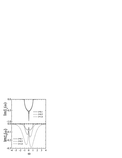
Figure 2: The imaginary part of the self-energy of conduction electrons and that of localized electrons for various values of $J$ ($V=0.5$, $E_{d}=-0.7$, $\mu=0$, $T=0.01$, $t=1$, $M$=2).

Figure 3: Density of states of conduction ($\rho_{c}(\omega)$) and localized ($\rho_{f}(\omega)$) electrons for various values of $J$ ($V=0.5$, $E_{d}=-0.7$, $\mu=0$, $T=0.01$, $t=1$, $M=2$).

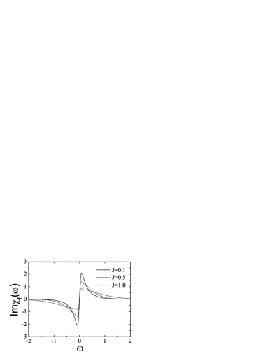
Figure 4: Local spin susceptibility for various values of $J$ ($V=0.5$, $E_{d}=-0.7$, $\mu=0$, $T=0.01$, $t=1$, $M=2$).

Figure 1 shows the phase diagram of the strongly disordered Anderson lattice model in the plane of $(V,J)$, where $V$ and $J$ are variances for the Kondo and RKKY interactions, respectively. The phase boundary is characterized by $|b|^{2}=0$, below which $|b|^{2}\not=0$ appears to cause effective hybridization between conduction electrons and localized fermions although our numerical analysis shows $\langle f^{\dagger}_{\sigma}c_{\sigma}\rangle=0$, meaning $\Sigma_{cf(fc)}(i\omega)=0$ and $G_{cf(fc)}(i\omega)=0$ in Eqs. (III.1) and (25).

In Fig. 2 one finds that the effective hybridization enhances the scattering rate of conduction electrons dramatically around the Fermi energy while the scattering rate for localized electrons becomes reduced at the resonance energy. Enhancement of the imaginary part of the conduction-electron self-energy results from the Kondo effect. In the clean situation it is given by the delta function associated with the Kondo effect Hewson_Book . This self-energy effect reflects the spectral function, shown in Fig. 3, where the pseudogap feature arises in conduction electrons while the sharply defined peak appears in localized electrons, identified with the Kondo resonance although the description of the Kondo effect differs from the clean case. Increasing the RKKY coupling, the Kondo effect is suppressed as expected. In this Kondo phase the local spin susceptibility is given by Fig. 4, displaying the typical $\omega$-linear behavior in the low frequency limit, nothing but the Fermi liquid physics for spin correlations Olivier . Increasing $J$, incoherent spin correlations are enhanced, consistent with spin liquid physics Olivier .

One can check our calculation, considering the $J=0$ limit to recover the known result. In this limit we obtain an analytic expression for $V_{c}$ at half filling ($\mu=0$)

$$V_{c}(J=0) = \sqrt{\frac{E_{d}}{2P_{c}}},$$ (31)

$$P_{c} = \int_{-1}^{1}d\omega\rho_{0}(\omega)\frac{f(\omega/T)-f(0)}{\omega},$$ (32)

where $\rho_{0}(\omega)=\frac{2}{\pi}\sqrt{1-\omega^{2}}$ is the bare density of states of conduction electrons. One can check $V_{c}(J=0)\rightarrow 0$ in the zero temperature limit because $P_{c}\rightarrow\infty$.

IV Nature of quantum criticality

IV.1 Beyond the saddle-point analysis : Non-crossing approximation

Resorting to the slave-boson mean-field approximation, we discussed the phase diagram of the strongly disordered Anderson lattice model, where a quantum phase transition appears from a spin liquid state to a dirty ”heavy-fermion” Fermi liquid phase, increasing $V/J$, the ratio of variances of the hybridization and RKKY interactions. Differentiated from the heavy-fermion quantum transition in the clean situation, the order parameter turns out to be the density of holons instead of the holon condensation. Evaluating self-energies for both conduction electrons and localized electrons, we could identify the Kondo effect from each spectral function. In addition, we obtained the local spin susceptibility consistent with the Fermi liquid physics.

The next task will be on the nature of quantum criticality between the Kondo and spin liquid phases. This question should be addressed beyond the saddle-point analysis. Introducing quantum corrections in the non-crossing approximation, justified in the $M\rightarrow\infty$ limit, we investigate the quantum critical point, where density fluctuations of holons are critical.

Releasing the slave-boson mean-field approximation to take into account holon excitations, we reach the following self-consistent equations for self-energy corrections,

$$\Sigma_{c\;\sigma\sigma^{\prime}}^{\;ab}(\tau)=\frac{V^{2}}{M}G_{f\;\sigma\sigma^{\prime}}^{\;ab}(\tau)G_{b}^{ab}(-\tau)+\frac{t^{2}}{M^{2}}\delta_{\sigma\sigma^{\prime}}G_{c\;\sigma}^{\;ab}(\tau),$$ (33)

$$\Sigma_{f\;\sigma\sigma^{\prime}}^{\;ab}(\tau) = \frac{V^{2}}{M}G_{c\;\sigma\sigma^{\prime}}^{\;ab}(\tau)G_{b}^{ab}(\tau)$$

$$+ \frac{J^{2}}{2M}\sum_{ss^{\prime}}G_{f\;ss^{\prime}}^{\;ab}(\tau)[R^{ab}_{s\sigma\sigma^{\prime}s^{\prime}}(\tau)+R^{ba}_{\sigma^{\prime}s^{\prime}s\sigma}(-\tau)],$$

$$\Sigma_{cf\;\sigma\sigma^{\prime}}^{\;\;ab}(\tau)=-\delta_{ab}\delta_{\sigma\sigma^{\prime}}\delta(\tau)\frac{V^{2}}{M}\sum_{sc}\int d\tau_{1}\langle f^{\dagger c}_{s}c^{c}_{s}\rangle G_{b}^{ca}(\tau_{1}-\tau^{\prime}),$$

$$\Sigma_{fc\;\sigma\sigma^{\prime}}^{\;\;ab}(\tau)=-\delta_{ab}\delta_{\sigma\sigma^{\prime}}\delta(\tau)\frac{V^{2}}{M}\sum_{sc}\int d\tau_{1}\langle c^{\dagger c}_{s}f^{c}_{s}\rangle G_{b}^{ac}(\tau-\tau_{1}),$$

$$\Sigma_{b}^{ab}(\tau)=\frac{V^{2}}{M}\sum_{\sigma\sigma^{\prime}}G_{f\;\sigma\sigma^{\prime}}^{\;ba}(\tau)G_{c\;\sigma^{\prime}\sigma}^{\;ba}(-\tau).$$ (37)

Since we considered the paramagnetic and replica symmetric phase, it is natural to assume such symmetries at the quantum critical point. Note that the off diagonal self-energies, $\Sigma_{cf}(i\omega_{l})$ and $\Sigma_{fc}(i\omega_{l})$, are just constants and proportional to $\langle f^{\dagger}_{\sigma}c_{\sigma}\rangle$ and $\langle c^{\dagger}_{\sigma}f_{\sigma}\rangle$, respectively. As a result, $\Sigma_{cf}(i\omega_{l})=\Sigma_{fc}(i\omega_{l})=0$ should be satisfied at the quantum critical point as the Kondo phase because of $\langle f^{\dagger}_{\sigma}c_{\sigma}\rangle=\langle c^{\dagger}_{\sigma}f_{\sigma}\rangle=0$. Then, we reach the following self-consistent equations called the non-crossing approximation

$$\Sigma_{c}(\tau) = \frac{V^{2}}{M}G_{f}(\tau)G_{b}(-\tau)+\frac{t^{2}}{M^{2}}G_{c}(\tau),$$ (38)

$$\Sigma_{f}(\tau) = \frac{V^{2}}{M}G_{c}(\tau)G_{b}(\tau)-J^{2}[G_{f}(\tau)]^{2}G_{f}(-\tau),$$ (39)

$$\Sigma_{b}(\tau) = V^{2}G_{c}(-\tau)G_{f}(\tau).$$ (40)

Local Green’s functions are given by

$$G_{c}(i\omega_{l}) = \Big{[}i\omega_{l}+\mu-\Sigma_{c}(i\omega_{l})\Big{]}^{-1},$$ (41)

$$G_{f}(i\omega_{l}) = \Big{[}i\omega_{l}-E_{d}-\lambda-\Sigma_{f}(i\omega_{l})\Big{]}^{-1},$$ (42)

$$G_{b}(i\nu_{l}) = \Big{[}i\nu_{l}-\lambda-\Sigma_{b}(i\nu_{l})\Big{]}^{-1},$$ (43)

where $\omega_{l}=(2l+1)\pi T$ is for fermions and $\nu_{l}=2l\pi T$ is for bosons.

IV.2 Asymptotic behavior at zero temperature

Calling quantum criticality, power-law scaling solutions are expected. Actually, if the second term is neglected in Eq. (39), Eqs. (39) and (40) are reduced to those of the multi-channel Kondo effect in the non-crossing approximation Hewson_Book . Power-law solutions are well known in the regime of $1/T_{K}\ll\tau\ll\beta=1/T\rightarrow\infty$, where $T_{K}=D[\Gamma_{c}/\pi D]^{1/M}\exp[\pi E_{d}/M\Gamma_{c}]$ is an effective Kondo temperature Tien_Kim with the conduction bandwidth $D$ and effective hybridization $\Gamma_{c}=\pi\rho_{c}\frac{V^{2}}{M}$. In the presence of the RKKY interaction [the second term in Eq. (39)], the effective hybridization will be reduced, where $\Gamma_{c}$ is replaced with $\Gamma_{c}^{J}\approx\pi\rho_{c}(\frac{V^{2}}{M}-J^{2})$.

Our power-law ansatz is as follows

$$G_{c} = \frac{A_{c}}{\tau^{\Delta_{c}}},$$ (44)

$$G_{f} = \frac{A_{f}}{\tau^{\Delta_{f}}},$$ (45)

$$G_{b} = \frac{A_{b}}{\tau^{\Delta_{b}}},$$ (46)

where $A_{c}$, $A_{f}$, and $A_{b}$ are positive numerical constants. In the frequency space these are

$$G_{c}(\omega) = A_{c}C_{\Delta_{c}-1}\omega^{\Delta_{c}-1},$$ (47)

$$G_{f}(\omega) = A_{f}C_{\Delta_{f}-1}\omega^{\Delta_{f}-1},$$ (48)

$$G_{b}(\omega) = A_{b}C_{\Delta_{b}-1}\omega^{\Delta_{b}-1},$$ (49)

where $C_{\Delta_{c,f,b}}=\int_{-\infty}^{\infty}dx\frac{e^{ix}}{x^{\Delta_{c,f,b}+1}}.$

Inserting Eqs. (47)-(49) into Eqs. (38)-(40), we obtain scaling exponents of $\Delta_{c}$, $\Delta_{f}$, and $\Delta_{b}$. In appendix C-1 we show how to find such critical exponents in a detail. Two fixed points are allowed. One coincides with the multi-channel Kondo effect, given by $\Delta_{c}=1$, and $\Delta_{f}=\frac{M}{M+1}$, $\Delta_{b}=\frac{1}{M+1}$ with $M=2$, where contributions from spin fluctuations to self-energy corrections are irrelevant, compared with holon fluctuations. The other is $\Delta_{c}=1$ and $\Delta_{f}=\Delta_{b}=\frac{1}{2}$, where spin correlations are critical as much as holon fluctuations.

One can understand the critical exponent $\Delta_{f}=1/2$ as the proximity of the spin liquid physics Sachdev_SG . Considering the $V\rightarrow 0$ limit, we obtain the scaling exponents of $\Delta_{c}=1$ and $\Delta_{f}=1/2$ from the scaling equations (102) and (103). Thus, $G_{c}(\omega)\sim\mbox{sgn}(\omega)$ and $G_{f}(\omega)\sim 1/\sqrt{\omega}$ result for $\omega\rightarrow 0$. In this respect both spin fluctuations and holon excitations are critical as equal strength at this quantum critical point.

IV.3 Finite temperature scaling behavior

We solve Eqs. (38)-(40) in the regime $\tau,\beta\gg 1/T_{K}$ with arbitrary $\tau/\beta$, where the scaling ansatz at zero temperature is generalized as follows

$$G_{c}(\tau) = A_{c}\beta^{-\Delta_{c}}g_{c}\Big{(}\frac{\tau}{\beta}\Big{)},$$ (50)

$$G_{f}(\tau) = A_{f}\beta^{-\Delta_{f}}g_{f}\Big{(}\frac{\tau}{\beta}\Big{)},$$ (51)

$$G_{b}(\tau) = A_{b}\beta^{-\Delta_{b}}g_{b}\Big{(}\frac{\tau}{\beta}\Big{)}.$$ (52)

$$g_{\alpha}(x)=\bigg{(}\frac{\pi}{\sin(\pi x)}\bigg{)}^{\Delta_{\alpha}}$$ (53)

with $\alpha=c,f,b$ is the scaling function at finite temperatures. In the frequency space we obtain

$$G_{c}(i\omega_{l}) = A_{c}\beta^{1-\Delta_{c}}\Phi_{c}(i\bar{\omega}_{l}),$$ (54)

$$G_{f}(i\omega_{l}) = A_{f}\beta^{1-\Delta_{f}}\Phi_{f}(i\bar{\omega}_{l}),$$ (55)

$$G_{b}(i\nu_{l}) = A_{c}\beta^{1-\Delta_{b}}\Phi_{b}(i\bar{\nu}_{l}),$$ (56)

where $\bar{\omega}_{l}=(2l+1)\pi$, $\bar{\nu}_{l}=2l\pi$, and

$$\Phi_{\alpha}(i\bar{x})=\int_{0}^{1}dte^{i\bar{x}t}g_{\alpha}(t).$$ (57)

Inserting Eqs. (54)-(56) into Eqs. (38)-(40), we find two fixed points, essentially the same as the case of $T=0$. But, scaling functions of $\Phi_{c}(i\bar{\omega}_{l})$, $\Phi_{f}(i\bar{\omega}_{l})$, and $\Phi_{b}(i\bar{\omega}_{l})$ are somewhat complicated. All scaling functions are derived in appendix C-2.

IV.4 Spin susceptibility

We evaluate the local spin susceptibility, given by

$$\chi(\tau) = G_{f}(\tau)G_{f}(-\tau),$$ (58)

$$= A_{f}^{2}\beta^{-2\Delta_{f}}\bigg{(}\frac{\pi}{\sin(\pi\tau/\beta)}\bigg{)}^{2\Delta_{f}}.$$

The imaginary part of the spin susceptibility $\chi^{{}^{\prime\prime}}(\omega)={\rm Im}\;\chi(\omega+i0^{+})$ can be found from

$$\chi(\tau)=\int\frac{d\omega}{\pi}\frac{e^{-\tau\omega}}{1-e^{-\beta\omega}}\chi^{{}^{\prime\prime}}(\omega).$$ (59)

Inserting the scaling ansatz

$$\chi^{{}^{\prime\prime}}(\omega)=A_{f}^{2}\beta^{1-2\Delta_{f}}\phi\Big{(}\frac{\omega}{T}\Big{)}$$ (60)

into Eq. (59) with Eq. (58), we obtain

$$\int\frac{dx}{\pi}\frac{e^{-x\tau/\beta}}{1-e^{-x}}\phi(x)=\bigg{(}\frac{\pi}{\sin(\pi\tau/\beta)}\bigg{)}^{2\Delta_{f}}.$$ (61)

Changing the variable $t=i(\tau/\beta-1/2)$, we obtain

$$\int\frac{dx}{\pi}e^{ixt}\frac{\phi(x)}{e^{x}-e^{-x}}=\bigg{(}\frac{\pi}{\cosh(\pi t)}\bigg{)}^{2\Delta_{f}}.$$ (62)

As a result, we find the scaling function

$$\phi(x)=2(2\pi)^{2\Delta_{f}-1}\sinh\Big{(}\frac{x}{2}\Big{)}\frac{\Gamma(\Delta_{f}+ix/2\pi)\Gamma(\Delta_{f}-ix/2\pi)}{\Gamma(2\Delta_{f})}.$$

This coincides with the spin spectrum of the spin liquid state when $V=0$ Olivier .

IV.5 Discussion : Deconfined local quantum criticality

The local quantum critical point characterized by $\Delta_{c}=1$ and $\Delta_{f}=\Delta_{b}=1/2$ is the genuine critical point in the spin-liquid to local Fermi-liquid transition because such a fixed point can be connected to the spin liquid state ($\Delta_{c}=1$ and $\Delta_{f}=1/2$) naturally. This fixed point results from the fact that the spinon self-energy correction from RKKY spin fluctuations is exactly the same order as that from critical holon excitations. It is straightforward to see that the critical exponent of the local spin susceptibility is exactly the same as that of the local charge susceptibility ($2\Delta_{f}=2\Delta_{b}=1$), proportional to $1/\tau$. Since the spinon spin-density operator differs from the holon charge-density operator in the respect of symmetry at the lattice scale, the same critical exponent implies enhancement of the original symmetry at low energies. The symmetry enhancement sometimes allows a topological term, which assigns a nontrivial quantum number to a topological soliton, identified with an excitation of quantum number fractionalization. This mathematical structure is actually realized in an antiferromagnetic spin chain Tsvelik_Book , generalized into the two dimensional case Senthil_DQCP ; Tanaka_SO5 .

We propose the following local field theory in terms of physically observable fields

$$Z_{eff} = \int D\bm{\Psi}^{a}(\tau)\delta\Bigl{(}|\bm{\Psi}^{a}(\tau)|^{2}-1\Bigr{)}e^{-\mathcal{S}_{eff}},$$

$$\mathcal{S}_{eff} = -\frac{g^{2}}{2M}\int_{0}^{\beta}d\tau\int_{0}^{\beta}d\tau^{\prime}\bm{\Psi}^{aT}(\tau)\bm{\Upsilon}^{ab}(\tau-\tau^{\prime})\bm{\Psi}^{b}(\tau^{\prime})$$ (64)

$$+ \mathcal{S}_{top},$$

where

$$\bm{\Psi}^{a}(\tau)=\left(\begin{array}[]{c}\bm{S}^{a}(\tau)\\ \rho^{a}(\tau)\end{array}\right)$$ (67)

represents an $O(4)$ vector, satisfying the constraint of the delta function. $\bm{\Upsilon}^{ab}(\tau-\tau^{\prime})$ determines dynamics of the $O(4)$ vector, resulting from spin and holon dynamics in principle. However, it is extremely difficult to derive Eq. (64) from Eq. (4) because the density part for the holon field in Eq. (64) cannot result from Eq. (4) in a standard way. What we have shown is that the renormalized dynamics for the O(4) vector field follows $1/\tau$ asymptotically, where $\tau$ is the imaginary time. This information should be introduced in $\bm{\Upsilon}^{ab}(\tau-\tau^{\prime})$. $g\propto V/J$ is an effective coupling constant, and $\mathcal{S}_{top}$ is a possible topological term.

One can represent the O(4) vector generally as follows

$$\bm{\Psi}^{a}:\tau\longrightarrow\Bigl{(}\sin\theta^{a}(\tau)\sin\phi^{a}(\tau)\cos\varphi^{a}(\tau),\sin\theta^{a}(\tau)\sin\phi^{a}(\tau)\sin\varphi^{a}(\tau),\sin\theta^{a}(\tau)\cos\phi^{a}(\tau),\cos\theta^{a}(\tau)\Bigr{)},$$ (68)

where $\theta^{a}(\tau),\phi^{a}(\tau),\varphi^{a}(\tau)$ are three angle coordinates for the O(4) vector. It is essential to observe that the target manifold for the O(4) vector is not a simple sphere type, but more complicated because the last component of the O(4) vector is the charge density field, where three spin components lie in $-1\leq S^{a}_{x}(\tau),S^{a}_{y}(\tau),S^{a}_{z}(\tau)\leq 1$ while the charge density should be positive, $0\leq\rho^{a}(\tau)\leq 1$. This leads us to identify the lower half sphere with the upper half sphere. Considering that $\sin\theta^{a}(\tau)$ can be folded on $\pi/2$, we are allowed to construct our target manifold to have a periodicity, given by $\bm{\Psi}^{a}(\theta^{a},\phi^{a},\varphi^{a})=\bm{\Psi}^{a}(\pi-\theta^{a},\phi^{a},\varphi^{a})$. This folded space allows a nontrivial topological excitation.

Suppose the boundary configuration of $\bm{\Psi}^{a}(0,\phi^{a},\varphi^{a};\tau=0)$ and $\bm{\Psi}^{a}(\pi,\phi^{a},\varphi^{a};\tau=\beta)$, connected by $\bm{\Psi}^{a}(\pi/2,\phi^{a},\varphi^{a};0<\tau<\beta)$. Interestingly, this configuration is topologically distinguishable from the configuration of $\bm{\Psi}^{a}(0,\phi^{a},\varphi^{a};\tau=0)$ and $\bm{\Psi}^{a}(0,\phi^{a},\varphi^{a};\tau=\beta)$ with $\bm{\Psi}^{a}(\pi/2,\phi^{a},\varphi^{a};0<\tau<\beta)$ because of the folded structure. The second configuration shrinks to a point while the first excitation cannot, identified with a topologically nontrivial excitation. This topological excitation carries a spin quantum number $1/2$ in its core, given by $\bm{\Psi}^{a}(\pi/2,\phi^{a},\varphi^{a};0<\tau<\beta)=\Bigl{(}\sin\phi^{a}(\tau)\cos\varphi^{a}(\tau),\sin\phi^{a}(\tau)\sin\varphi^{a}(\tau),\cos\phi^{a}(\tau),0\Bigr{)}$. This is the spinon excitation, described by an O(3) nonlinear $\sigma$ model with the nontrivial spin correlation function $\bm{\Upsilon}^{ab}(\tau-\tau^{\prime})$, where the topological term is reduced to the single spin Berry phase term in the instanton core.

In this local impurity picture the local Fermi liquid phase is described by gapping of instantons while the spin liquid state is characterized by condensation of instantons. Of course, the low dimensionality does not allow condensation, resulting in critical dynamics for spinons. This scenario clarifies the Landau-Ginzburg-Wilson forbidden duality between the Kondo singlet and the critical local moment for the impurity state, allowed by the presence of the topological term.

If the symmetry enhancement does not occur, the effective local field theory will be given by

$$Z_{eff} = \int D\bm{S}^{a}(\tau)D\rho^{a}(\tau)e^{-\mathcal{S}_{eff}},$$

$$\mathcal{S}_{eff} = -\int_{0}^{\beta}d\tau\int_{0}^{\beta}d\tau^{\prime}\Bigl{\{}\frac{V^{2}}{2M}\rho^{a}(\tau)\chi^{ab}(\tau-\tau^{\prime})\rho^{b}(\tau^{\prime})$$ (69)

$$+ \frac{J^{2}}{2M}\bm{S}^{a}(\tau)R^{ab}(\tau-\tau^{\prime})\bm{S}^{b}(\tau^{\prime})\Bigr{\}}+\mathcal{S}_{B}$$

with the single-spin Berry phase term

$$\mathcal{S}_{B}=-2\pi iS\int_{0}^{1}du\int_{0}^{\beta}d\tau\frac{1}{4\pi}\bm{S}^{a}(u,\tau)\partial_{u}\bm{S}^{a}(u,\tau)\times\partial_{\tau}\bm{S}^{a}(u,\tau),$$

where charge dynamics $\chi^{ab}(\tau-\tau^{\prime})$ will be different from spin dynamics $R^{ab}(\tau-\tau^{\prime})$. This will not allow the spin fractionalization for the critical impurity dynamics, where the instanton construction is not realized due to the absence of the symmetry enhancement.

V Summary

In this paper we have studied the Anderson lattice model with strong randomness in both hybridization and RKKY interactions, where their average values are zero. In the absence of random hybridization quantum fluctuations in spin dynamics cause the spin glass phase unstable at finite temperatures, giving rise to the spin liquid state, characterized by the $\omega/T$ scaling spin spectrum consistent with the marginal Fermi-liquid phenomenology Sachdev_SG . In the absence of random RKKY interactions the Kondo effect arises Kondo_Disorder , but differentiated from that in the clean case. The dirty ”heavy fermion” phase in the strongly disordered Kondo coupling is characterized by a finite density of holons instead of the holon condensation. But, effective hybridization exists indeed, causing the Kondo resonance peak in the spectral function. As long as variation of the effective Kondo temperature is not so large, this disordered Kondo phase is identified with the local Fermi liquid state because essential physics results from single impurity dynamics, differentiated from the clean lattice model.

Taking into account both random hybridization and RKKY interactions, we find the quantum phase transition from the spin liquid state to the local Fermi liquid phase at the critical $(V_{c},J_{c})$. Each phase turns out to be adiabatically connected with each limit, i.e., the spin liquid phase when $V=0$ and the local Fermi liquid phase when $J=0$, respectively. Actually, we have checked this physics, considering the local spin susceptibility and the spectral function for localized electrons.

In order to investigate quantum critical physics, we introduce quantum corrections from critical holon fluctuations in the non-crossing approximation beyond the slave-boson mean-field analysis. We find two kinds of power-law scaling solutions for self-energy corrections of conduction electrons, spinons, and holons. The first solution turns out to coincide with that of the multi-channel Kondo effect, where effects of spin fluctuations are sub-leading, compared with critical holon fluctuations. In this respect this quantum critical point is characterized by breakdown of the Kondo effect while spin fluctuations can be neglected. On the other hand, the second scaling solution shows that both holon excitations and spinon fluctuations are critical as the same strength, reflected in the fact that the density-density correlation function of holons has the exactly the same critical exponent as the local spin-spin correlation function of spinons.

We argued that the second quantum critical point implies an enhanced emergent symmetry from O(3)$\times$O(2) (spin$\otimes$charge) to O(4) at low energies, forcing us to construct an O(4) nonlinear $\sigma$ model on the folded target manifold as an effective field theory for this disorder-driven local quantum critical point. Our effective local field theory identifies spinons with instantons, describing the local Fermi-liquid to spin-liquid transition as the condensation transition of instantons although dynamics of instantons remains critical in the spin liquid state instead of condensation due to low dimensionality. This construction completes novel duality between the Kondo and critical local moment phases in the strongly disordered Anderson lattice model.

We explicitly checked that the similar result can be found in the extended DMFT for the clean Kondo lattice model, where two fixed point solutions are allowed EDMFT_Spin ; EDMFT_NCA . One is the same as the multi-channel Kondo effect and the other is essentially the same as the second solution in this paper. In this respect we believe that the present scenario works in the extended DMFT framework although applicable to only two spatial dimensions EDMFT .

One may suspect the applicability of the DMFT framework for this disorder problem. However, the hybridization term turns out to be exactly local in the case of strong randomness while the RKKY term is safely approximated to be local for the spin liquid state, expected to be stable against the spin glass phase in the case of quantum spins. This situation should be distinguished from the clean case, where the DMFT approximation causes several problems such as the stability of the spin liquid state EDMFT_Rosch and strong dependence of the dimension of spin dynamics EDMFT .

Appendix A Derivation of Eq. (3) from Eq. (1) in the Replica method

The replica trick SG_Review has been utilized for the disorder average, given by the following identity

$$\overline{\ln Z}=\lim_{n\rightarrow 0}\frac{\overline{Z^{n}}-1}{n},$$ (70)

where $\overline{\mathcal{O}}$ means the disorder average of an operator $\mathcal{O}$. $Z^{n}$ is the replicated partition function

$$Z^{n}=\int\mathcal{D}c_{i\sigma}^{a}\mathcal{D}d_{i\sigma}^{a}e^{-S_{n}},$$ (71)

where the corresponding replica action is

$$S_{n} =\int\limits_{0}^{\beta}d\tau\Bigl{[}\sum_{i\sigma a}c^{\dagger a}_{i\sigma}(\tau)(\partial_{\tau}-\mu)c^{a}_{i\sigma}(\tau)-\sum_{ij\sigma a}t_{ij}c^{\dagger a}_{i\sigma}(\tau)c^{a}_{j\sigma}(\tau)$$ (72)

$$+\sum_{i\sigma a}d^{\dagger a}_{i\sigma}(\tau)(\partial_{\tau}+E_{d})d^{a}_{i\sigma}(\tau)+\sum_{ija}J_{ij}\mathbf{S}^{a}_{i}(\tau)\cdot\mathbf{S}^{a}_{j}(\tau)$$

$$+\sum_{i\sigma a}(V_{i}c^{\dagger a}_{i\sigma}(\tau)d^{a}_{i\sigma}(\tau)+{\rm H.c.})\Bigr{]}$$

with the spin index $\sigma=1,...,M$ and the replica index $a=1,...,n$.

The disorder average for the replicated partition function is straightforward, given by

$$\overline{Z^{n}}=\int d\varepsilon_{i}P[\varepsilon_{i}]\int\mathcal{D}c_{i\sigma}^{a}\mathcal{D}d_{i\sigma}^{a}e^{-S_{n}},$$ (73)

where $P[\varepsilon_{i}]$ is the Gaussian distribution function with $\int d\varepsilon_{i}P[\varepsilon_{i}]=1$. Performing integrals for random variables, we obtain an effective action Eq. (3).

Appendix B Derivation of Eq. (4) from Eq. (3) in the cavity method

We solve the replicated Anderson lattice model Eq. (3) in the DMFT approximation. We apply the cavity method for the DMFT mapping DMFT_Review

$$\overline{S}_{n}=\bar{S}_{n}^{0}+\Delta\bar{S}_{n}+\bar{S}_{n}^{(0)},$$ (74)

where $\bar{S}_{n}^{0}$ is the part of the action at a particular site $0$, $\Delta\bar{S}_{n}$ is the part of the action connecting the site $0$ with other sites, given by

$$\bar{S}_{n}^{0}=\int_{0}^{\beta}d\tau\sum_{\sigma a}\Bigl{\{}c^{\dagger a}_{0\sigma}(\tau)(\partial_{\tau}-\mu)c^{a}_{0\sigma}(\tau)+d^{\dagger a}_{0\sigma}(\tau)(\partial_{\tau}+E_{d})d^{a}_{0\sigma}(\tau)\Bigr{\}}$$

$$-\frac{V^{2}}{2M}\int_{0}^{\beta}d\tau\int_{0}^{\beta}d\tau^{\prime}\sum_{\sigma\sigma^{\prime}ab}\big{[}c^{\dagger a}_{0\sigma}(\tau)d^{a}_{0\sigma}(\tau)+d^{\dagger a}_{0\sigma}(\tau)c^{a}_{0\sigma}(\tau)\big{]}\big{[}c^{\dagger b}_{0\sigma^{\prime}}(\tau^{\prime})d^{b}_{0\sigma^{\prime}}(\tau^{\prime})+d^{\dagger b}_{0\sigma^{\prime}}(\tau^{\prime})c^{b}_{0\sigma^{\prime}}(\tau^{\prime})\big{]},$$ (75)

$$\Delta\bar{S}_{n}=-\int_{0}^{\beta}d\tau\sum_{i\sigma a}\Bigl{\{}c^{\dagger a}_{0\sigma}(\tau)t_{0i}c^{a}_{i\sigma}(\tau)+c^{\dagger a}_{i\sigma}(\tau)t_{i0}c^{a}_{0\sigma}(\tau)\Bigr{\}}$$

$$-\frac{J^{2}}{2zM}\int_{0}^{\beta}d\tau\int_{0}^{\beta}d\tau^{\prime}\sum_{iab}\mathbf{S}^{a}_{0}(\tau)\cdot\mathbf{S}^{a}_{i}(\tau)\;\;\mathbf{S}^{b}_{0}(\tau^{\prime})\cdot\mathbf{S}^{b}_{i}(\tau^{\prime}),$$

respectively, and $\bar{S}_{n}^{(0)}$ is the rest part of the action.

The partition function can be expanded as follows

$$\overline{Z^{n}} = \int\mathcal{D}c_{i\sigma}^{a}\mathcal{D}d_{i\sigma}^{a}\exp(-\bar{S}_{n}^{0}-\bar{S}_{n}^{(0)}-\Delta\bar{S}_{n})$$ (77)

$$= \int\mathcal{D}c^{a}_{0\sigma}\mathcal{D}d^{a}_{0\sigma}\frac{e^{-\bar{S}_{n}^{0}}}{\bar{Z^{n}}^{(0)}}\Big{[}1-\int_{0}^{\beta}d\tau\langle\Delta\mathcal{L}(\tau)\rangle^{(0)}$$

$$+ \frac{1}{2!}\int_{0}^{\beta}d\tau\int_{0}^{\beta}d\tau^{\prime}\langle T_{\tau}\Delta\mathcal{L}(\tau)\Delta\mathcal{L}(\tau^{\prime})\rangle^{(0)}+\cdots\Big{]},$$

where

$$\langle\mathcal{O}\rangle^{(0)}\equiv\frac{1}{\bar{Z^{n}}^{(0)}}\int\mathcal{D}c_{i\not=0\sigma}^{a}\mathcal{D}d_{i\not=0\sigma}^{a}\mathcal{O}\exp(-\bar{S}_{n}^{(0)})$$

with $\bar{Z^{n}}^{(0)}=\int\mathcal{D}c_{i\not=0\sigma}^{a}\mathcal{D}d_{i\not=0\sigma}^{a}\exp(-\bar{S}_{n}^{(0)})$ and $\Delta\bar{S}_{n}=\int_{0}^{\beta}d\tau\Delta\mathcal{L}(\tau)$.

The non-trivial term in the first order is given by

$$\int_{0}^{\beta}d\tau\langle\Delta\mathcal{L}(\tau)\rangle^{(0)} = -\frac{J^{2}}{2zM}\int_{0}^{\beta}d\tau\int_{0}^{\beta}d\tau^{\prime}\sum_{iab}\langle T_{\tau}\mathbf{S}^{a}_{0}(\tau)\cdot\mathbf{S}^{a}_{i}(\tau)\;\;\mathbf{S}^{b}_{0}(\tau^{\prime})\cdot\mathbf{S}^{b}_{i}(\tau^{\prime})\rangle^{(0)}$$ (78)

$$= -\frac{J^{2}}{2M}\int_{0}^{\beta}d\tau\int_{0}^{\beta}d\tau^{\prime}\sum_{ab}\sum_{\alpha\beta\gamma\delta}S^{a}_{0\alpha\beta}(\tau)R^{ab\;(0)}_{\beta\alpha\gamma\delta}(\tau-\tau^{\prime})S^{b}_{0\gamma\delta}(\tau^{\prime}),$$

where $R^{ab\;(0)}_{\beta\alpha\gamma\delta}(\tau-\tau^{\prime})=\langle T_{\tau}S^{a}_{\beta\alpha}(\tau)S^{b}_{\gamma\delta}(\tau^{\prime})\rangle^{(0)}$. The second order term is

$$\int_{0}^{\beta}d\tau\int_{0}^{\beta}d\tau^{\prime}\langle T_{\tau}\Delta\mathcal{L}(\tau)\Delta\mathcal{L}(\tau^{\prime})\rangle^{(0)} = \int_{0}^{\beta}d\tau\int_{0}^{\beta}d\tau^{\prime}\sum_{ij\sigma ab}\langle T_{\tau}c^{\dagger a}_{0\sigma}(\tau)t_{0i}c^{a}_{i\sigma}(\tau)c^{\dagger b}_{j\sigma}(\tau^{\prime})t_{j0}c^{b}_{0\sigma}(\tau^{\prime})\rangle^{(0)}$$ (79)

$$= -\int_{0}^{\beta}d\tau\int_{0}^{\beta}d\tau^{\prime}\sum_{ij\sigma ab}c^{\dagger a}_{0\sigma}(\tau)t_{0i}G^{ab\;(0)}_{c\;ij\sigma\sigma}(\tau-\tau^{\prime})t_{j0}c^{b}_{0\sigma}(\tau^{\prime}),$$

where $G^{ab\;(0)}_{c\;ij\sigma\sigma}(\tau-\tau^{\prime})=-\langle T_{\tau}c^{a}_{i\sigma}(\tau)c^{\dagger b}_{j\sigma}(\tau^{\prime})\rangle^{(0)}$. One can easily verify that all higher order expansions in Eq. (77) vanish in the limit $z\rightarrow\infty$, which is at the heart of the DMFT approximation DMFT_Review .

In the $z\rightarrow\infty$ Bethe lattice we perform further simplificationDMFT_Review

$$G^{ab\;(0)}_{c\;ij\sigma\sigma}(\tau)=\delta_{ij}G^{ab}_{c\;ii\sigma}(\tau)\equiv\delta_{ij}G^{ab}_{c\;\sigma\sigma}(\tau),$$

$$R^{ab\;(0)}_{\beta\alpha\gamma\delta}(\tau)=R^{ab}_{\beta\alpha\gamma\delta}(\tau).$$ (80)

As a result, we reach an effective single-site action Eq. (4) called the DMFT approximation.

Appendix C Derivation of critical exponents, $\Delta_{c}$, $\Delta_{f}$, and $\Delta_{b}$

C.1 At zero temperature

Inserting Eqs. (47)-(49) into Eqs. (38)-(40), we obtain

$$\Sigma_{c}(\omega) = \frac{V^{2}}{M}A_{f}A_{b}C_{\Delta_{f}+\Delta_{b}-1}\omega^{\Delta_{f}+\Delta_{b}-1}$$ (81)

$$+ \frac{t^{2}}{M^{2}}A_{c}C_{\Delta_{c}-1}\omega^{\Delta_{c}-1},$$

$$\Sigma_{f}(\omega) = \frac{V^{2}}{M}A_{c}A_{b}C_{\Delta_{c}+\Delta_{b}-1}\omega^{\Delta_{c}+\Delta_{b}-1}$$ (82)

$$- J^{2}A_{f}^{3}C_{3\Delta_{f}-1}\omega^{3\Delta_{f}-1},$$

$$\Sigma_{b}(\omega) = V^{2}A_{c}A_{f}C_{\Delta_{c}+\Delta_{f}-1}\omega^{\Delta_{c}+\Delta_{f}-1}.$$ (83)

It is naturally expected

$$\Sigma_{f}(0^{+}) = -E_{d}-\lambda,$$ (84)

$$\Sigma_{b}(0^{+}) = -\lambda$$ (85)

for power-law solutions at zero temperature.

Combined with the Dyson equations (41)-(43), we reach the following equations

$$\frac{1}{A_{c}C_{\Delta_{c}-1}}\omega^{1-\Delta_{c}} = \omega+\mu-\frac{V^{2}}{M}A_{f}A_{b}C_{\Delta_{f}+\Delta_{b}-1}\omega^{\Delta_{f}+\Delta_{b}-1}$$ (86)

$$- \frac{t^{2}}{M^{2}}A_{c}C_{\Delta_{c}-1}\omega^{\Delta_{c}-1},$$

$$\frac{1}{A_{f}C_{\Delta_{f}-1}}\omega^{1-\Delta_{f}} = -\frac{V^{2}}{M}A_{c}A_{b}C_{\Delta_{c}+\Delta_{b}-1}\omega^{\Delta_{c}+\Delta_{b}-1}$$ (87)

$$+ J^{2}A_{f}^{3}C_{3\Delta_{f}-1}\omega^{3\Delta_{f}-1},$$

$$\frac{1}{A_{b}C_{\Delta_{b}-1}}\omega^{1-\Delta_{b}} = -V^{2}A_{c}A_{f}C_{\Delta_{c}+\Delta_{f}-1}\omega^{\Delta_{c}+\Delta_{f}-1}.$$ (88)

The last equation gives

$$\Delta_{c}+\Delta_{f}+\Delta_{b}=2.$$ (89)

Comparing this with the first equation, we get

$$\Delta_{c}=1.$$ (90)

The second equation gives two possible solutions. One is again $\Delta_{c}+\Delta_{f}+\Delta_{b}=2$, and the other $\Delta_{f}=\Delta_{b}=1/2$. We can find the first solution by equating the coefficients in Eqs. (87)-(88) and obtain

$$\frac{1}{C_{\Delta_{f}-1}C_{\Delta_{b}}} = -\frac{V^{2}}{M}A_{c}A_{f}A_{b},$$ (91)

$$\frac{1}{C_{\Delta_{b}-1}C_{\Delta_{f}}} = -V^{2}A_{c}A_{f}A_{b}.$$ (92)

These two equations result in

$$C_{\Delta_{f}-1}C_{\Delta_{b}}=MC_{\Delta_{b}-1}C_{\Delta_{f}}.$$

Using the property of $C_{\Delta-1}=\Delta C_{\Delta}$, we obtain

$$\Delta_{f}=M\Delta_{b}.$$

As a result, the first solution is

$$\Delta_{f} = \frac{M}{M+1},$$ (93)

$$\Delta_{b} = \frac{1}{M+1},$$ (94)

exactly the same as those of the multi-channel Kondo effect.

C.2 At finite temperatures

Inserting Eqs. (54)-(56) into Eqs. (38)-(40), we obtain

$$\Sigma_{c}(i\omega_{l}) = \frac{V^{2}}{M}A_{f}A_{b}\beta^{1-\Delta_{f}-\Delta_{b}}\Psi_{fb}(i\bar{\omega}_{l})$$ (95)

$$+ \frac{t^{2}}{M^{2}}\beta^{1-\Delta_{c}}\Phi_{c}(i\bar{\omega}_{l}),$$

$$\Sigma_{f}(i\omega_{l}) = \frac{V^{2}}{M}A_{c}A_{b}\beta^{1-\Delta_{c}-\Delta_{b}}\Psi_{cb}(i\bar{\omega}_{l})$$ (96)

$$- J^{2}A_{f}^{3}\beta^{1-3\Delta_{f}}\Psi_{fff}(i\bar{\omega}_{l}),$$

$$\Sigma_{b}(i\nu_{l}) = V^{2}A_{c}A_{f}\beta^{1-\Delta_{c}-\Delta_{f}}\Psi_{cf}(i\bar{\nu}_{l}),$$ (97)

where

$$\Psi_{fb}(i\bar{\omega}_{l}) = \int_{0}^{1}dte^{i\bar{\omega}_{l}t}g_{f}(t)g_{b}(-t),$$ (98)

$$\Psi_{cb}(i\bar{\omega}_{l}) = \int_{0}^{1}dte^{i\bar{\omega}_{l}t}g_{c}(t)g_{b}(t),$$ (99)

$$\Psi_{fff}(i\bar{\omega}_{l}) = \int_{0}^{1}dte^{i\bar{\omega}_{l}t}[g_{f}(t)]^{2}g_{f}(-t),$$ (100)

$$\Psi_{cf}(i\bar{\nu}_{l}) = \int_{0}^{1}dte^{i\bar{\nu}_{l}t}g_{c}(-t)g_{f}(t).$$ (101)

Using the Dyson equations, we obtain the final self-consistency expressions

$$A_{c}^{-1}\Phi_{c}^{-1}(i\bar{\omega}_{l}) = [i\bar{\omega}_{l}T+\mu]\beta^{1-\Delta_{c}}-\frac{V^{2}}{M}A_{f}A_{b}\beta^{2-\Delta_{c}-\Delta_{f}-\Delta_{b}}\Psi_{fb}(i\bar{\omega}_{l})-\frac{t^{2}}{M^{2}}\beta^{2-2\Delta_{c}}\Phi_{c}(i\bar{\omega}_{l}),$$ (102)

$$A_{f}^{-1}\Phi_{f}^{-1}(i\bar{\omega}_{l}) = i\bar{\omega}_{l}\beta^{-\Delta_{f}}-[E_{d}+\lambda-\Sigma_{f}(i\omega_{0})]\beta^{1-\Delta_{f}}-\frac{V^{2}}{M}A_{c}A_{b}\beta^{2-\Delta_{c}-\Delta_{f}-\Delta_{b}}[\Psi_{cb}(i\bar{\omega}_{l})-\Psi_{cb}(i\bar{\omega}_{0})]$$ (103)

$$+ J^{2}A_{f}^{3}\beta^{2-4\Delta_{f}}[\Psi_{fff}(i\bar{\omega}_{l})-\Psi_{fff}(i\bar{\omega}_{0})],$$

$$A_{b}^{-1}\Phi_{b}^{-1}(i\bar{\nu}_{l}) = i\bar{\nu}_{l}\beta^{-\Delta_{b}}-[\lambda-\Sigma_{b}(i\bar{\nu}_{0})]\beta^{1-\Delta_{b}}+V^{2}A_{c}A_{f}\beta^{2-\Delta_{c}-\Delta_{f}-\Delta_{b}}[\Psi_{cf}(i\bar{\nu}_{l})-\Psi_{cf}(i\bar{\nu}_{0})].$$ (104)

As the zero temperature case, we obtain two power-law solutions, comparing the powers of $\beta$ terms. One is

$$\Delta_{c}=1,$$ (105)

$$\Delta_{f}+\Delta_{b}=1,$$ (106)

with $\Delta_{f}>1/2$. The other solution is

$$\Delta_{c}=1,$$ (107)

$$\Delta_{f}=\Delta_{b}=1/2.$$ (108)

Note that Eqs. (102) and (104) are same for both solutions. Only Eq. (103) distinguishes these two solutions.

Inserting Eq. (53) into Eqs. (57), (98)-(99), we obtain

$$\Phi_{c}(i\bar{\omega}_{l}) = i\pi\;{\rm sgn}(\bar{\omega}_{l}),$$ (109)

$$\Phi_{f}(i\bar{\omega}_{l}) = (2\pi)^{\Delta_{f}}i(-1)^{l}\frac{\Gamma(1-\Delta_{f})}{\Gamma(1-\frac{\Delta_{f}}{2}+\frac{\bar{\omega}_{l}}{2\pi})\Gamma(1-\frac{\Delta_{f}}{2}-\frac{\bar{\omega}_{l}}{2\pi})},$$ (110)

$$\Phi_{b}(i\bar{\nu}_{l}) = (2\pi)^{\Delta_{b}}(-1)^{l}\frac{\Gamma(1-\Delta_{b})}{\Gamma(1-\frac{\Delta_{b}}{2}+\frac{\bar{\nu}_{l}}{2\pi})\Gamma(1-\frac{\Delta_{b}}{2}-\frac{\bar{\nu}_{l}}{2\pi})}$$ (111)

and

$$\Psi_{fb}(i\bar{\omega}_{l}) = i\pi\;{\rm sgn}(\bar{\omega}_{l}),$$ (112)

$$\Psi_{cb}(i\bar{\omega}_{l}) = (2\pi)^{\Delta_{b}+1}i(-1)^{l}\frac{\Gamma(-\Delta_{b})}{\Gamma(\frac{1}{2}-\frac{\Delta_{b}}{2}+\frac{\bar{\omega}_{l}}{2\pi})\Gamma(\frac{1}{2}-\frac{\Delta_{b}}{2}-\frac{\bar{\omega}_{l}}{2\pi})},$$ (113)

$$\Psi_{fff}(i\bar{\omega}_{l}) = (2\pi)^{3\Delta_{f}}i(-1)^{l}\frac{\Gamma(1-3\Delta_{f})}{\Gamma(1-\frac{3\Delta_{f}}{2}+\frac{\bar{\omega}_{l}}{2\pi})\Gamma(1-\frac{3\Delta_{f}}{2}-\frac{\bar{\omega}_{l}}{2\pi})},$$ (114)

$$\Psi_{cf}(i\bar{\nu}_{l}) = (2\pi)^{\Delta_{f}+1}(-1)^{l+1}\frac{\Gamma(-\Delta_{f})}{\Gamma(\frac{1}{2}-\frac{\Delta_{f}}{2}+\frac{\bar{\nu}_{l}}{2\pi})\Gamma(\frac{1}{2}-\frac{\Delta_{f}}{2}-\frac{\bar{\nu}_{l}}{2\pi})}.$$ (115)

Inserting these expressions into Eq. (102), we obtain the equation for $A_{c}$

$$\frac{1}{\pi A_{c}}+\frac{t^{2}}{M^{2}}\pi A_{c}=i\mu\;{\rm sgn}(\bar{\omega}_{l})+\frac{V^{2}}{M}\pi A_{f}A_{b}.$$ (116)

From Eq. (104) we obtain the condition

$$\Sigma_{b}(i\bar{\nu}_{0})-\lambda = T^{1-\Delta_{b}}\frac{1}{A_{b}\Phi_{b}(i\bar{\nu}_{0})},$$ (117)

$$= \frac{T^{1-\Delta_{b}}}{A_{b}(2\pi)^{\Delta_{b}}}\frac{[\Gamma(1-\frac{\Delta_{b}}{2})]^{2}}{(-1)^{n}\Gamma(1-\Delta_{b})}$$

and the equation

$$A_{b}^{-1}[\Phi_{b}(i\bar{\nu}_{l})-\Phi_{b}(i\bar{\nu}_{0})]=V^{2}A_{c}A_{f}[\Psi_{cf}(i\bar{\nu}_{l})-\Psi_{cf}(i\bar{\nu}_{0})].$$

(118)

Inserting Eqs. (111) and (115) into Eq. (118), we obtain

$$\bigg{[}\frac{\Gamma(1-\frac{\Delta_{b}}{2}+\frac{\bar{\nu}_{l}}{2\pi})\Gamma(1-\frac{\Delta_{b}}{2}-\frac{\bar{\nu}_{l}}{2\pi})}{(-1)^{l}\Gamma(1-\Delta_{b})}-(l=0)\bigg{]}=V^{2}A_{c}A_{f}A_{b}(2\pi)^{2}\bigg{[}\frac{(-1)^{l+1}\Gamma(-\Delta_{f})}{\Gamma(\frac{1}{2}-\frac{\Delta_{f}}{2}+\frac{\bar{\nu}_{l}}{2\pi})\Gamma(\frac{1}{2}-\frac{\Delta_{f}}{2}-\frac{\bar{\nu}_{l}}{2\pi})}-(l=0)\bigg{]}.$$ (119)

One can show that

$$\bigg{[}\frac{\Gamma(1-\frac{\Delta_{b}}{2}+\frac{\bar{\nu}_{l}}{2\pi})\Gamma(1-\frac{\Delta_{b}}{2}-\frac{\bar{\nu}_{l}}{2\pi})}{(-1)^{l}\Gamma(1-\Delta_{b})}-(l=0)\bigg{]}=\frac{[\Gamma(\frac{1}{2}+\frac{\Delta_{f}}{2})]^{2}}{\Gamma(1-\Delta_{b})}\Bigg{[}\frac{\prod_{k=1}^{l}(k-\frac{1}{2}+\frac{\Delta_{f}}{2})}{\prod_{k=1}^{l}(k-\frac{1}{2}-\frac{\Delta_{f}}{2})}-1\Bigg{]},$$ (120)

$$\bigg{[}\frac{(-1)^{l+1}\Gamma(-\Delta_{f})}{\Gamma(\frac{1}{2}-\frac{\Delta_{f}}{2}+\frac{\bar{\nu}_{l}}{2\pi})\Gamma(\frac{1}{2}-\frac{\Delta_{f}}{2}-\frac{\bar{\nu}_{l}}{2\pi})}-(l=0)\bigg{]}=-\frac{\Gamma(-\Delta_{f})}{[\Gamma(\frac{1}{2}-\frac{\Delta_{f}}{2})]^{2}}\Bigg{[}\frac{\prod_{k=1}^{l}(k-\frac{1}{2}+\frac{\Delta_{f}}{2})}{\prod_{k=1}^{l}(k-\frac{1}{2}-\frac{\Delta_{f}}{2})}-1\Bigg{]}.$$ (121)

Here we have used $\Delta_{f}+\Delta_{b}=1$. From Eqs. (119)-(121) we obtain

$$1 = -V^{2}A_{c}A_{f}A_{b}(2\pi)^{2}\frac{\Gamma(-\Delta_{f})\Gamma(1-\Delta_{b})}{\Big{[}\Gamma(\frac{1}{2}+\frac{\Delta_{f}}{2})\Gamma(\frac{1}{2}-\frac{\Delta_{f}}{2})\Big{]}^{2}}$$

$$= -V^{2}A_{c}A_{f}A_{b}\Gamma(-\Delta_{f})\Gamma(1-\Delta_{b})[2\sin(\pi\Delta_{f}/2)]^{2}.$$

Equation (103) gives the condition

$$\Sigma_{f}(i\bar{\omega}_{0})-E_{d}-\lambda = T^{1-\Delta_{f}}\frac{1}{A_{f}\Phi_{f}(i\bar{\omega}_{0})}$$

$$= \frac{T^{1-\Delta_{f}}}{A_{f}(2\pi)^{\Delta_{f}}}\frac{\Gamma(\frac{3}{2}-\frac{\Delta_{f}}{2})\Gamma(\frac{1}{2}-\frac{\Delta_{f}}{2})}{i(-1)^{l}\Gamma(1-\Delta_{f})}.$$

The scaling equation (103) distinguishes two solutions, and we will consider them separately.

C.2.1 First solution: $\Delta_{f}+\Delta_{b}=1$ with $\Delta_{f}>1/2$

The scaling Eq. (103) becomes

$$A_{f}^{-1}[\Phi_{f}(i\bar{\omega}_{l})-\Phi_{f}(i\bar{\omega}_{0})]=-\frac{V^{2}}{M}A_{c}A_{b}[\Psi_{cb}(i\bar{\omega}_{l})-\Psi_{cb}(i\bar{\omega}_{0})].$$

Inserting Eqs. (110), (113) into Eq. (C.2.1), we obtain

$$\bigg{[}\frac{\Gamma(1-\frac{\Delta_{f}}{2}+\frac{\bar{\omega}_{l}}{2\pi})\Gamma(1-\frac{\Delta_{f}}{2}-\frac{\bar{\omega}_{l}}{2\pi})}{(-1)^{l}\Gamma(1-\Delta_{f})}-(l=0)\bigg{]}=\frac{V^{2}}{M}A_{c}A_{f}A_{b}(2\pi)^{2}\bigg{[}\frac{(-1)^{l}\Gamma(-\Delta_{b})}{\Gamma(\frac{1}{2}-\frac{\Delta_{b}}{2}+\frac{\bar{\omega}_{l}}{2\pi})\Gamma(\frac{1}{2}-\frac{\Delta_{b}}{2}-\frac{\bar{\omega}_{l}}{2\pi})}-(l=0)\bigg{]}.$$ (125)

One can show that

$$\bigg{[}\frac{\Gamma(1-\frac{\Delta_{f}}{2}+\frac{\bar{\omega}_{l}}{2\pi})\Gamma(1-\frac{\Delta_{f}}{2}-\frac{\bar{\omega}_{l}}{2\pi})}{(-1)^{l}\Gamma(1-\Delta_{f})}-(l=0)\bigg{]}=\Big{(}\frac{1}{2}-\frac{\Delta_{f}}{2}\Big{)}\frac{[\Gamma(\frac{1}{2}-\frac{\Delta_{f}}{2})]^{2}}{\Gamma(1-\Delta_{f})}\Bigg{[}\frac{\prod_{k=1}^{l}(k+\frac{1}{2}-\frac{\Delta_{f}}{2})}{\prod_{k=1}^{l}(k-\frac{1}{2}+\frac{\Delta_{f}}{2})}-1\Bigg{]},$$ (126)

$$\bigg{[}\frac{(-1)^{l}\Gamma(-\Delta_{b})}{\Gamma(\frac{1}{2}-\frac{\Delta_{b}}{2}+\frac{\bar{\omega}_{l}}{2\pi})\Gamma(\frac{1}{2}-\frac{\Delta_{b}}{2}-\frac{\bar{\omega}_{l}}{2\pi})}-(l=0)\bigg{]}=-\Big{(}\frac{1}{2}-\frac{\Delta_{f}}{2}\Big{)}\frac{\Gamma(-\Delta_{b})}{[\Gamma(\frac{1}{2}+\frac{\Delta_{f}}{2})]^{2}}\Bigg{[}\frac{\prod_{k=1}^{l}(k+\frac{1}{2}-\frac{\Delta_{f}}{2})}{\prod_{k=1}^{l}(k-\frac{1}{2}+\frac{\Delta_{f}}{2})}-1\Bigg{]}.$$ (127)

From Eqs. (125)-(127) we get

$$1 = -\frac{V^{2}}{M}A_{c}A_{f}A_{b}(2\pi)^{2}\frac{\Gamma(-\Delta_{b})\Gamma(1-\Delta_{f})}{\Big{[}\Gamma(\frac{1}{2}+\frac{\Delta_{f}}{2})\Gamma(\frac{1}{2}-\frac{\Delta_{f}}{2})\Big{]}^{2}}$$

$$= -\frac{V^{2}}{M}A_{c}A_{f}A_{b}\Gamma(-\Delta_{b})\Gamma(1-\Delta_{f})[2\sin(\pi\Delta_{f}/2)]^{2}.$$

Equations (C.2) and (C.2.1) result in the following equation

$$M\Gamma(-\Delta_{f})\Gamma(1-\Delta_{b})=\Gamma(-\Delta_{b})\Gamma(1-\Delta_{f}),$$ (129)

or equivalently

$$M\Delta_{b}=\Delta_{f}.$$ (130)

As a result, we obtain the solution

$$\Delta_{f} = \frac{M}{M+1},$$ (131)

$$\Delta_{b} = \frac{1}{M+1},$$ (132)

with the condition $M>1$, and $M=2$ actually.

C.2.2 Second solution: $\Delta_{f}=\Delta_{b}=1/2$

In this case the scaling equation (103) becomes

$$A_{f}^{-1}[\Phi_{f}(i\bar{\omega}_{l})-\Phi_{f}(i\bar{\omega}_{0})] = -\frac{V^{2}}{M}A_{c}A_{b}[\Psi_{cb}(i\bar{\omega}_{l})-\Psi_{cb}(i\bar{\omega}_{0})]+J^{2}A_{f}^{3}[\Psi_{fff}(i\bar{\omega}_{l})-\Psi_{fff}(i\bar{\omega}_{0})],$$ (133)

where both the hybridization and RKKY interactions give rise to the same order of magnitude for self-energy corrections. We can use Eqs. (125)-(127) with $\Delta_{f}=\Delta_{b}=1/2$, where the RKKY term of $\Psi_{fff}(i\bar{\omega}_{l})$ will give a similar result.

References

• (1) B. L. Altshuler and A. G. Aronov, Electron-Electron Interactions in Disordered Systems, edited by A. L. Efros and M. Pollak (North-Holland, Amsterdam, 1985).
• (2) H. Alloul, J. Bobroff, M. Gabay, and P. J. Hirschfeld, Rev. Mod. Phys. 81, 45 (2009); Thomas Maier, Mark Jarrell, Thomas Pruschke, and Matthias H. Hettler, Rev. Mod. Phys. 77, 1027 (2005).
• (3) B. L. Altshuler, A. G. Aronov, and P. A. Lee, Phys. Rev. Lett. 44, 1288 (1980).
• (4) T. R. Kirkpatrick and D. Belitz, Phys. Rev. B 53, 14364 (1996); C. Chamon and E. R. Mucciolo, Phys. Rev. Lett. 85, 5607 (2000); C. Nayak and X. Yang, Phys. Rev. B 68, 104423 (2003).
• (5) K. Binder and A. P. Young, Rev. Mod. Phys. 58, 801 (1986).
• (6) D. Belitz, T. R. Kirkpatrick, and Thomas Vojta, Rev. Mod. Phys. 77, 579 (2005).
• (7) H. v. Lohneysen, A. Rosch, M. Vojta, and P. Wolfle, Rev. Mod. Phys. 79, 1015 (2007).
• (8) P. Gegenwart, Q. Si, and F. Steglich, Nature Physics 4, 186 (2008); .
• (9) I. Paul, C. Pepin, B. N. Narozhny, and D. L. Maslov, Phys. Rev. Lett. 95, 017206 (2005); I. Paul, Phys. Rev. B 77, 224418 (2008).
• (10) A. B. Harris, J. Phys. C 7, 1671 (1974).
• (11) R. B. Griffiths, Phys. Rev. Lett. 23, 17 (1969); T. Vojta, J. Phys. A 39, R143 (2006).
• (12) G. R. Stewart; Rev. Mod. Phys. 56, 755 (1984); G. R. Stewart, Rev. Mod. Phys. 73, 797 (2001).
• (13) T. Moriya and J. Kawabata, J. Phys. Soc. Jpn. 34, 639 (1973); T. Moriya and J. Kawabata, J. Phys. Soc. Jpn. 35, 669 (1973); J. A. Hertz, Phys. Rev. B 14, 1165 (1976); A. J. Millis, Phys. Rev. B 48, 7183 (1993).
• (14) T. Senthil, S. Sachdev, and M. Vojta, Phys. Rev. Lett. 90, 216403 (2003); T. Senthil, M. Vojta, and S. Sachdev, Phys. Rev. B 69, 035111 (2004).
• (15) I. Paul, C. Pepin, and M. R. Norman, Phys. Rev. Lett. 98, 026402 (2007); I. Paul, C. Pepin, M. R. Norman, Phys. Rev. B 78, 035109 (2008); C. Pepin, Phys. Rev. Lett. 98, 206401 (2007); C. Pepin, Phys. Rev. B 77, 245129 (2008).
• (16) A. Georges, G. Kotliar, W. Krauth, and M. J. Rozenberg, Rev. Mod. Phys. 68, 13 (1996).
• (17) Q. Si, S. Rabello, K. Ingersent, and L. Smith, Nature (London) 413, 804 (2001); J.-X. Zhu, D. R. Grempel, and Q. Si, Phys. Rev. Lett. 91, 156404 (2003); Q. Si, S. Rabello, K. Ingersent, and J. L. Smith, Phys. Rev. B 68, 115103 (2003).
• (18) A. Georges, O. Parcollet, and S. Sachdev, Phys. Rev. Lett. 85, 840 (2000); A. Georges, O. Parcollet, and S. Sachdev, Phys. Rev. B 63, 134406 (2001); S. Sachdev and J. Ye, Phys. Rev. Lett. 70, 3339 (1993).
• (19) P. A. Lee, N. Nagaosa, and X.-G. Wen, Rev. Mod. Phys. 78, 17 (2006).
• (20) O. Parcollet and A. Georges, Phys. Rev. B 59, 5341 (1999).
• (21) A. Schroder, G. Aeppli, R. Coldea, M. Adams, O. Stockert, H.v. Lohneysen, E. Bucher, R. Ramazashvili, and P. Coleman, Nature 407, 351 (2000).
• (22) J. Custers, P. Gegenwart, H. Wilhelm, K. Neumaier, Y. Tokiwa, O. Trovarelli, C. Geibel, F. Steglich, C. Pepin, and P. Coleman, Nature 424, 524 (2003).
• (23) A. Bray and M. Moore, J. Phys. C 13, L655 (1980).
• (24) V. Dobrosavljevi, T. R. Kirkpatrick, and G. Kotliar, Phys. Rev. Lett. 69, 1113 (1992); E. Miranda, V. Dobrosavljevi, and G. Kotliar, Phys. Rev. Lett. 78, 290 (1997); E. Miranda and V. Dobrosavljevi, Phys. Rev. Lett. 86, 264 (2001); S. Burdin and P. Fulde, Phys. Rev. B 76, 104425 (2007); R. K. Kaul and M. Vojta, Phys. Rev. B 75, 132407 (2007); S. Kettemann, E. R. Mucciolo, and I. Varga, Phys. Rev. Lett. 103, 126401 (2009).
• (25) D. Tanaskovi, V. Dobrosavljevi, and E. Miranda, Phys. Rev. Lett. 95, 167204 (2005).
• (26) A. C. Hewson, The Kondo Problem to Heavy Fermions, (Cambridge University Press, New York, 1993).
• (27) T. Senthil, A. Vishwanath, L. Balents, S. Sachdev, and M. P. A. Fisher, Science 303, 1490 (2004); T. Senthil, L. Balents, S. Sachdev, A. Vishwanath, and M. P.A. Fisher, Phys. Rev. B 70, 144407 (2004).
• (28) A. Tanaka and X. Hu, Phys. Rev. Lett. 95, 036402 (2005); A. Tanaka and X. Hu, Phys. Rev. Lett. 88, 127004 (2002).
• (29) Anders W. Sandvik, Phys. Rev. Lett. 98, 227202 (2007); Anders W. Sandvik, Phys. Rev. Lett. 104, 177201 (2010).
• (30) A. O. Gogolin, A. A. Nersesyan, and A. M. Tsvelik, Bosonization and Strongly Correlated Systems (Cambridge University Press, New York, 2004).
• (31) Minh-Tien Tran and Ki-Seok Kim, Phys. Rev. Lett. 105, 116403 (2010).
• (32) T. Saso, J. Phys. Soc. Japan 66, 1175 (1997).
• (33) Minh-Tien Tran and Ki-Seok Kim, Phys. Rev. B 81, 035121 (2010).
• (34) S. Burdin, M. Grilli, and D.R. Grempel, Phys. Rev. B 67, 121104 (2003).
• (35) L. Zhu, S. Kirchner, Q. Si, and A. Georges, Phys. Rev. Lett. 93, 267201 (2004).
• (36) K. Haule, A. Rosch, J. Kroha, and P. Wolfle, Phys. Rev. Lett. 89, 236402 (2002); K. Haule, A. Rosch, J. Kroha, and P. Wolfle, Phys. Rev. B 68, 155119 (2003).