Time and spectral domain relative entropy:
A new approach to multivariate spectral estimation

Abstract

The concept of spectral relative entropy rate is introduced for jointly stationary Gaussian processes. Using classical information-theoretic results, we establish a remarkable connection between time and spectral domain relative entropy rates. This naturally leads to a new spectral estimation technique where a multivariate version of the Itakura-Saito distance is employed. It may be viewed as an extension of the approach, called THREE, introduced by Byrnes, Georgiou and Lindquist in 2000 which, in turn, followed in the footsteps of the Burg-Jaynes Maximum Entropy Method. Spectral estimation is here recast in the form of a constrained spectrum approximation problem where the distance is equal to the processes relative entropy rate. The corresponding solution entails a complexity upper bound which improves on the one so far available in the multichannel framework. Indeed, it is equal to the one featured by THREE in the scalar case. The solution is computed via a globally convergent matricial Newton-type algorithm. Simulations suggest the effectiveness of the new technique in tackling multivariate spectral estimation tasks, especially in the case of short data records.

A novel maximum entropy problem to ensure feasibility of THREE-like high-resolution spectral estimators

I Introduction

Multidimensional spectral estimation is an old and challenging problem [36, 46] which keeps generating widespread interest in the natural and engineering sciences, see e.g. [20, 24, 44, 42]. A new approach to scalar spectral estimation called THREE was introduced by Byrnes, Georgiou and Lindquist in [5, 19]. It may be viewed as a (considerable) generalization of classical Burg-like maximum entropy methods. This estimator permits higher resolution in prescribed frequency bands and is particularly competitive in the case of short observation records. In this approach, the output covariance of a bank of filters is used to extract information on the input power spectrum. A first attempt to generalize this approach to the multichannel situation was made in [42], where, due to the lack of multidimensional theoretical results, a non entropy-like distance was employed in the optimization part of the procedure. The resulting solution, however, had higher McMillan degree than in the original scalar THREE method.

The main contribution of this paper is twofold: On the one hand, we introduce what appears to be a most natural multivariate generalization of the THREE method, called RER since the metric employed in the optimization problem originates from the relative entropy rate of the two processes. The latter may be viewed as a multivariate extension of the classical Itakura-Saito distance widely used in signal processing [1]. The proposed method features a complexity upper bound which, considerably improving on the one so far available, is in fact equal to the one featured by THREE in the scalar case. Like all previous THREE-like methods, RER exhibits high resolution features and works extremely well, outperforming classical identification methods, in the case of short observation records. On the other hand, further cogent support for the choice of our distance measure between spectra is provided by a novel information-theoretic result: We introduce the concept of spectral entropy rate for stationary Gaussian processes and we establish a circular symmetry property of the increments of the process occurring in the spectral representation. Then, using classical results of Pinsker [40], Van den Bos [48], Stoorvogel and Van Schuppen [47], we prove that the time and spectral domain relative entropy rates are in fact equal! This profound result is deferred to the last section of the paper for expository reasons.

The paper is outlined as follows. Section II collects basic results on entropy for Gaussian vectors and processes. Section III introduces THREE-like spectral estimation methods. Section IV presents the new approach RER via a convex optimization problem and derives the form of the optimal spectral estimate. In Section V, we establish a nontrivial existence result for the dual problem. A globally convergent, matricial Newton-type method is presented in Section VI to solve the dual problem. The computational burden is dramatically reduced thanks to various nontrivial results of spectral factorization. In Section VII, both scalar and multivariate examples are studied via simulation: the performance of the RER method is compared to that of previously available approaches. In Section VIII, some background results on complex Gaussian random vectors and on the spectral representation of stationary Gaussian processes are presented. Finally, in Section IX, we introduce the spectral relative entropy rate of Gaussian processes and establish a profound connection between time and spectral domain relative entropy rates.

II Background on entropy for Gaussian processes

We collect below some basic concepts and results on entropy of Gaussian random vectors and processes that may be found e.g. in [40, 31, 12]. The differential entropy $H(p)$ of a probability density function $p$ on $\mathbb{R}^{n}$ is defined by

$$H(p)=-\int_{\mathbb{R}^{n}}\log(p(x))p(x)dx.$$ (1)

In case of a zero-mean Gaussian density $p$ with nonsingular covariance matrix $P$, we get

$$H(p)=\frac{1}{2}\log(\det P)+\frac{1}{2}n\left(1+\log(2\pi)\right),$$ (2)

The relative entropy or Kullback-Leibler pseudo-distance or divergence between two probability densities $p$ and $q$, with the support of $p$ contained in the support of $q$, is defined by

$$\mbox{\BB D}(p\|q){:=}\int_{\mathbb{R}^{n}}p(x)\log\frac{p(x)}{q(x)}dx,$$ (3)

see e.g [12]. In the case of two zero-mean Gaussian densities $p$ and $q$ with positive definite covariance matrices $P$ and $Q$, respectively, the relative entropy is given by:

$$\mbox{\BB D}(p\|q)=\frac{1}{2}\left[\log\det(P^{-1}Q)+\mathop{\rm tr}(Q^{-1}P)-n\right].$$ (4)

Consider now a discrete-time Gaussian process $\{y_{k};\,k\in\mbox{\BB Z}\}$ taking values in $\mathbb{R}^{m}$. Let $Y_{[-n,n]}$ be the random vector obtained by considering the window $y_{-n},y_{-n+1},\cdots,y_{0},\cdots,$ $y_{n-1},y_{n}$, and let $p_{Y_{[-n,n]}}$ denote the corresponding joint density.

Definition II.1

The (differential) entropy rate of $y$ is defined by

$${h_{r}({y}):=}\lim_{n\rightarrow\infty}\frac{1}{2n+1}H(p_{Y_{[-n,n]}}),$$ (5)

if the limit exists.

In [33], Kolmogorov established the following important result.

Theorem II.1

Let $y=\{y_{k};\,k\in\mbox{\BB Z}\}$ be a $\mathbb{R}^{m}$-valued, zero-mean, Gaussian, stationary, purely nondeterministic stochastic process with spectral density $\Phi_{y}$. Then

$$h_{r}({y})=\frac{m}{2}\log(2\pi e)+\frac{1}{4\pi}\int_{-\pi}^{\pi}\log\det\Phi_{y}(e^{{{\rm j}}\vartheta})d\vartheta.$$ (6)

As is well-known, there is also a fundamental connection between the quantity appearing in (6) and the optimal one-step-ahead predictor: The multivariate Szegö-Kolmogorov formula. It is

$$\det R=\exp\left\{\frac{1}{2\pi}\int_{-\pi}^{\pi}\log\det\Phi_{y}(e^{{{\rm j}}\vartheta})d\vartheta\right\},$$ (7)

where $R$ is the error covariance matrix corresponding to the optimal predictor. Let $y=\{y_{k};\,k\in\mbox{\BB Z}\}$, $z=\{z_{k};\,k\in\mbox{\BB Z}\}$ be two zero-mean, jointly Gaussian, stationary, purely nondeterministic processes taking values in $\mathbb{R}^{m}$. Let $Y_{[-n,n]}$ and $Z_{[-n,n]}$ be defined as above.

Definition II.2

The relative entropy rate between $y$ and $z$ is defined by

$${\mbox{\BB D}_{r}(y\|z):=}\lim_{n\rightarrow\infty}\frac{1}{2n+1}\mbox{\BB D}(p_{Y_{[-n,n]}}\|p_{Z_{[-n,n]}})$$ (8)

if the limit exists.

The following interesting result holds (see [47, 31]).

Theorem II.2

Let $y=\{y_{k};\,k\in\mathbb{Z}\}$ and $z=\{z_{k};\,k\in\mathbb{Z}\}$ be $\mathbb{R}^{m}$-valued, zero-mean, Gaussian, stationary, purely nondeterministic processes with spectral density functions $\Phi_{y}$ and $\Phi_{z}$, respectively. Assume, moreover, that at least one of the following conditions is satisfied:

1. $\Phi_{y}\Phi_{z}^{-1}$ is bounded;

2. $\Phi_{y}\in\mathrm{L}^{2}\left(-\pi,\pi\right)$ and $\Phi_{z}$ is coercive (i.e. $\exists\,\alpha>0$ s.t. $\Phi_{z}(e^{{{\rm j}}\vartheta})-\alpha I_{m}>0$ a.e. on $\mathbb{T}$).

Then

$$\mbox{\BB D}_{r}(y\|z)=\frac{1}{4\pi}\int_{-\pi}^{\pi}\left\{\log\det\left(\Phi_{y}^{-1}(e^{{{\rm j}}\vartheta})\Phi_{z}(e^{{{\rm j}}\vartheta})\right)+\mathop{\rm tr}\left[\Phi_{z}^{-1}(e^{{{\rm j}}\vartheta})\left(\Phi_{y}(e^{{{\rm j}}\vartheta})-\Phi_{z}(e^{{{\rm j}}\vartheta})\right)\right]\right\}d\vartheta.$$ (9)

III THREE-like estimation and generalized moment problems

We denote by $\mathcal{S}_{+}^{m\times m}$ the family of bounded and coercive spectral densities on $\mathbb{T}:=\{z\in\mathbb{C}:\ |z|=1\}$ of $\mathbb{R}^{m}$-valued processes. Suppose that the data $\{y_{i}\}_{i=1}^{N}$ are generated by an unknown, zero-mean, $m$-dimensional, $\mathbb{R}^{m}$-valued, purely nondeterministic, stationary, Gaussian process $y=\{y_{k};\,k\in\,\mathbb{Z}\}$. We wish to estimate the spectral density $\Phi\in\,\mathcal{S}_{+}^{m\times m}$ of $y$ from $\{y_{i}\}_{i=1}^{N}$. A THREE-like approach generalizes Burg-like methods in several ways. The second order statistics that are estimated from the data $\{y_{i}\}_{i=1}^{N}$ are not necessarily the covariance lags $C_{l}:=E\{y_{k+l}y_{k}^{\top}\}$ of $y$. Moreover, a prior estimate of $\Phi$ may be included in the estimation procedure. More explicitly these methods hinge on the following four elements:

1. A rational filter to process the data. The filter has transfer function

   $$G(z)={(zI-A)}^{-1}B,$$ (10)

   where $A\in\mathbb{R}^{n\times n}$ is a stability matrix (i.e. it has all its eigenvalues inside the unit circle), $B\in\mathbb{R}^{n\times m}$ is full rank, $n\geq m$, and $(A,B)$ is a reachable pair;

2. an estimate based on the data $\{y_{i}\}_{i=1}^{N}$ of the steady-state covariance $\Sigma$ of the state $x(k)$ of the filter

   $$x(k+1)=Ax(k)+By(k);$$ (11)

3. a prior spectral density $\Psi\in\mathcal{S}_{+}^{m\times m}$;

4. an index that measures the distance between two spectral densities.

The filterbank (11) provides Carathèodory or, more generally, Nevanlinna-Pick interpolation data for the positive real part $\Phi_{+}$ of $\Phi$, see [5, Section II]. This occurs through the constraint

$$\int G\Phi G^{*}=\Sigma$$ (12)

which must be satisfied by the spectrum of $y$ (here and throughout the paper, integration — when not otherwise specified — is on the unit circle with respect to normalized Lebesgue measure). Concerning the spectral density $\Psi$: It allows to take into account possible a priori information on $\Phi$, a contingency that is frequent in practice. For example, $\Psi$ may simply be a coarse estimate of the true spectrum. Since, in general, $\Psi$ is not consistent with the interpolation conditions, an approximation problem arises. It is then necessary to introduce an adequate distance index. This crucial choice is dictated by several requirements. On the one hand, the solution should be rationa! l of low McMillan degree at least when the prior $\Psi$ is such. On the other hand, the variational analysis should lead to a computable solution, typically by solving the dual optimization problem. In the scalar case [5, 27], the choice was made of minimizing the following Kullback-Leibler type criterion: $d_{KL}(\Psi,\Phi)=\int\Psi\log\frac{\Psi}{\Phi}.$ This choice features both of the above specifications. In the multivariable case, a Kullback-Leibler pseudo-distance may also be readily defined [24], inspired by the Umegaki-von Neumann’s relative entropy [39] of statistical quantum mechanics. The resulting spectrum approximation problem, however, leads to computable solutions of bounded McMillan degree only in the case when the prior spectral density has the form $\Psi(z)=\psi(z)I$, where $\psi(z)$ is a scalar spectral density (yielding the maximum entropy solution when $\Psi=I$, [20, 2, 24]). On the contrary, with the following multivariate extension of the Hellinger distance introduced in [15],

$$\begin{split}d_{H}(\Psi,\Phi)^{2}&:=\inf_{W_{\Psi},W_{\Phi}}\mathop{\rm tr}\int\left(W_{\Psi}-W_{\Phi}\right)\left(W_{\Psi}-W_{\Phi}\right)^{\ast},\\ &\mbox{such that}\quad W_{\Psi}W_{\Psi}^{\ast}=\Psi\quad{\rm and}\quad W_{\Phi}W_{\Phi}^{\ast}=\Phi,\end{split}$$ (13)

which is a bona fide distance, the variational analysis can be carried out leading to a computable solution ((13) is just the $L^{2}$-distance between the sets of square spectral factors of the two spectra). An effective multivariate THREE-like spectral estimation method can then be based on such a distance, leading to rational solutions when the prior $\Psi$ is rational [42]. The complexity of the solution, however, is usually noticeably higher than in the original scalar THREE approach.
We show that, employing the relative entropy rate (9) as index for the approximation problem, the variational analysis can be carried out explicitly. Moreover, such a choice yields an upper bound on the complexity of the solution equal to that in the original THREE method.

Remark III.1

Notice that finding an input process that is compatible with the estimated covariance and has rational spectrum of prescribed maximum degree turns into a Nevanlinna-Pick interpolation problem with bounded degree [2],[18]. The latter can be viewed as a generalized moment problem which is advantageously cast in the frame of various convex optimization problems. An example is provided by the covariance extension problem and its generalization, see [17], [11] [10] [8], [6], [20]. These problems pose a number of theoretical and computational challenges for which we also refer the reader to [27], [21], [22], and [9]. Besides signal processing, significant applications of this theory are found in modeling and identification [4], [29], [14], $H_{\infty}$ robust control [7], [28], and biomedical engineering [38].

Remark III.2

In spectral estimation, it is important to develop problem-specific criteria for choosing a spectral density from a given family satisfying prescribed constraints or to be able to compare such spectral densities in an informative, quantitative manner. For instance, in [23, 26, 32], it was shown that a geometry entirely analogous to the geometry of the Fisher information metric exists for power spectral densities. Moreover, distances between power spectra can be used quite effectively in identifying transitions, changes, and affinity between time series or even spacial series. Applications include automated phoneme recognition by identifying natural transition time markers in speech, which separate segments of maximal spectral separation using a suitable metric and variants thereof. Along a similar line, two-dimensional distributions are identified on the inside and outside of a curve, and then, the curve is evolved using geometric active contours to ensure maximal separation of the spectral content of two regions. This idea has been recently applied to visual tracking [25].

IV A new metric for multivariate spectral estimation

Motivated by relation (9), we define a new pseudo-distance among spectra in $\mathcal{S}_{+}^{m\times m}$:

$$d_{RER}(\Phi,\Psi):=\frac{1}{4\pi}\int_{-\pi}^{\pi}\left\{\log\det\left(\Phi^{-1}(e^{{{\rm j}}\vartheta})\Psi(e^{{{\rm j}}\vartheta})\right)+\mathop{\rm tr}\left[\Psi^{-1}(e^{{{\rm j}}\vartheta})\left(\Phi(e^{{{\rm j}}\vartheta})-\Psi(e^{{{\rm j}}\vartheta})\right)\right]\right\}d\vartheta.$$ (14)

Further motivation for this distance choice is provided by a profound, information-theoretic result relating time and spectral domain relative entropy rates, see Theorem IX.1 below. Notice that in the case of scalar spectra, $d_{RER}(\Phi,\Psi)=1/2d_{IS}(\Phi,\Psi)$, where

$$d_{IS}(\Phi,\Psi)=\frac{1}{2\pi}\int_{-\pi}^{\pi}\left\{\frac{\Phi(e^{{{\rm j}}\vartheta})}{\Psi(e^{{{\rm j}}\vartheta})}-\log\frac{\Phi(e^{{{\rm j}}\vartheta})}{\Psi(e^{{{\rm j}}\vartheta})}-1\right\}d\vartheta$$

is the classical Itakura-Saito distance of maximum likelihood estimation for speech processing [30, 1]. We now formulate the following Spectrum Approximation Problem:

Problem 1

Let $\Psi\in\mathcal{S}_{+}^{m\times m}$, $G(z)$ as in (10) and $\Sigma=\Sigma^{\top}>0$. Find $\Phi^{\circ}$ that solves:

$$\rm{minimize}\;{d_{RER}}(\Phi,\Psi)\ \ \rm{over}\;\left\{\Phi\in\mathcal{S}_{+}^{m\times m}|\int G\Phi G^{*}=\Sigma\right\}.$$

Remark IV.1

Notice that we could also minimize the distance index (14) with respect to the second argument. Indeed, this choice is meaningful in some approximation problems related to minimum prediction error and model reduction, see [35]. In our approximation problem (1), however , it is possible to prove that such a choice usually leads to a non rational approximant, even when the prior $\Psi$ is rational. Therefore, this approach is not suitable for our purposes.

We first address the issue of feasibility of Problem 1, namely existence of $\Phi\in{\cal S}^{m\times m}_{+}(\mathbb{T})$ satisfying (12) where $G$ is the transfer function of the bank of filters (11) and $\Sigma$ is the steady-state covariance of the output process. To this aim we first introduce some notation: All through the paper, $\mathcal{Q}_{m}\subset\mathbb{R}^{m\times m}$ denotes the $m(m+1)/2$-dimensional, real vector space of $m$-dimensional symmetric matrices. We denote by $\mathcal{C}_{R+}^{m\times m}$ the set of continuous spectral densities of $m$-dimensional $\mathbb{R}^{m}$-valued processes defined on the unit circle $\mathbb{T}$. We indicate by $\mathcal{V}\left(\mathcal{C}_{R+}^{m\times m}\right)$ the linear space generated by $\mathcal{C}_{R+}^{m\times m}$. Let $\Gamma\,:\,\mathcal{V}\left(\mathcal{C}_{R+}^{m\times m}\right)\rightarrow\mathcal{Q}_{n}$ be the linear operator defined by

$$\Gamma(\Phi):=\int G\Phi G^{*}.$$ (15)

The following result can be obtained along the same lines of [21] (see also [42]).

Theorem IV.1

Consider $\Sigma=\Sigma^{\top}\,\in\mathbb{R}^{n\times n}$ and a filter defined as in (10). Then:

1. $\Sigma$ is in $\mathop{\rm Range}(\Gamma)$ if and only if there exists $H\in\mathbb{R}^{m\times n}$ such that

   $${\Sigma-A\Sigma A^{\top}=BH+H^{\top}B^{\top}}.$$ (16)

2. Let the $\Sigma\,\in\mathbb{R}^{n\times n}$ be positive definite. Then, there exists $H\,\in\mathbb{R}^{m\times n}$ that solves (16) if and only if there exists $\Phi\,\in\mathcal{C}_{R+}^{m\times m}$ such that $\Gamma(\Phi)=\Sigma$.

From now on we assume feasibility of Problem 1. In view of the previous result, this is equivalent to the fact that Equation (16) admits a solution $\bar{H}$. Moreover, to simplify the exposition, we assume that $\Sigma=I$. This can be done without loss of generality. In fact, if $\Sigma\neq I$, it suffices to replace $G$ with $G^{\prime}:=\Sigma^{-1/2}G$ and $(A,B)$ with $(A^{\prime}=\Sigma^{-1/2}A\Sigma^{1/2},B^{\prime}=\Sigma^{-1/2}B)$ to obtain an equivalent problem where $\Sigma=I$. We now proceed to solve Problem 1. Since

$$\frac{1}{4\pi}\int_{-\pi}^{\pi}\left\{-\mathop{\rm tr}\Psi^{-1}(e^{{{\rm j}}\vartheta})\Psi(e^{{{\rm j}}\vartheta})\right\}d\vartheta=-\frac{m}{2}$$ (17)

the left-hand side of (17) plays no role in the optimization. It can, therefore, be neglected together with a $\frac{1}{2}$ multiplying the integral. Thus, Problem 1 is equivalent to minimizing, over $\mathcal{S}_{+}^{m\times m}$, $2d_{RER}(\Phi,\Psi)+m=\int\left\{\log\det\left(\Phi^{-1}\Psi\right)+\mathop{\rm tr}\left(\Psi^{-1}\Phi\right)\right\},$ subject to (12). Recall that the inner product in $\mathcal{Q}_{n}$ is defined by $\langle M,N\rangle=\mathop{\rm tr}[MN]$. We can then consider the Lagrangian

$$L_{\Psi}(\Phi,\Lambda) = 2d_{RER}(\Phi,\Psi)+m+\langle\Lambda,\int G\Phi G^{*}-\Sigma\rangle$$ (18)

$$= \int\left[\log\frac{\det(\Psi)}{\det(\Phi)}+\mathop{\rm tr}(\Psi^{-1}\Phi)+\mathop{\rm tr}(\Lambda G\Phi G^{*})\right]-\mathop{\rm tr}\Lambda,$$

where the Lagrange parameter $\Lambda\in\mathcal{Q}_{n}$ and we have used the assumption $\Sigma=I$. Notice that each $\Lambda\in\mathcal{Q}_{n}$ can be uniquely decomposed as $\Lambda=\Lambda_{\Gamma}+\Lambda_{\perp}$, where $\Lambda_{\Gamma}\in\mathop{\rm Range}{(\Gamma)}$ and $\Lambda_{\perp}\in\left(\mathop{\rm Range}{(\Gamma)}\right)^{\perp}$. It can be proven [42, Section III] that, $\forall\,\Lambda_{\perp}\in{\left(\mathop{\rm Range}{(\Gamma)}\right)}^{\perp}$, $G^{*}(e^{{{\rm j}}\vartheta})\Lambda_{\perp}G(e^{{{\rm j}}\vartheta})\equiv 0$. Moreover, $\mathop{\rm tr}{\left[\Lambda_{\perp}\right]}=\left\langle\Lambda_{\perp},I\right\rangle=0$, because $I\,\in\mathop{\rm Range}{(\Gamma)}$ in view of the feasibility assumption. Hence, a term $\Lambda_{\perp}\,\in\left(\mathop{\rm Range}{(\Gamma)}\right)^{\perp}$ gives no contribution to the Lagrangian (18). We therefore assume from now on that the Lagrange parameter $\Lambda$ belongs to $\mathop{\rm Range}(\Gamma)$.

For $\Lambda$ fixed, we consider now the unconstrained minimization of the functional (18) with respect to $\Phi$. Observe that $L_{\Psi}(\cdot,\Lambda)$ in (18) is strictly convex on $\mathcal{S}_{+}^{m\times m}$. We impose that the first variation be zero in each direction $\delta\Phi\in L_{2}^{m\times m}$. Recalling that, for a positive definite matrix $X$, the directional derivative of $\log\det(X)$ in direction $\delta X$ is given by

$$\delta\log\det(X;\delta X)=\mathop{\rm tr}(X^{-1}\delta X),$$ (19)

we get:

$$\delta L(\Phi,\Lambda;\delta\Phi)=\int\left[-\mathop{\rm tr}(\Phi^{-1}\delta\Phi)+\mathop{\rm tr}(\Psi^{-1}\delta\Phi)+\mathop{\rm tr}(G^{*}\Lambda G\delta\Phi)\right]=\int\langle-\Phi^{-1}+\Psi^{-1}+G^{*}\Lambda G,\delta\Phi\rangle.$$ (20)

Since $\left[-\Phi^{-1}+\Psi^{-1}+G^{*}\Lambda G\right]\in L_{2}^{m\times m}$, (20) is zero $\forall\,\delta\Phi\in L_{2}^{m\times m}$ if and only if

$$\Phi={\Phi^{\circ}(\Lambda)}:={\left[\Psi^{-1}+G^{*}\Lambda G\right]}^{-1}.$$ (21)

Let $W_{\Psi}$ be the stable and minimum phase spectral factor of $\Psi$, and $G_{1}(e^{{{\rm j}}\vartheta})$ be defined by

$$G_{1}(e^{{{\rm j}}\vartheta}):=G(e^{{{\rm j}}\vartheta})W_{\Psi}(e^{{{\rm j}}\vartheta}).$$ (22)

It will be later interesting to consider also the alternative form of (21)

$${\Phi^{\circ}(\Lambda)}=W_{\Psi}{(I+G_{1}^{*}\Lambda G_{1})}^{-1}W_{\Psi}^{*}.$$ (23)

It is important to point out that (21) yields an upper bound on the McMillan degree $\deg[\Phi^{\circ}]$ of the optimal approximant $\Phi^{\circ}$. Indeed, it follows from (21) that $\deg[\Phi^{\circ}]\leq\deg[\Psi]+2n$, where $n$ is the McMillan degree of $G(z)$. This result represents a significant improvement in the frame of multivariable spectral estimation, in which the best so far available upper bound on the McMillan degree (which can be regarded as a measure of complexity) of the solution was $\deg[\Psi]+4n$ (see [15]).

Since $\Phi^{\circ}$ is required to be a bounded spectral density, we need, as indicated by (23), to restrict the Lagrange multiplier $\Lambda$ to the subset $\mathcal{L}_{+}$, where

$$\mathcal{L}_{+}:=\left\{\Lambda\in\,{\mathcal{Q}_{n}}\,|\,I+G_{1}^{*}\Lambda G_{1}>0\,\,\text{ a.e. on}\;\mathbb{T}\right\}.$$ (24)

In conclusion, the natural set for the Lagrangian multiplier $\Lambda$ is

$$\mathcal{L}_{+}^{\Gamma}:=\mathcal{L}_{+}\cap\mathop{\rm Range}{(\Gamma)}.$$ (25)

To sum up, the main result is that for each $\Lambda\in\mathcal{L}_{+}^{\Gamma}$ there exists a unique $\Phi^{\circ}\in\,\mathcal{S}_{+}^{m\times m}$ that minimizes the Lagrangian functional. It has the form (21). If we produce a $\Lambda^{\circ}$ s.t. $\Phi^{\circ}(\Lambda^{\circ})$ satisfies constraint (12), then such a $\Phi^{\circ}(\Lambda^{\circ})$ is the solution of Problem 1. Existence of such a $\Lambda^{\circ}$ turns out to be a most delicate issue. To address this problem, we resort to duality.

V The dual problem

Consider

$$\inf_{\Phi}L(\Phi,\Lambda)=L(\Phi^{\circ},\Lambda)=\int\log\det(I+G_{1}^{*}\Lambda G_{1})+n-\mathop{\rm tr}\Lambda.$$

Instead of maximizing this expression, we will equivalently minimize the following functional hereafter referred to as the dual functional:

$$J_{\Psi}(\Lambda):=-L(\Phi^{\circ}(\Lambda),\Lambda)+n=\int\left[\mathop{\rm tr}\Lambda-\log\det(I+G_{1}^{*}\Lambda G_{1})\right].$$ (26)

Recall that given a matrix $A=A^{\ast}>0$, we have $\int\log\det{A}=\int\mathop{\rm tr}\log{A}$. Hence, we can express the dual functional also as $J_{\Psi}(\Lambda)=\int\mathop{\rm tr}\left[\Lambda-\log(I+G_{1}^{*}\Lambda G_{1})\right].$ Given $\delta\Lambda\in\mathcal{Q}_{n}$, by means of (19) we can evaluate its first variation:

$$\delta J_{\Psi}(\Lambda;\delta\Lambda)=\nabla J_{\Psi,\Lambda}(\delta\Lambda)=\int\left\{\mathop{\rm tr}\left[\delta\Lambda\right]-\mathop{\rm tr}\left[{(I+G_{1}^{*}\Lambda G_{1})}^{-1}G_{1}^{*}\delta\Lambda G_{1}\right]\right\}.$$ (27)

The results of this section show that there exists a unique $\Lambda^{\circ}\in{\mathcal{L}_{+}^{\Gamma}}$ minimizing $J_{\Psi}(\Lambda)$ in (26). Such a $\Lambda^{\circ}$ annihilates the directional derivative (27) in any direction $\delta\Lambda\in\mathcal{Q}_{n}$, namely

$$\langle I-\int G_{1}(I+G_{1}^{*}\Lambda^{\circ}G_{1})^{-1}G_{1}^{*},\delta\Lambda\rangle=0\ \ \ \forall\delta\Lambda\in\mathcal{Q}_{n},$$ (28)

or, equivalently,

$$I=\int G_{1}(I+G_{1}^{*}\Lambda^{\circ}G_{1})^{-1}G_{1}^{*}=\int G\Phi^{\circ}(\Lambda^{\circ})G^{*}.$$ (29)

This means that the corresponding spectral density $\Phi^{\circ}:=\Phi(\Lambda^{\circ})={\left[\Psi^{-1}+G^{*}\Lambda^{\circ}G\right]}^{-1}$, satisfies constraint (12) (recall that we set $\Sigma=I$) and is therefore the unique solution of Problem 1.

Uniqueness of the minimizing $\Lambda_{0}\in\mathcal{L}_{+}^{\Gamma}$ is an obvious consequence of the following result.

Theorem V.1

The dual functional $J_{\Psi}(\Lambda)$ belongs to $\mathcal{C}^{2}(\mathcal{L}_{+}^{\Gamma})$ and is strictly convex on $\mathcal{L}_{+}^{\Gamma}$.

Proof:

Consider a sequence $M_{n}\,\in\,\mathop{\rm Range}{(\Gamma)}$, such that $M_{n}\rightarrow\,0$, and define, for $N\in\mathcal{Q}_{n}$, $Q_{N}(z)=I+G_{1}^{*}(z)NG(z)$. By Lemma 5.2 in [42], ${Q}^{-1}_{\Lambda+M_{n}}$ converges uniformly to ${Q^{-1}_{\Lambda}}$, so that it is bounded above. Hence, applying the bounded convergence theorem, we get

$$\lim_{n\rightarrow\infty}\int\mathop{\rm tr}\left[{Q}^{-1}_{\Lambda+M_{n}}G_{1}^{*}\delta\Lambda G_{1}\right]=\int\mathop{\rm tr}\left[{Q}^{-1}_{\Lambda}G_{1}^{*}\delta\Lambda G_{1}\right],$$

so that $J_{\Psi}(\Lambda)$ belongs to $\mathcal{C}^{1}(\mathcal{L}_{+}^{\Gamma})$. Consider now the second variation. Let us denote the matrix inversion operator by $R:M\mapsto M^{-1}$ and recall that its first derivative in direction $\delta M$ is given by $\delta R\left(M,\delta M\right)=-M^{-1}\delta MM^{-1}$. Then, for $\delta\Lambda_{1}$ and $\delta\Lambda_{2}$ in $\mathcal{Q}_{n}$, we have

$$\delta^{2}J_{\Psi}(\Lambda;\delta\Lambda_{1},\delta\Lambda_{2})=\int\mathop{\rm tr}\left[{(I+G_{1}^{*}\Lambda G_{1})}^{-1}G_{1}^{*}\delta\Lambda_{2}G_{1}{(I+G_{1}^{*}\Lambda G_{1})}^{-1}G_{1}^{*}\delta\Lambda_{1}G_{1}\right],$$ (30)

so that $J_{\Psi}(\Lambda)$ is $\mathcal{C}^{2}(\mathcal{L}_{+}^{\Gamma})$. The bilinear form $H_{\Lambda}(\cdot,\cdot):=\delta^{2}{J_{\Psi}}(\Lambda;\cdot,\cdot)$ is the Hessian of ${J_{\Psi}}$ at $\Lambda$. For $\delta\Lambda\in\mathop{\rm Range}(\Gamma)$, which implies that $(\Lambda+\varepsilon\delta\Lambda)\in\mathcal{L}_{+}^{\Gamma}$ for sufficiently small $\varepsilon$, consider $H_{\Lambda}(\delta\Lambda,\delta\Lambda)=\delta^{2}J_{\Psi}(\Lambda;\delta\Lambda,\delta\Lambda)$. We get

$$\begin{split}H_{\Lambda}(\delta\Lambda,\delta\Lambda)&=\int\mathop{\rm tr}\left[{(I+G_{1}^{*}\Lambda G_{1})}^{-1}G_{1}^{*}\delta\Lambda G_{1}{(I+G_{1}^{*}\Lambda G_{1})}^{-1}G_{1}^{*}\delta\Lambda G_{1}\right]\\ &=\int\mathop{\rm tr}\left[{Q^{-\frac{1}{2}}_{\Lambda}}G_{1}^{*}\delta\Lambda G_{1}{Q}^{-1}_{\Lambda}G_{1}^{*}\delta\Lambda G_{1}{Q^{-\frac{1}{2}}_{\Lambda}}\right]\end{split}$$ (31)

which vanishes if and only if the integrand is identically zero. Moreover $G_{1}^{*}\delta\Lambda G_{1}=W_{\Psi}^{*}G^{*}\delta\Lambda GW_{\Psi}$ is identically zero on $\mathbb{T}$ if and only if $\delta\Lambda\,\in\,\mathop{\rm Range}(\Gamma)^{\perp}$. On the other hand we have assumed $\delta\Lambda\in\mathop{\rm Range}(\Gamma)$, so that the integrand is identically zero if and only if $\delta\Lambda=0$. In conclusion, the Hessian is positive-definite and the dual functional is strictly convex on $\mathcal{L}_{+}^{\Gamma}$.  

The next and most delicate step is to prove that, although the set $\mathcal{L}_{+}^{\Gamma}$ is open and unbounded, a $\Lambda^{\circ}$ minimizing $J_{\Psi}$ over $\mathcal{L}_{+}^{\Gamma}$ does exist. To this aim, first we prove that the function $J_{\Psi}(\Lambda)$ is inf-compact, i.e. $\forall\,\alpha\in\mathbb{R}$, the set $\left\{\Lambda\in\mathcal{L}_{+}^{\Gamma}\,|\,J_{\Psi}(\Lambda)\leq\alpha\right\}$ is compact. To establish this fact, define ${\overline{\mathcal{L}_{+}^{\Gamma}}}$ to be the closure of $\mathcal{L}_{+}^{\Gamma}$, i.e. the set

$${\overline{\mathcal{L}_{+}^{\Gamma}}}=\left\{\Lambda=\Lambda^{\top}\in\mathbb{R}^{n\times n}\,|\,\Lambda\in\mathop{\rm Range}(\Gamma),\,I+G_{1}^{*}\Lambda G_{1}\geq 0,\,\forall e^{{{\rm j}}\vartheta}\in\mathbb{T}\right\}.$$

Given that, for $\Lambda$ belonging to the boundary $\partial\mathcal{L}_{+}^{\Gamma}$, the Hermitian matrix $I+G_{1}^{*}\Lambda G_{1}$ is singular, in at least one point of $\mathbb{T}$, it is useful to introduce the following sequence of functions on ${\overline{\mathcal{L}_{+}^{\Gamma}}}$:

$$J_{\Psi}^{n}(\Lambda)=\int\mathop{\rm tr}\left[\Lambda-\log\left(I+G_{1}^{*}\Lambda G_{1}+\frac{1}{n}I\right)\right],\quad n\geq 1.$$ (32)

Recall that a real-valued function $f$ is said to be lower semicontinuous at $x_{0}$ if, $\forall\,\varepsilon>0$, there exists a neighborhood $U$ of $x_{0}$ such that, $\forall\,x\,\in U$, $f(x)\geq f(x_{0})-\varepsilon$. Recall also that, given $f:\mathbb{R}^{n\times n}\rightarrow\mathbb{R}$, its epigraph ${\rm epi}\ (f)$ is defined by

$${\rm epi}\ (f):=\left\{(x,a)\,\in\,\mathbb{R}^{n\times n}\times\mathbb{R}\,|\,a\geq f(x)\right\}.$$

Moreover, $f$ is a lower semicontinuous (convex) function if and only if its epigraph is closed (convex), see e.g. [43]. The following Lemmata allow to conclude that $J_{\Psi}(\Lambda)$ is inf-compact over ${\overline{\mathcal{L}_{+}^{\Gamma}}}$.

Lemma V.1

The pointwise limit $J_{\Psi}^{\infty}(\Lambda)$, defined as $J_{\Psi}^{\infty}(\Lambda):=\lim_{n\rightarrow\infty}J_{\Psi}^{n}(\Lambda)$, exists and is a lower semicontinuous and convex function defined over ${\overline{\mathcal{L}_{+}^{\Gamma}}}$, with values in the extended reals.

Proof:

The additive term $\frac{1}{n}I$ ensures that, for each $n$, $J_{\Psi}^{n}(\Lambda)$ is a continuous and convex function of $\Lambda$ on the closed set ${\overline{\mathcal{L}_{+}^{\Gamma}}}$. From the properties of $J_{\Psi}^{n}(\Lambda)$, it follows that ${\rm epi}\ (J_{\Psi}^{n}(\Lambda))$ is a closed and convex subset of $\mathbb{R}^{n\times n}\times\mathbb{R}$. In addition, the pointwise sequence is monotonically increasing, since $J_{\Psi}^{n}(\Lambda)<J_{\Psi}^{n+1}(\Lambda)$. Therefore, it converges to $J_{\Psi}^{\infty}(\Lambda):=\sup_{n}{J_{\Psi}^{n}(\Lambda)}$. Since the intersection of closed sets is closed and the intersection of convex sets is convex, ${\rm epi}\ J_{\Psi}^{\infty}(\Lambda)=\cap_{n}{\rm epi}\ J_{\Psi}^{n}(\Lambda)$ is closed and convex. As a consequence, $J_{\Psi}^{\infty}(\Lambda)$ is lower semicontinuous and convex.  

Lemma V.2

Assume that the feasibility condition (16) holds. Given $\Lambda\in\mathcal{L}_{+}^{\Gamma}$, there exist two real constants $\mu>0$ and $\alpha$ such that:

$$\mathop{\rm tr}\left[\Lambda\right]\geq\mu\mathop{\rm tr}\left[\int(G_{1}^{*}\Lambda G_{1}+I)\right]+\alpha.$$ (33)

Proof:

Since $\Sigma=I$, by feasibility, there exists $\Phi_{I}\in\mathcal{S}_{+}^{m\times m}$ such that $\int G\Phi_{I}G^{*}=I$. Thus,

$$\begin{split}\mathop{\rm tr}\left[\Lambda\right]&=\mathop{\rm tr}\left[\int G\Phi_{I}G^{*}\Lambda\right]=\mathop{\rm tr}\left[\int G^{*}\Lambda G\Phi_{I}\right]\\ &=\mathop{\rm tr}\left[\int W_{\Psi}^{*}G^{*}\Lambda GW_{\Psi}W_{\Psi}^{-1}\Phi_{I}W_{\Psi}^{-*}\right]=\mathop{\rm tr}\left[\int G_{1}^{*}\Lambda G_{1}\Xi\right],\end{split}$$ (34)

where the cyclic property of the trace was employed and the auxiliary spectral density $\Xi:=W_{\Psi}^{-1}\Phi_{I}W_{\Psi}^{-*}$ has been defined. By defining $\alpha:=-\mathop{\rm tr}\left[\int\Xi\right]$, it follows that

$$\begin{split}\mathop{\rm tr}\left[\Lambda\right]&=\mathop{\rm tr}\left[\int(G_{1}^{*}\Lambda G_{1}+I)\Xi\right]-\mathop{\rm tr}\left[\int\Xi\right]=\mathop{\rm tr}\left[\int(G_{1}^{*}\Lambda G_{1}+I)\Xi\right]+\alpha.\end{split}$$ (35)

Let $\Delta$ be such that $(G_{1}^{*}\Lambda G_{1}+I)=\Delta^{*}\Delta$ (recall that we are assuming $\Lambda\in{\mathcal{L}_{+}^{\Gamma}}$ so that $G_{1}^{*}\Lambda G_{1}+I$ is positive definite on $\mathbb{T}$ and admits a right spectral factor $\Delta$) so that $\mathop{\rm tr}\left[(G_{1}^{*}\Lambda G_{1}+I)\Xi\right]=\mathop{\rm tr}\left[\Delta\Xi\Delta^{*}\right].$ Given that $\Xi=W_{\Psi}^{-1}\Phi_{I}W_{\Psi}^{-*}$ is a coercive spectrum, because both $\Phi_{I}$ and $\Psi$ belong to $\mathcal{S}_{+}^{m\times m}$, there exists $\mu>0\,\text{ s.t. }\,\Xi(e^{{{\rm j}}\vartheta})\geq\mu I,\,\forall\,e^{{{\rm j}}\vartheta}\in\mathbb{T}$. Recalling that the trace and the integral are monotonic functionals, it is possible to conclude that

$$\mathop{\rm tr}\left[\Lambda\right]=\mathop{\rm tr}\left[\int(G_{1}^{*}\Lambda G_{1}+I)\Xi\right]+\alpha\geq\mu\mathop{\rm tr}\left[\int(G_{1}^{*}\Lambda G_{1}+I)\right]+\alpha.$$ (36)

 

Lemma V.3

Define $\mathcal{B}:=\left\{\Lambda\,\in\,\partial{\mathcal{L}_{+}^{\Gamma}}\,|\,\det{\left(G_{1}^{*}\Lambda G_{1}+I\right)}=0,\,\forall e^{{{\rm j}}\vartheta}\,\in\mathbb{T}\right\}$ and consider its complement set $\mathcal{B}^{c}:=\left\{\Lambda\in\partial{\mathcal{L}_{+}^{\Gamma}}\,|\,\Lambda\notin\mathcal{B}\right\}$. Then, under feasibility assumption:

1. $J_{\Psi}^{\infty}(\Lambda)$ is bounded from below on ${\overline{\mathcal{L}_{+}^{\Gamma}}}$;

2. $J_{\Psi}^{\infty}(\Lambda)=J_{\Psi}(\Lambda)$ on ${\mathcal{L}_{+}^{\Gamma}}$;

3. $J_{\Psi}^{\infty}(\Lambda)$ is finite over $\mathcal{B}^{c}$.

The proof can be found in the Appendix.

Lemma V.4

If the feasibility hypothesis holds, then, for $\Lambda\in{\mathcal{L}_{+}^{\Gamma}}$,

$$\lim_{\|\Lambda\|\rightarrow+\infty}J_{\Psi}(\Lambda)=+\infty.$$ (37)

See the Appendix for the proof. Then, by Weierstrass’ Theorem we can conclude that there exists a minimum point $\Lambda^{\circ}\in{\overline{\mathcal{L}_{+}^{\Gamma}}}$. More can be proven:

Theorem V.2

If the feasibility condition (16) holds, the problem of minimizing $J_{\Psi}(\Lambda)$ over ${\mathcal{L}_{+}^{\Gamma}}$ admits a unique solution $\Lambda^{\circ}\,\in\,{\mathcal{L}_{+}^{\Gamma}}$.

Proof:

Since $J_{\Psi}(\Lambda)$ is inf-compact over ${\overline{\mathcal{L}_{+}^{\Gamma}}}$, it admits a minimum point $\Lambda^{\circ}$ there. Obviously, $\Lambda^{\circ}\notin\mathcal{B}$, since $J_{\Psi}(\Lambda)=+\infty$ on $\mathcal{B}$ (Lemma V.3). Suppose $\Lambda^{\circ}\,\in\,\mathcal{B}^{c}$. By Lemma V.3 again, it follows that $J_{\Psi}(\Lambda^{\circ})$ is finite. By convexity of ${\overline{\mathcal{L}_{+}^{\Gamma}}}$, $\forall\,\varepsilon\,\in\,\left[0,1\right]$, $\Lambda^{\circ}+\varepsilon(I-\Lambda^{\circ})\,\in\,{\overline{\mathcal{L}_{+}^{\Gamma}}}$, since the feasibility condition (16) ensures that $I\in{\mathcal{L}_{+}^{\Gamma}}$. The one-sided directional derivative is

$$\begin{split}\delta J_{\Psi_{+}}(\Lambda^{\circ};I-\Lambda^{\circ})&=\lim_{\varepsilon\searrow 0}\left[\frac{J_{\Psi}\left(\Lambda^{\circ}+\varepsilon\left(I-\Lambda^{\circ}\right)\right)-J_{\Psi}(\Lambda^{\circ})}{\varepsilon}\right]\\ &=\mathop{\rm tr}\left[I-\Lambda^{\circ}\right]-\int\mathop{\rm tr}\left[{\left(I+G_{1}^{*}\Lambda^{\circ}G_{1}\right)}^{-1}G_{1}^{*}\left(I-\Lambda^{\circ}\right)G_{1}\right]\\ &=\mathop{\rm tr}\left[I-\Lambda^{\circ}\right]-\int\mathop{\rm tr}\left[{\left(I+G_{1}^{*}\Lambda^{\circ}G_{1}\right)}^{-1}\left(G_{1}^{*}G_{1}-G_{1}^{*}\Lambda^{\circ}G_{1}+I-I\right)\right]\\ &=\mathop{\rm tr}\left[I-\Lambda^{\circ}\right]-\int\mathop{\rm tr}\left[{\left(I+G_{1}^{*}\Lambda^{\circ}G_{1}\right)}^{-1}\left(I+G_{1}^{*}G_{1}\right)-I\right]\\ &=-\infty.\end{split}$$ (38)

The last equality holds because for each ${\Lambda}\in\mathcal{B}^{c}$, the matrix $I+G_{1}^{*}{\Lambda}G_{1}$ is singular and $I+G_{1}^{*}G_{1}>0$ on $\mathbb{T}$. As a consequence, the minimum point cannot belong to ${\partial{\mathcal{L}_{+}^{\Gamma}}}$. Thus, $\Lambda^{\circ}\,\in{\mathcal{L}_{+}^{\Gamma}}$.  

Finally, we are left with the problem of developing an efficient numerical algorithm to compute the optimal solution $\Lambda^{\circ}$.

VI Efficient implementation of a matricial Newton-like algorithm

In order to compute the minimizer of the dual functional $J_{\Psi}(\Lambda)$, a matricial Newton-type algorithm is proposed. Here are the main steps: (i) the starting point for the minimizing sequence $\left\{\Lambda_{i}\right\}_{i\in\mathbb{N}}$ is $\Lambda_{0}=0$, (ii) at each step we compute the Newton search direction $\Delta\Lambda_{i}$, (iii) we compute the Newton step length $t_{i}^{k}$.

VI-A Search Direction

Even though the problem is finite dimensional, the computation of the search direction is rather delicate because a matricial expression of the Hessian and the gradient allowing to compute the search direction $\Delta x$ as $\Delta x=-{H_{x}}^{-1}\nabla f_{x}$ is not available. In order to compute $\Delta\Lambda_{i}$, given $\Lambda_{i}\in\mathcal{L}_{+}^{\Gamma}$, one has to solve, for the unknown $\Delta\Lambda_{i}$, the equation $H_{\Lambda_{i}}(\Delta\Lambda_{i},\cdot)=-\nabla J_{\Psi,{\Lambda_{i}}}(\cdot),$ which can be explicitly written as:

$$\int G_{1}{(I+G_{1}^{*}\Lambda_{i}G_{1})}^{-1}G_{1}^{*}\Delta\Lambda_{i}G_{1}{(I+G_{1}^{*}\Lambda_{i}G_{1})}^{-1}G_{1}^{*}=\int G_{1}{(I+G_{1}^{*}\Lambda_{i}G_{1})}^{-1}G_{1}^{*}-I.$$

To this aim, consider a basis of $\mathop{\rm Range}(\Gamma)$. It can be readily obtained, by recalling that $\Sigma_{k}\in\,\mathop{\rm Range}(\Gamma)$ if and only if $\exists\,H_{k}\in\mathbb{R}^{m\times n}$ s.t. $\Sigma_{k}-A\Sigma_{k}A^{\top}=BH_{k}+{H_{k}}^{\top}B^{\top}$. Therefore, considering a basis $\left\{H_{1},\dots,H_{L}\right\}$ for $\mathbb{R}^{m\times n}$, a set of generators $\left\{\Sigma_{1}^{\prime},\dots,\Sigma_{L}^{\prime}\right\}$ can be found by solving $L$ Lyapunov equations. After that a basis $\left\{\Sigma_{1}^{\prime},\dots,\Sigma_{N}^{\prime}\right\}$ can be easily computed. Since $I\,\in\,\mathop{\rm Range}\Gamma$, we can add to each $\Sigma_{i}$ the matrix $\alpha_{i}I$, and, for suitable (large) $\alpha_{i}$, get a basis $\left\{\Sigma_{1},\dots,\Sigma_{N}\right\}$ of $\mathop{\rm Range}(\Gamma)$ made of positive definite matrices. The search direction can now be computed by applying the following procedure:

1. Compute

   $$Y=\int G_{1}{(I+G_{1}^{*}\Lambda_{i}G_{1})}^{-1}G_{1}^{*}-I$$ (39)

2. For each generator $\Sigma_{k}$, compute

   $$Y_{k}=\int G_{1}{(I+G_{1}^{*}\Lambda_{i}G_{1})}^{-1}G_{1}^{*}\Sigma_{k}G_{1}{(I+G_{1}^{*}\Lambda_{i}G_{1})}^{-1}G_{1}^{*}$$ (40)

3. Find $\left\{\alpha_{k}\right\}$ s.t. $Y=\sum_{k}\alpha_{k}Y_{k}$;

4. Set $\Delta\Lambda_{i}=\sum_{k}\alpha_{k}\Sigma_{k}$.

The most challenging step is to compute $Y$ and $Y_{k}$. A sensible approach is to employ spectral factorization techniques in order to compute the integrals, along the same lines described in [42, Section VI]. Indeed, the integrand that appears in equation (39) is a coercive spectral density and the same holds for the integrand in (40), since we have chosen the generators $\Sigma_{i}$ to be positive definite. As a consequence, the integral may be computed by means of numerically robust spectral factorization techniques. For the computation of $Y$, let us focus on $Q_{\Lambda_{i}}(z)=I+G_{1}^{*}(z)\Lambda_{i}G_{1}(z)$. Assume that a realization of the stable minimum phase spectral factor $W_{\Psi}(z)$ is given (or has been computed from $\Psi$). Then, we can easily obtain a state-space realization $G_{1}(z)=C_{1}(zI-A_{1})^{-1}B_{1}$ of $G_{1}$. Since $\Lambda_{i}\in\mathcal{L}_{+}^{\Gamma}$, $Q_{\Lambda_{i}}(z)$ is positive definite on $\mathbb{T}$, so that the following ARE admits a positive definite stabilizing solution $P=P^{\top}>0$ (see, e.g. Lemma 6.4 in [42]):

$$P=A_{1}^{\top}PA_{1}-A_{1}^{\top}PB_{1}{(B_{1}^{\top}PB_{1}+I)}^{-1}B_{1}^{\top}PA_{1}+C_{1}^{\top}\Lambda_{i}C_{1}.$$ (41)

Moreover, $Q_{\Lambda_{i}}(z)$ can be factorized as $Q_{\Lambda_{i}}(z)=\Delta_{\Lambda_{i}}^{*}(z)\Delta_{\Lambda_{i}}(z)$, where $\Delta_{\Lambda_{i}}(z)$ can be explicitly written in term of the stabilizing solution $P$:

$$\Delta_{\Lambda_{i}}(z)=(B_{1}^{\top}PB_{1}+I)^{-\frac{1}{2}}B_{1}^{\top}PA_{1}(zI-A_{1})^{-1}B_{1}+{(B_{1}^{\top}PB_{1}+I)}^{\frac{1}{2}}.$$ (42)

It is now easy to compute a state space realization of $\Delta_{\Lambda_{i}}^{-1}$ and then of the stable filter $W_{Y}:=G_{1}\Delta_{\Lambda_{i}}^{-1}=C_{1}(zI-Z_{1})^{-1}B_{1}(B_{1}^{\top}PB_{1}+I)^{-\frac{1}{2}}$, with $Z_{1}:=A_{1}-B_{1}{(B_{1}^{\top}PB_{1}+I)}^{-1}B_{1}^{\top}PA_{1}$ being the closed-loop matrix. The computation of (39) is now immediate. In fact,

$$Y+I=\int G_{1}{(I+G_{1}^{*}\Lambda_{i}G_{1})}^{-1}G_{1}^{*}=\int G_{1}\Delta_{\Lambda_{i}}^{-1}\Delta_{\Lambda_{i}}^{-*}G_{1}^{*}=\int W_{Y}W_{Y}^{*}.$$ (43)

The latter integral is thus the steady-state covariance of the output of the stable filter $W_{Y}$ driven by normalized white noise. It can be obtained by computing the unique solution of the Lyapunov equation $R-Z_{1}RZ_{1}^{\top}=B_{1}{(B_{1}^{\top}PB_{1}+I)}^{-1}B_{1}^{\top}$ and setting $Y+I=C_{1}RC_{1}^{\top}$, so that

$$Y=C_{1}RC_{1}^{\top}-I.$$ (44)

A similar procedure may be employed to compute also the matrices $Y_{k}$.

VI-B Step length

The backtracking line search is implemented by halving the step $t_{i}$ until both the following conditions are satisfied:

$$\Lambda_{i}+t_{i}^{k}\Delta\Lambda_{i}\in\mathcal{L}_{+}^{\Gamma};$$ (45)

$$J_{\Psi}(\Lambda_{i}+t_{i}^{k}\Delta\Lambda_{i})<J_{\Psi}(\Lambda_{i})+\alpha t_{i}^{k}\nabla J_{\Psi,\Lambda_{i}}\Delta\Lambda_{i},\quad\text{where}\quad 0<\alpha<0.5.$$ (46)

The first condition can be easily evaluated by testing whether $Q_{\Lambda_{i}+t_{i}^{k}\Delta\Lambda_{i}}$ admits a factorization of the kind introduced in the previous subsection or, equivalently, whether the corresponding ARE (41) admits a solution $P=P^{\top}>0$.

The only difficulty in checking the second condition is in computing

$$J_{\Psi}(\Lambda)=\mathop{\rm tr}\int\left[\Lambda-\log(I+G_{1}^{*}\Lambda G_{1})\right]=\mathop{\rm tr}\Lambda-\int\log\det(I+G_{1}^{*}\Lambda G_{1}).$$ (47)

The evaluation of the latter integral can be attained straightforwardly in the light of the fundamental result in statistical filtering (7). In our case $Q(z)=Q_{\Lambda}(z)$ may be factorized as $Q_{\Lambda}=\Delta^{*}\Delta$, where $\Delta$ is a stable and minimum phase filter for which a minimal realization can be computed as in the previous section (see eq. (42)). Since $\log\det Q_{\Lambda}=\log\det\left[\Delta^{*}\Delta\right]=\log\det\left[\Delta\Delta^{*}\right]$, $\det R$ is given by $\det[\Delta(\infty)\Delta^{\ast}(\infty)]$ which may be explicitly written in terms the solution $P$ of the corresponding ARE as $\det[B_{1}^{\top}PB_{1}+I]$. Therefore,

$$\int\log\det(I+G_{1}^{*}\Lambda G_{1})=\log\det\left(B_{1}^{\top}PB_{1}+I\right).$$

VI-C Convergence of the Proposed Algorithm

A sufficient condition for global convergence of the algorithm is that the following requirements are satisfied [3, Chapter 9]:

1. $J_{\Psi}(\cdot)$ is twice continuously differentiable;

2. $\Lambda_{0}\in\mathcal{L}_{+}^{\Gamma}$ and the sublevel set $S:=\left\{\Lambda\in\mathcal{L}_{+}^{\Gamma}|J_{\Psi}(\Lambda)\leq J_{\Psi}(\Lambda_{0})\right\}$ is closed;

3. $J_{\Psi}(\cdot)$ is strongly convex, i.e. $\exists$ $m$ s.t. $H(J_{\Psi})(\Lambda)>mI$, $\forall$ $\Lambda\in S$.

4. The Hessian is Lipschitz continuous in $S$, i.e. $\exists L$ such that:

   $$\begin{Vmatrix}H_{\Lambda_{1}}-H_{\Lambda_{2}}\end{Vmatrix}_{2}<L\begin{Vmatrix}\Lambda_{2}-\Lambda_{1}\end{Vmatrix}_{2}\quad\forall\Lambda_{1},\Lambda_{2}\in S.$$

In this case, it is possible to prove not only that the algorithm converges, but also that, after a certain number of iterations, the backtracking line search always selects the full step (i.e. $t=1$). During the last stage the rate of convergence is quadratic, since there exists a constant $C$ such that $\|\Lambda_{i+1}-\Lambda^{\circ}\|\leq C\|\Lambda_{i}-\Lambda^{\circ}\|^{2}.$ Let us examine the requirements one by one. The continuous differentiability of the dual function has already been proven in Section V. Theorem V.2 states that the sublevel sets of the dual function $J_{\Psi}$ are compact, and hence closed (recall that, in a finite dimensional vector space, a set is compact if and only if it is closed and bounded). Moreover, it is possible to conclude straightforwardly on strong convexity and Lipschitz continuity of the Hessian. Indeed, let us consider the sublevel set

$$S=\left\{\Lambda\in\mathcal{L}_{+}^{\Gamma}\,|\,J_{\Psi}(\Lambda)\leq J_{\Psi}(\Lambda_{0})\right\}.$$

Notice that, assuming that $\Lambda_{0}$ is the starting point, the minimizing sequence computed by the Newton algorithm with backtracking line search is such that, $\forall\,k\geq 0,\ \Lambda_{k}\,\in\,S$. The continuity of the Hessian over $\mathcal{L}_{+}^{\Gamma}$ has already been proven in Section V. Moreover, since the map from a Hermitian matrix to its minimum eigenvalue is continuous (see Lemma 5.1 in [42]), the map from $\Lambda\in\mathcal{L}_{+}^{\Gamma}$ to the minimum eigenvalue of $H_{\Lambda}(\delta\Lambda,\delta\Lambda)$ is continuous, being a composition of continuous maps. Since $S$ is compact, Weierstrass’ Theorem holds. Therefore, there exists a minimum $m$ in the set of eigenvalues of the Hessian $H_{\Lambda}(\delta\Lambda,\delta\Lambda),\,\forall\,\Lambda\in S$. Recall that the hypothesis of strict convexity holds (as proven in Theorem V.1). As a consequence, the Hessian $H_{\Lambda}$ is a positive definite matrix $\forall\,\Lambda\in\,S$, therefore $m>0$. In conclusion, there exists $m>0$ such that $H_{\Lambda}>mI,\,\forall\,\Lambda\,\in\,S$, i.e. $J_{\Psi}(\Lambda)$ is ! strongly convex. Concerning the Lipschitz continuity of the Hessian of $J_{\Psi}(\Lambda)$, it is easy to see that $H_{\Lambda}$ is $\mathcal{C}^{1}(\mathcal{L}_{+}^{\Gamma})$. Indeed the third variation $\delta^{3}J_{\Psi}(\Lambda;\delta\Lambda_{1},\delta\Lambda_{2},\delta\Lambda_{3})$ can be explicitly computed and its continuity can be proven along the same line developed in the proof of Theorem V.1 (the result can be extended, leading to the conclusion that $J_{\Psi}(\Lambda)$ is $\mathcal{C}^{\infty}(\mathcal{L}_{+}^{\Gamma})$. Continuous differentiability implies Lipschitz continuity on a compact set. Therefore, the Hessian is Lipschitz continuous on $S$.

In conclusion, global convergence of the Newton algorithm is guaranteed, so that the proposed procedure is an effective computational tool to solve the spectral estimation Problem 1.

VII Simulation Results

We now employ our results in a spectral estimation procedure, that may be outlined as follows.

1. We start from a finite sequence $\{y_{1},\dots,y_{N}\}$, extracted from a realization of the zero-mean Gaussian process $y=\{y_{k};k\in\mathbb{Z}\}$ with values in $\mathbb{R}^{m}$, whose spectrum is $\Phi({\rm e}^{{{\rm j}}\vartheta})$.

2. Design a filter $G(z)$, as described by equation (11).

3. Feed the filter with the data sequence $\{y_{1},\dots,y_{N}\}$, collect the output data ${x_{i}}$ and compute a consistent estimate $\hat{\Sigma}$ of the covariance matrix.

4. In general, since the data length is finite, the estimate $\hat{\Sigma}$ does not satisfy the conditions stated in Theorem IV.1. Our choice is to guarantee feasibility, by choosing a positive definite covariance matrix $\tilde{\Sigma}\in\mathop{\rm Range}{\Gamma}$ such that it is close to the starting estimate $\hat{\Sigma}$ in a suitable sense. Such an approach, introduced in [16], is briefly described in Remark VII.1.

5. Choose a prior spectral density $\Psi$.

6. Tackle Problem 1 by means of the proposed algorithm with the chosen $\Psi$ and $\Sigma=\tilde{\Sigma}$.

Remark VII.1

As previously observed, the covariance estimate $\hat{\Sigma}$ does not usually satisfy the feasibility requirements stated by Theorem IV.1. In order to apply our method, we need to ensure feasibility. Thus, we need to compute an auxiliary positive definite covariance matrix $\tilde{\Sigma}$ which satisfies equation (12) and it is “close” to the estimate $\hat{\Sigma}$. To this purpose, an ancillary optimization problem is defined, so that the “best” approximant $\tilde{\Sigma}$ is chosen as

$$\tilde{\Sigma}=\underset{\Sigma\,\in\,\mathop{\rm Range}{\Gamma},\\ \Sigma>0}{\operatorname*{arg\,min}}\mbox{\BB D}(p\|\hat{p}),$$ (48)

where $p$ and $\hat{p}$ are zero-mean Gaussian densities with covariance $\Sigma$ and $\hat{\Sigma}$, respectively. The distance index is namely defined as follows:

$$\mbox{\BB D}(p\|\hat{p})=\frac{1}{2}\left[\log\det{{\Sigma}^{-1}\hat{\Sigma}}+\mathop{\rm tr}{\hat{\Sigma}}^{-1}\Sigma-n\right].$$ (49)

This problem can be solved efficiently by means of a matricial Newton algorithm. The reader is referred to [16] for a complete exposition.

Notice that our approach provides two degrees of freedom, since both the prior $\Psi$ and the filter $G(z)$ can be suitably selected. Concerning the former, it can be chosen to be a coarse estimate $\hat{\Phi}$ of $\Phi$ obtained by means of a standard, “simple” estimation method. For instance, $\hat{\Phi}$ could be a low order ARMA model, computed through PEM methods. Such a choice gives a further insight into the meaning of the proposed procedure: Problem 1 consists in computing the bounded and coercive spectral density which is consistent with the interpolation condition (12) and is as close as possible to the initial estimate $\hat{\Phi}$ in the distance (9). Consider now the design of the filter. Recall that its role is to provide interpolation conditions for the approximant: In the light of this consideration, it is possible to reinterpret our approach as a generalization of classical problems such as Nevanlinna-Pick interpolation and the covariance extension problem, as explained in [5, Section I].

VII-A Scalar Case

To begin with, we analyze the resolution capabilities of the proposed approach, by comparing its performances with those of the original THREE method. In [5], it is explained how an adequate choice of the filterbank poles can improve the estimate’s resolution: a higher resolution can be attained by selecting poles in the proximity of the unit circle, with arguments in the range of frequency of interest.

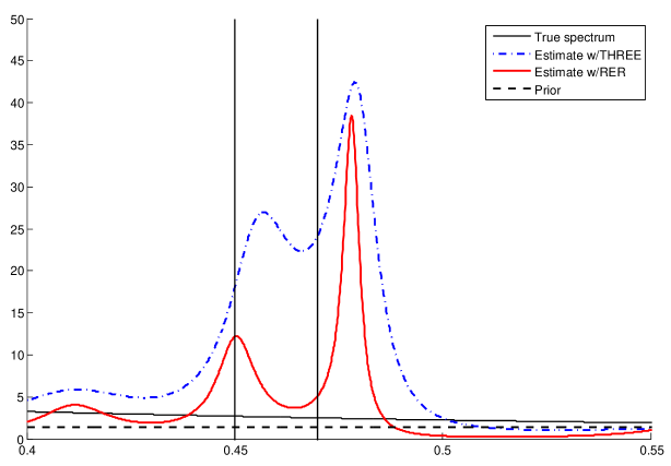
Figure 1: Estimation of close spectral lines in colored noise ($\omega_{1}=0.45$ rad/s and $\omega_{2}=0.47$ rad/s). The chosen prior is the sample covariance of the data $\{y_{k}\}$. The radius of the complex poles is equal to $0.95$. Both RER and THREE indicate the presence of the two lines.

In order to analyze such a feature, we deal with an instance of the classical problem of detecting spectral lines in colored noise. The setting is the same described in [5, Section IV.B]. The process of interest obeys to the following difference equation:

$$y(t)=0.5\sin(\omega_{1}t+\phi_{1})+0.5\sin(\omega_{2}t+\phi_{2})+z(t),\quad z(t)=0.8z(t-1)+0.5\nu(t)+0.25\nu(t-1),$$

where the variables $\phi_{1}$, $\phi_{2}$ and $\nu(t)$ are Gaussian, independent, with zero-mean and unit variance. Matrix $B$ is a column of ones. Matrix $A$ was chosen as a block-diagonal matrix; its real eigenvalues are $0$, $0.85$ and $-0.85$ and there are also five pairs of complex eigenvalues, whose arguments are equispaced in a narrow range of frequency where the sinusoids lie. Firstly, the spectral lines were fixed in $\omega_{1}=0.42$ rad/s and $\omega_{2}=0.53$ rad/s, and so the complex poles of $G(z)$ were chosen as:

$$0.9\rm{e}^{\pm j0.42},\,0.9\rm{e}^{\pm j0.44},\,0.9\rm{e}^{\pm j0.46},\,0.9\rm{e}^{\pm j0.48},\,0.9\rm{e}^{\pm j0.50}.$$

By considering the constant prior, equal to the sample covariance of the available data, the proposed method was able to detect both lines. We considered then the more challenging task when $\omega_{1}=0.45$ rad/s and $\omega_{2}=0.47$ rad/s. This choice makes the value of the distance between the two lines lower than the resolution limit of the periodogram, which amounts to $\frac{2\pi}{N}$ (which in our case is $\frac{2\pi}{300}\simeq 0.021$ rad/s). Nevertheless, choosing the poles closer to the unit circle, by fixing their radius to $0.95$, the RER estimator was still able to detect the presence of two lines. Figure 1 compares its performances with those achieved by THREE. In simulations, RER exhibited performances that were quite similar or slightly better than those of THREE, as in the case which is shown, where the peaks that were estimated are slightly closer to the real position of the spectral lines than those indicated by THREE. It was also observed that, in general, bringing the poles closer to the unit circle increases both the resolution and the variance of the estimates. The same trade-off was first described in [5] and seems to be typical of all THREE-like methods.

VII-B Multivariate Case

In order to test the performances of the proposed method in multivariate spectral estimation, we considered the same estimation task that is described in [42, Section VIII.C]. The process $y$ was obtained by filtering a bivariate Gaussian white noise process with zero mean and variance $I$ through a square shaping filter of order $40$. The filter coefficients were chosen at random, except for one fixed complex poles pair, $0.9\rm{e}^{\pm j0.52}$ and the zeros pair $(1-10^{-5})\rm{e}^{\pm j0.2}$.

We designed the filter $G(z)$ by fixing four complex poles pairs with radius $0.7$ and arguments equispaced in the range $\left[0,\pi\right]$. We assumed $N=300$ samples of the process $\{y_{k}\}_{k\in\mathbb{Z}}$ to be available. As for the the prior, our choice was to compute a simple PEM model of order $3$, by means of the standard function em␣␣rovided in Matlab. Figure 2 shows the real spectrum and the estimate computed by the RER approach.

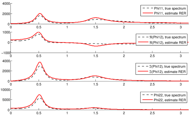
Figure 2: Multivariate spectrum estimation, $N=300$, PEM(3) prior. Comparison between the approximant and the true spectrum.

We then compared the performance of the proposed technique to those achieved by Maximum Entropy [20] and Hellinger-distance estimators, which are both THREE-like approaches to multivariate spectral estimation. Notice that the latter represented the state-of-the art of the convex optimization approach to spectral estimation in the multichannel framework [15]. In order to make the comparison as independent as possible of the specific data set, we performed $50$ trials by feeding the shaping filter with independent realizations of the input noise process. The criterion to evaluate the performances of each method was taken to be the average estimation error at each frequency, defined as

$$E_{M}(\vartheta):=\frac{1}{50}\sum_{i=1}^{50}\|\hat{\Phi}_{M}({\rm e}^{{{\rm j}}\vartheta})-\Phi({\rm e}^{{{\rm j}}\vartheta})\|.$$ (50)

Here M denotes the specific algorithm, $\hat{\Phi}_{M}$ is the corresponding approximant and the norm is the spectral norm (i.e. the largest singular value). Figure 3 allows to compare the various techniques. The results achieved by our approach are quite better than those of Maximum Entropy estimator (referred to as ME). Our RER method seems also to slightly outperform the Hellinger-distance approach. It is worth noticing that in the Hellinger case the order of the estimates was $19$, while in the case of RER it was just $11$. The order of the ME estimate is equal to $8$.

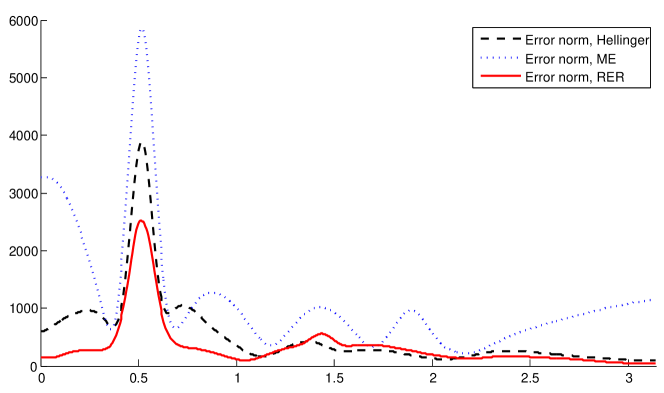
Figure 3: Comparison of THREE-like approaches in terms of average estimation error. $N=300$ available data. Both RER and Hellinger estimator are provided with a PEM(3) prior. All the considered methods make use of the same filter $G(z)$

It is interesting to investigate the case when only a few samples of the process $y$ are available. Shortness of the available data record, can heavily affect with artifacts the estimates obtained by classical methods such as Matlab’s PEM and N4SID. As the other THREE-like approaches, the RER method seems to be quite robust with respect to such a problem. Figure 4 shows the results obtained in a case where only $N=100$ samples are available. Both PEM and N4SID estimates are affected by artifacts. On the contrary, the proposed approach is not. This result seems to suggest that RER estimation is suitable to tackle spectral estimation issues characterized by the presence of short data records of the process of interest.

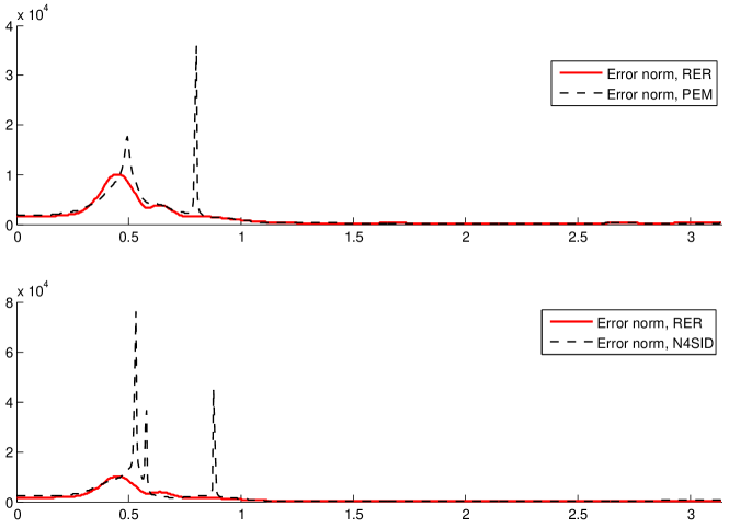
Figure 4: Comparison of Matlab’s PEM, Matlab’s N4SID and RER in terms of average estimation error. $N=100$ available samples. The prior considered for RER is a PEM(2) model. The filter $G(z)$ has a pole in the origin and four complex conjugate poles pairs with radius $0.7$. Notice that RER does not exhibit artifacts, whereas PEM and N4SID do.

VIII On the spectral representation of stationary Gaussian processes

We shall need the following result whose proof is given in the Appendix.

Lemma VIII.1

Let $u,v$ be $k$-dimensional, real random vectors with probability densities $p,q$, respectively. Let $f:\mathbb{R}^{k}\rightarrow\mathbb{R}^{h}$ be measurable and $p_{a},q_{a}$ be the probability densities of the augmented vectors $[u^{\top}\ f(u)^{\top}]^{\top}$ and $[v^{\top}\ f(v)^{\top}]^{\top}$, respectively. Then

$$\mbox{\BB D}(p_{a}\|q_{a})=\mbox{\BB D}(p\|q).$$ (51)

We also need to consider zero-mean, $n$-dimensional, complex-valued Gaussian random vectors $z=\alpha+j\beta$, where the real and imaginary parts are jointly Gaussian. The corresponding density function is the joint probability density of the $2n$-dimensional compound vector $\gamma=[\alpha^{\top}\beta^{\top}]^{\top}$. The differential entropy of the $n$-dimensional complex Gaussian density $p$ (defined exactly as in (1) but with integration taking place over $\mathbb{R}^{2n}$) with zero mean is given by

$$H(p)=-\int_{\mathbb{R}^{2n}}\log(p(x))p(x)dx=\frac{1}{2}\log(\det R)+\frac{1}{2}(2n)\left(1+\log(2\pi)\right),$$ (52)

where $R$ is the covariance matrix of the $2n$-dimensional vector $\gamma$. Similarly, the relative entropy between two zero-mean $n$-dimensional complex Gaussian densities $p$ and $q$ is given by

$$\mbox{\BB D}(p\|q):=\frac{1}{2}\left[\log\det(R_{p}^{-1}R_{q})+\mathop{\rm tr}(R_{q}^{-1}R_{p})-2n\right],$$ (53)

where $R_{p}$ and $R_{q}$ are the covariance matrices of the $2n$-dimensional vectors $\gamma_{p}$ and $\gamma_{q}$ corresponding to the densities $p$ and $q$, respectively. If the zero-mean, $\mathbb{C}^{n}$-valued Gaussian random vector $z$ has the property that $\mbox{\BB E}[zz^{\top}]=0$, then we say that $z$ is a circular symmetric normally distributed random vector [37]. This implies that $\mbox{\BB E}[\alpha\alpha^{T}]=\mbox{\BB E}[\beta\beta^{T}]$. If $p$ and $q$ are two $n$-dimensional complex Gaussian distribution with circular symmetry, the expression of the relative entropy simplifies to the formula

$$\mbox{\BB D}(p\|q)=\log\det(P^{-1}Q)+\mathop{\rm tr}(Q^{-1}P)-n,$$ (54)

where $P$ and $Q$ are the covariance matrices of $\gamma_{p}$ and $\gamma_{q}$, respectively.

We now state a few basic facts about the spectral representation of a stationary process that can be found, for instance, in [34, 45, 35]. Let $y=\{y_{k};\,k\in\mbox{\BB Z}\}$ be a $\mathbb{R}^{m}$-valued, zero-mean, Gaussian, stationary process and let $C_{l}:=E\{y_{k+l}y_{k}^{\top}\},\,l\in\mbox{\BB Z}$, be its covariance lags. Then

$$C_{l}=\frac{1}{2\pi}{\int_{-\pi}^{\pi}}e^{{{\rm j}}l\vartheta}{dF(\vartheta)},$$ (55)

where $F$ is a bounded, non-negative, matrix-valued measure called spectral measure. The stationary process $y$ admits itself the spectral representation

$$y_{k}={\int_{-\pi}^{\pi}}e^{{{\rm j}}k\vartheta}d\hat{y}(e^{{{\rm j}}\vartheta}),$$ (56)

where $\hat{y}$ is a $m$-dimensional stochastic orthogonal measure, see [45]. It may be obtained by defining, as in [35, pag. 44],

$$\chi_{k}(\vartheta_{1},\vartheta_{2}):=\begin{cases}\frac{e^{-{{\rm j}}\vartheta_{2}k}-e^{-{{\rm j}}\vartheta_{1}k}}{-2\pi{{\rm j}}k}&\text{if $k\neq 0$}\\ \frac{\vartheta_{2}-\vartheta_{1}}{2\pi}&\text{if $k=0$}\end{cases}\,,$$ (57)

and setting

$$\hat{y}(e^{{{\rm j}}\vartheta_{1}},e^{{{\rm j}}\vartheta_{2}}):=\lim_{N\rightarrow+\infty}\sum_{k=-N}^{N}\chi_{k}(\vartheta_{1},\vartheta_{2})y_{k}$$ (58)

where the sequence converges in mean square. We use the notation $d\hat{y}(e^{{{\rm j}}\vartheta})$ as a short-hand for $\hat{y}(e^{{{\rm j}}\vartheta},e^{{{\rm j}}(\vartheta+d\vartheta)})$ (with $d\vartheta>0$). It is well known that

$$\mbox{\BB E}\left\{d\hat{y}(e^{{{\rm j}}\vartheta})d\hat{y}(e^{{{\rm j}}\vartheta})^{*}\right\}=dF(\vartheta),$$ (59)

where $*$ denotes transposition plus conjugation. If the process $y$ is purely nondeterministic, then $dF(\vartheta)=\Phi_{y}(e^{{{\rm j}}\vartheta})d\vartheta$, where $\Phi_{y}$ is the spectral density function.

Proposition VIII.1

Suppose $\vartheta_{1},\vartheta_{2}\in(-\pi,\pi]$, then $\hat{y}(e^{-{{\rm j}}\vartheta_{2}},e^{-{{\rm j}}\vartheta_{1}})=\overline{\hat{y}(e^{{{\rm j}}\vartheta_{1}},e^{{{\rm j}}\vartheta_{2}})}$. If, moreover, $\vartheta_{1},\vartheta_{2}$ have the same sign, then, $\hat{y}(e^{{{\rm j}}\vartheta_{1}},e^{{{\rm j}}\vartheta_{2}})$ is a circularly symmetric, normally distributed random vector. Finally, let $\vartheta_{1},\vartheta_{2},\vartheta_{3},\vartheta_{4}$ be such that $[\vartheta_{1},\vartheta_{2}]\cap[\vartheta_{3},\vartheta_{4}]=[\vartheta_{1},\vartheta_{2}]\cap[-\vartheta_{4},-\vartheta_{3}]=\emptyset$. Then, $\hat{y}(e^{{{\rm j}}\vartheta_{1}},e^{{{\rm j}}\vartheta_{2}})$ and $\hat{y}(e^{{{\rm j}}\vartheta_{3}},e^{{{\rm j}}\vartheta_{4}})$ are independent random vectors.

Proof:

Observe that $\hat{y}(e^{{{\rm j}}\vartheta_{1}},e^{{{\rm j}}\vartheta_{2}})$ is a complex-valued random vector that may be written as $\hat{y}(e^{{{\rm j}}\vartheta_{1}},e^{{{\rm j}}\vartheta_{2}})=\hat{y}_{r}(e^{{{\rm j}}\vartheta_{1}},e^{{{\rm j}}\vartheta_{2}})+{\rm j}\hat{y}_{i}(e^{{{\rm j}}\vartheta_{1}},e^{{{\rm j}}\vartheta_{2}})$. In view of (58) the real part $\hat{y}_{r}(e^{{{\rm j}}\vartheta_{1}},e^{{{\rm j}}\vartheta_{2}})$ and the imaginary part $\hat{y}_{i}(e^{{{\rm j}}\vartheta_{1}},e^{{{\rm j}}\vartheta_{2}})$ are jointly Gaussian real random vectors, so $\hat{y}(e^{{{\rm j}}\vartheta_{1}},e^{{{\rm j}}\vartheta_{2}})$ is a complex-valued Gaussian vector. Since $y_{k}$ is a $\mathbb{R}^{m}$-valued process, $\hat{y}(e^{{{\rm j}}\vartheta_{1}},e^{{{\rm j}}\vartheta_{2}})$ (which may be thought of as an integrated version of a “Fourier transform”) has the Hermitian symmetry or equivalently $\hat{y}(e^{-{{\rm j}}\vartheta_{2}},e^{-{{\rm j}}\vartheta_{1}})=\overline{\hat{y}(e^{{{\rm j}}\vartheta_{1}},e^{{{\rm j}}\vartheta_{2}})}$. Moreover, for $\vartheta_{1}$ and $\vartheta_{2}$ with the same sign, $\hat{y}(e^{{{\rm j}}\vartheta_{1}},e^{{{\rm j}}\vartheta_{2}})$ and $\hat{y}(e^{-{{\rm j}}\vartheta_{2}},e^{-{{\rm j}}\vartheta_{1}})$ are orthogonal. Thus, we get

$$0=\mbox{\BB E}[\hat{y}(e^{{{\rm j}}\vartheta_{1}},e^{{{\rm j}}\vartheta_{2}})\hat{y}(e^{-{{\rm j}}\vartheta_{2}},e^{-{{\rm j}}\vartheta_{1}})^{*}]=\mbox{\BB E}[\hat{y}(e^{{{\rm j}}\vartheta_{1}},e^{{{\rm j}}\vartheta_{2}})\hat{y}(e^{{{\rm j}}\vartheta_{1}},e^{{{\rm j}}\vartheta_{2}})^{\top}]$$

or, equivalently, $\hat{y}(e^{{{\rm j}}\vartheta_{1}},e^{{{\rm j}}\vartheta_{2}})$ is circularly symmetric normally distributed. Finally, recall that two complex Gaussian random vectors $v_{1}$, $v_{2}$ are independent if and only if $E[v_{1}v_{2}^{\top}]=E[v_{1}v_{2}^{\ast}]=0$. In our case, by the orthogonality property, we have $E[\hat{y}(e^{{{\rm j}}\vartheta_{1}},e^{{{\rm j}}\vartheta_{2}})\hat{y}(e^{{{\rm j}}\vartheta_{3}},e^{{{\rm j}}\vartheta_{4}})^{\ast}]=0$ and $E[\hat{y}(e^{{{\rm j}}\vartheta_{1}},e^{{{\rm j}}\vartheta_{2}})\hat{y}(e^{{{\rm j}}\vartheta_{3}},e^{{{\rm j}}\vartheta_{4}})^{\top}]=E[\hat{y}(e^{{{\rm j}}\vartheta_{1}},e^{{{\rm j}}\vartheta_{2}})\hat{y}(e^{-{{\rm j}}\vartheta_{4}},e^{-{{\rm j}}\vartheta_{3}})^{\ast}]=0$.

 

IX Spectral relative entropy rate

Consider two zero-mean, jointly Gaussian, stationary, purely nondeterministic stochastic processes $y=\{y_{k};\,k\in\mbox{\BB Z}\}$ and $z=\{z_{k};\,k\in\mbox{\BB Z}\}$ taking values in $\mathbb{R}^{m}$ with spectral representation

$$y_{k}={\int_{-\pi}^{\pi}}e^{{\rm j}k\vartheta}d\hat{y}(e^{{{\rm j}}\vartheta}), \qquad\mbox{\BB E}\left\{d\hat{y}(e^{{{\rm j}}\vartheta})d\hat{y}(e^{{{\rm j}}\vartheta})^{*}\right\}=\Phi_{y}(e^{{{\rm j}}\vartheta})d\vartheta,$$ (60)

$$z_{k}={\int_{-\pi}^{\pi}}e^{{\rm j}k\vartheta}d\hat{z}(e^{{{\rm j}}\vartheta}), \qquad\mbox{\BB E}\left\{d\hat{z}(e^{{{\rm j}}\vartheta})d\hat{z}(e^{{{\rm j}}\vartheta})^{*}\right\}=\Phi_{z}(e^{{{\rm j}}\vartheta})d\vartheta.$$ (61)

Let $\vartheta_{k}=\frac{\pi k}{n}$, and consider the complex Gaussian random vectors $\delta\hat{y}_{k}:=\hat{y}(e^{{{\rm j}}\vartheta_{k}},e^{{{\rm j}}\vartheta_{k+1}})$ and $\delta\hat{z}_{k}:=\hat{z}(e^{{{\rm j}}\vartheta_{k}},e^{{{\rm j}}\vartheta_{k+1}})$, with $k=0,1\dots,2n$. Define now the random vectors

$$\hat{Y}_{k}:=\begin{bmatrix}\delta\hat{y}_{0}\\ \vdots\\ \delta\hat{y}_{k-1}\end{bmatrix},\quad\hat{Z}_{k}:=\begin{bmatrix}\delta\hat{z}_{0}\\ \vdots\\ \delta\hat{z}_{k-1}\end{bmatrix},\quad k=1,\dots,2n,$$ (62)

and denote their joint probability density by $p(\hat{Y}_{k})$ and $p(\hat{Z}_{k})$, respectively.

Definition IX.1

The spectral relative entropy rate between between $y$ and $z$ is defined by the following limit, provided it exists:

$${{\mbox{\BB D}_{r}(d\hat{y}\|d\hat{z})}:=}\lim_{n\rightarrow\infty}\frac{1}{2n}\mbox{\BB D}\left(p(\hat{Y}_{2n})\|p(\hat{Z}_{2n})\right).$$ (63)

We now establish a remarkable connection between time-domain and spectral-domain relative entropy rates.

Theorem IX.1

Let $y$ and $z$ be as above. Assume that both $\Phi_{y}$ and $\Phi_{z}$ are piecewise continuous, coercive spectral densities. The following equality holds:

$$\mbox{\BB D}_{r}(y\|z)=\mbox{\BB D}_{r}(d\hat{y}\|d\hat{z}).$$ (64)

Proof:

In view of Proposition VIII.1, the last $n$ components of $\hat{Y}_{2n}$ are functions (the complex conjugate) of the first $n$ and the same holds for $\hat{Z}_{2n}$. Hence, in view of Lemma VIII.1, we have $\mbox{\BB D}\left(p(\hat{Y}_{2n})\|p(\hat{Z}_{2n})\right)=\mbox{\BB D}\left(p(\hat{Y}_{n})\|p(\hat{Z}_{n})\right)$. Using again Proposition VIII.1, we have that the elements of $\hat{Y}_{n}$ are independent random vectors and the same holds for the elements of $\hat{Z}_{n}$. Hence, we have the following additive decomposition:

$$\mbox{\BB D}\left(p(\hat{Y}_{2n})\|p(\hat{Z}_{2n})\right)=\mbox{\BB D}\left(p(\hat{Y}_{n})\|p(\hat{Z}_{n})\right)=\sum_{k=0}^{n-1}\mathbb{D}\left(p(\delta\hat{y}_{k})\|p(\delta\hat{z}_{k})\right),$$ (65)

with $p(\delta\hat{y}_{k})$ and $p(\delta\hat{z}_{k})$ being the probability densities of the random vector ${\delta\hat{y}_{k}}=\hat{y}(e^{{\rm j}\vartheta_{k}},e^{{\rm j}\vartheta_{k+1}})$ and ${\delta\hat{z}_{k}=}\hat{z}(e^{{\rm j}\vartheta_{k}},e^{{\rm j}\vartheta_{k+1}})$, respectively. Since $\delta\hat{y}_{k}$ and $\delta\hat{z}_{k}$ are jointly Gaussian and circularly symmetric, by (54) and (60)-(61), we get,

$$\mbox{\BB D}\left(p(\delta\hat{y}_{k})\|p(\delta\hat{z}_{k})\right)=\log\det\left[Q_{y}^{-1}(\vartheta_{k},\vartheta_{k+1})Q_{z}(\vartheta_{k},\vartheta_{k+1})\right]\\ +\mathop{\rm tr}\left[Q_{z}^{-1}(\vartheta_{k},\vartheta_{k+1})Q_{y}(\vartheta_{k},\vartheta_{k+1})\right]-m,$$ (66)

where, by virtue of the orthogonal increments property,

$$Q_{y}(\vartheta_{k},\vartheta_{k+1}):=\int_{\vartheta_{k}}^{\vartheta_{k+1}}\Phi_{y}(e^{{{\rm j}}\xi})d\xi,\qquad Q_{z}(\vartheta_{k},\vartheta_{k+1}):=\int_{\vartheta_{k}}^{\vartheta_{k+1}}\Phi_{z}(e^{{{\rm j}}\xi})d\xi.$$ (67)

By piecewise continuity and the mean value theorem, we have that, except for a finite number of $k$’s,

$$\begin{split}\mbox{\BB D}\left(p(\delta\hat{y}_{k})\|p(\delta\hat{z}_{k})\right)&=\log\det\left[\left(\Phi_{y}(e^{{{\rm j}}{\bar{\vartheta}_{k}}})\frac{\pi}{n}\right)^{-1}\Phi_{z}(e^{{{\rm j}}{\bar{\vartheta}_{k}}})\frac{\pi}{n}\right]+\mathop{\rm tr}\left[\left(\Phi_{z}(e^{{{\rm j}}{\bar{\vartheta}_{k}}})\frac{\pi}{n}\right)^{-1}\Phi_{y}(e^{{{\rm j}}{\bar{\vartheta}_{k}}})\frac{\pi}{n}\right]-m\\ &=\log\det[\Phi_{y}(e^{{{\rm j}}{\bar{\vartheta}_{k}}})^{-1}\Phi_{z}(e^{{{\rm j}}{\bar{\vartheta}_{k}}})]+\mathop{\rm tr}\left[\Phi_{z}(e^{{{\rm j}}{\bar{\vartheta}_{k}}})^{-1}\Phi_{y}(e^{{{\rm j}}{\bar{\vartheta}_{k}}})\right]-m,\end{split}$$ (68)

where $\vartheta_{k}\leq\bar{\vartheta}_{k}<\vartheta_{k+1}$. By employing the latter expression together with (65) and (63), we get

$$\begin{split}\mbox{\BB D}_{r}(d\hat{y}\|d\hat{z})&=\lim_{n\rightarrow\infty}\frac{1}{2n}\mathbb{D}\left(\hat{Y}_{n}\|\hat{Z}_{n}\right)=\lim_{n\rightarrow\infty}\frac{1}{2n}\sum_{k=0}^{n-1}\mbox{\BB D}\left(p(\delta\hat{y}_{k})\|p(\delta\hat{z}_{k})\right)\\ &=\lim_{n\rightarrow\infty}\frac{1}{2n}\sum_{k=0}^{n-1}\log\det\Phi_{y}(e^{{{\rm j}}{\bar{\vartheta}_{k}}})^{-1}\Phi_{z}(e^{{{\rm j}}{\bar{\vartheta}_{k}}})+\mathop{\rm tr}\left[\Phi_{z}^{-1}(e^{{{\rm j}}{\bar{\vartheta}_{k}}})\left(\Phi_{y}(e^{{{\rm j}}{\bar{\vartheta}_{k}}})-\Phi_{z}(e^{{{\rm j}}{\bar{\vartheta}_{k}}})\right)\right]\\ &=\lim_{n\rightarrow\infty}\frac{1}{2\pi}\sum_{k=0}^{n-1}\left\{\log\det\Phi_{y}(e^{{{\rm j}}{\bar{\vartheta}_{k}}})^{-1}\Phi_{z}(e^{{{\rm j}}{\bar{\vartheta}_{k}}})+\mathop{\rm tr}\left[\Phi_{z}^{-1}(e^{{{\rm j}}{\bar{\vartheta}_{k}}})\left(\Phi_{y}(e^{{{\rm j}}{\bar{\vartheta}_{k}}})-\Phi_{z}(e^{{{\rm j}}{\bar{\vartheta}_{k}}})\right)\right]\right\}\frac{\pi}{n}\\ &=\frac{1}{2\pi}\int_{0}^{\pi}\left\{\log\det\left(\Phi_{y}^{-1}(e^{{{\rm j}}\vartheta})\Phi_{z}(e^{{{\rm j}}\vartheta})\right)+\mathop{\rm tr}\left[\Phi_{z}^{-1}(e^{{{\rm j}}\vartheta})\left(\Phi_{y}(e^{{{\rm j}}\vartheta})-\Phi_{z}(e^{{{\rm j}}\vartheta})\right)\right]\right\}d\vartheta\\ &=\frac{1}{4\pi}{\int_{-\pi}^{\pi}}\left\{\log\det\left(\Phi_{y}^{-1}(e^{{{\rm j}}\vartheta})\Phi_{z}(e^{{{\rm j}}\vartheta})\right)+\mathop{\rm tr}\left[\Phi_{z}^{-1}(e^{{{\rm j}}\vartheta})\left(\Phi_{y}(e^{{{\rm j}}\vartheta})-\Phi_{z}(e^{{{\rm j}}\vartheta})\right)\right]\right\}d\vartheta,\end{split}$$

which, by (9), is (64).  

Remark IX.1

As is well known, the fundamental property of the Fourier transform is that it is isometric. The above result may be interpreted as a further invariance principle of the Fourier transform: the relative entropy rate is the same in the time and spectral domain.

X Conclusion

In this paper, a profound information-theoretic result relating time and spectral domain relative entropy rates of stationary Gaussian processes has been established. Motivated by this result, a new THREE-like approach to multivariate spectral estimation, called RER, has been introduced and tested. It appears as the most natural extension of maximum entropy methods when a prior estimate of the spectrum is available. It features an upper bound on the complexity of the estimate which is equal to the one provided by THREE in the scalar context, sensibly improving on the best one so far available in the multichannel setting with prior estimate. As for previous THREE-like methods, RER exhibits high resolution features and works extremely well with short observation records outperforming Matlab’s PEM and Matlab’s N4SID.

References

• [1] M. Basseville. Distance Measures for Signal Processing and Pattern Recognition. Signal Processing, 18:349–369, 1989.
• [2] A. Blomqvist, A. Lindquist, and R. Nagamune. Matrix-valued Nevanlinna-Pick interpolation with complexity constraint: An optimization approach. IEEE Trans. Aut. Control, 48:2172–2190, 2003.
• [3] S. Boyd and L. Vandenberghe. Convex Optimization. Cambridge University Press, Cambridge, UK, 2004.
• [4] C. I. Byrnes, P. Enqvist, and A. Linquist. Identifiability and well-posedness of shaping-filter parameterizations: A global analysis approach. SIAM J. Control and Optimization, 41:23–59, 2002.
• [5] C. I. Byrnes, T. Georgiou, and A. Lindquist. A new approach to spectral estimation: A tunable high-resolution spectral estimator. IEEE Trans. Sig. Proc., 48:3189–3205, 2000.
• [6] C. I. Byrnes, T. Georgiou, and A. Lindquist. A generalized entropy criterion for Nevanlinna-Pick interpolation with degree constraint: A convex optimization approach to certain problems in systems and control. IEEE Trans. Aut. Control, 46:822–839, 2001.
• [7] C. I. Byrnes, T. Georgiou, A. Lindquist, and A. Megretski. Generalized interpolation in H-infinity with a complexity constraint. Trans. American Math. Society, 358(3):965–987, 2006.
• [8] C. I. Byrnes, S. Gusev, and A. Lindquist. A convex optimization approach to the rational covariance extension problem. SIAM J. Control and Opimization, 37:211–229, 1999.
• [9] C. I. Byrnes and A. Linquist. Important moments in systems and control. SIAM J. Contr. Opt., 47(5):2458–2469, 2008.
• [10] C.I. Byrnes and A. Lindquist. On the partial stochastic realization problem. IEEE Trans. Aut. Contr., 42:1049–1070, 1997.
• [11] C.I. Byrnes, A. Lindquist, S. Gusev, and A. S. Matveev. A complete parameterization of all positive rational extensions of a covariance sequence. IEEE Trans. Aut. Contr., 40:1841–1857, 1995.
• [12] T. M. Cover and J. A. Thomas. Information Theory. Wiley, New York, 1991.
• [13] A. Dembo and O. Stroock. Large Deviation Techniques and Applications. Jones and Bartlett Publishers, 1993.
• [14] P. Enqvist and J. Karlsson. Minimal itakura-saito distance and covariance interpolation. In 47th IEEE Conference on Decision and Control, CDC 2008., pages 137 –142, 9-11 2008.
• [15] A. Ferrante, M. Pavon, and F. Ramponi. Hellinger vs. Kullback-Leibler multivariable spectrum approximation. IEEE Trans. Aut. Control, 53:954–967, 2008.
• [16] A. Ferrante, M. Pavon, and M. Zorzi. A maximum entropy enhancement for a family of high-resolution spectral estimators. IEEE Trans. Aut. Control, June 2010 (to appear).
• [17] T. Georgiou. Realization of power spectra from partial covariance sequences. IEEE Trans. on Acoustics, Speech, and Signal Processing, 35:438–449, 1987.
• [18] T. Georgiou. The interpolation problem with a degree constraint. IEEE Trans. Aut. Control, 44:631–635, 1999.
• [19] T. Georgiou. Spectral estimation by selective harmonic amplification. IEEE Trans. Aut. Control, 46:29–42, 2001.
• [20] T. Georgiou. Spectral analysis based on the state covariance: the maximum entropy spectrum and linear fractional parameterization. IEEE Trans. Aut. Control, 47:1811–1823, 2002.
• [21] T. Georgiou. The structure of state covariances and its relation to the power spectrum of the input. IEEE Trans. Aut. Control, 47:1056–1066, 2002.
• [22] T. Georgiou. Solution of the general moment problem via a one-parameter imbedding. IEEE Trans. Aut. Control, 50:811–826, 2005.
• [23] T. Georgiou. Distances between power spectral densities. IEEE Trans. Aut. Control, 47:1056–1066, 2006.
• [24] T. Georgiou. Relative entropy and the multivariable multidimensional moment problem. IEEE Trans. Inform. Theory, 52:1052–1066, 2006.
• [25] T. Georgiou. The Meaning of Distance in Spectral Analysis. In 46th IEEE Conference on Decision and Control, New Orleans, U.S.A., pages http://www.ieeecss–oll.org/video/meaning–distances–spectral–analysis, Dec. 12 2007.
• [26] T. Georgiou. Distances and Riemannian Metrics for Spectral Density Functions. IEEE Trans. on Signal Processing, 55(8):3995–4003, August 2007.
• [27] T. Georgiou and A. Lindquist. Kullback-Leibler approximation of spectral density functions. IEEE Trans. Inform. Theory, 49:2910–2917, 2003.
• [28] T. Georgiou and A. Lindquist. Remarks on control design with degree constraint. IEEE Trans. Aut. Control, AC-51:1150–1156, 2006.
• [29] T. Georgiou and A. Lindquist. A convex optimization approach to ARMA modeling. IEEE Trans. Aut. Control, AC-53:1108–1119, 2008.
• [30] R. Gray, A. Buzo, A. Jr Gray, and Y. Matsuyama. Distortion measures for speech processing. IEEE Trans. Acoustics, Speech and Signal Proc., 28:367–376, 1980.
• [31] S. Ihara. Information Theory for Continuous Systems. World Scientific, Singapore, 1993.
• [32] X. Jiang, L. Ning, and T. Georgiou. Distances and riemannian metrics for multivariate spectral densities. preprint, June 2011.
• [33] A.N. Kolmogorov. On the Shannon theory of information in the case of continuous signals. IRE Trans. Inform. Theory, 2:102–108, 1956.
• [34] H. Kramer and M. R. Leadbetter. Stationary and Related Stochastic Processes. Wiley, New York, 1966.
• [35] A. Lindquist and G. Picci. Linear Stochastic Systems: A Geometric Approach to Modeling, Estimation and Identification. In preparation: preprint available in http://www.math.kth.se/~alq/LPbook.
• [36] J. H. McClellan. Multidimensional spectral estimation. Proc. IEEE, 70:1029–1039, 1982.
• [37] K. S. Miller. Complex Stochastic Processes. Addison Wesley, Reading, MA, 1974.
• [38] A. Nasiri Amini, E. Ebbini, and T. Georgiou. Noninvasive estimation of tissue temperature via high-resolution spectral analysis techniques. IEEE Trans. on Biomedical Engineering, 52:221–228, 2005.
• [39] M. A. Nielsen and I. L. Chuang. Quantum Computation and Quantum Information. Cambridge Univ. Press, 2000.
• [40] M. S. Pinsker. Information and information stability of random variables and processes. Holden-Day, San Francisco, 1964. Translated by A. Feinstein.
• [41] P. Dai Pra. Private communication. June 2011.
• [42] F. Ramponi, A. Ferrante, and M. Pavon. A globally convergent matricial algorithm for multivariate spectral estimation. IEEE Transactions on Automatic Control, 54(10):2376–2388, Oct. 2009.
• [43] R. T. Rockafellar. Convex Analysis. Princeton University Press, Princeton, NJ, 1970.
• [44] O. Rosen and D. Stoffer. Automatic estimation of multiv. spectra via smoothing splines. Biometrika, 94:335–345, 2007.
• [45] Yu. A. Rozanov. Stationary Random Processes. Holden-Day, San Francisco, 1967.
• [46] P. Stoica and R. Moses. Introduction to Spectral Analysis. Prentice Hall, New York, 1997.
• [47] A. A. Stoorvogel and J. H. Van Schuppen. System identification with information theoretic criteria. In S. Bittanti and G. Picci, editors, Identification, Adaptation, Learning: The Science of Learning Models from Data. Springer, 1996.
• [48] A. Van Den Bos. The Multivariate Complex Normal Distribution - A Generalization. IEEE Trans. Inform. Theory, 41:537–539, 1995.