Non-linear interaction in random matrix models of RNA

Abstract

A non-linear Penner type interaction is introduced and studied in the random matrix model of homo-RNA. The asymptotics in length of the partition function is discussed for small and large $N$ (size of matrix). The interaction doubles the coupling ($v$) between the bases and the dependence of the combinatoric factor on ($v,N$) is found. For small $N$, the effect of interaction changes the power law exponents for the secondary and tertiary structures. The specific heat shows different analytical behavior in the two regions of $N$, with a peculiar double peak in its second derivative for $N=1$ at low temperature. Tapping the model indicates the presence of multiple solutions.

In the fundamental understanding of RNA folding combinatorics, the study of exact enumeration of RNA secondary structures with crossings (pseudoknots) is an important ongoing research direction 1 . In this context, Orland and Zee proposed a random matrix-field theoretic model 2 which addressed the problem of exact RNA structure combinatorics which with certain simplifying assumptions 3 enumerated all possible planar and non-planar structures. In this model, the idea of introducing external linear interaction was explored in 4 ; 5 ; 6 with the objective to observe structural and other statistical changes (if any). Even with this simple interaction, it was shown that the interaction imposed additional constraints on the RNA chain which could physically imply changes in temperature, applied pressure, proximity with ions 6 . So, within this matrix model framework, an important interaction to study is the Penner type that may capture interesting properties such as: effects of interactions with more complex molecules and biomolecules, multiple solutions, frozen (glassy) states 7 . The Penner matrix models appear in the context of disordered systems 8 (initially to calculate correct fluctuations for the conductance), string theory 9 (to get accurate critical exponents for quantum gravity) and spin glasses 10 (as mappings to high temperature $p$-spin glasses). In this letter studying the Penner type interactions increases the moduli space of structures from ${\cal M}_{g,0}$ to ${\cal M}_{g,n}$ where $g$ is the genus of the surface and $n$ gives the number of faces or punctures of the Riemann surfaces. Thus the generalized partition function of RNA matrix model (of length $L$: $(i,j)=1,....,L$) with a logarithmic interaction in the action is given by

$$Z_{L}(N)=\frac{1}{A_{L}(N)}\int\prod_{i=1}^{L}d\phi_{i}e^{-\frac{N}{2}\sum_{i,j=1}^{L}(V^{-1})_{i,j}Tr\phi_{i}\phi_{j}}e^{\frac{N}{2}\sum_{i=1}^{L}(W^{-1})_{i}Tr[\log\phi_{i}^{2}]}\frac{1}{N}Tr\prod_{i=1}^{L}(1+\phi_{i}),$$ (1)

where $\phi_{i}$’s are $L$ independent ($N\times N$) random (symmetric) hermitian matrices placed at each base site in the chain with the interactions contained in $V_{ij}$ (see 2 ; 3 ; 4 for all other notations and conventions). The normalization constant is given by

$$A_{L}(N)=\int\prod_{i=1}^{L}d\phi_{i}e^{-\frac{N}{2}\sum_{i,j=1}^{L}(V^{-1})_{i,j}Tr\phi_{i}\phi_{j}}e^{\frac{N}{2}\sum_{i=1}^{L}(W^{-1})_{i}Tr[\log\phi_{i}^{2}]},$$ (2)

and $\frac{1}{N}Tr\prod_{i}(1+\phi_{i})$ is the characteristic observable of the model. With the simplifications, $V_{ij}=v$ and $W_{i}=w$, and a series of Hubbard Stratonovich Transformations 4 , Eq. (1) becomes

$$Z_{L}(N)=\frac{1}{A^{\prime}_{L}(N)}\int d\sigma e^{-NTr[\frac{1}{2v}\sigma^{2}-\frac{1}{2w}(\log\sigma^{2})]}\frac{1}{N}Tr(1+\sigma)^{L},$$ (3)

where $\sigma$ is an ($N\times N$) matrix, the potential is given by $V(\sigma)=[\frac{\mu}{2}\sigma^{2}-\frac{t^{\prime\prime}}{2}\log\sigma^{2}]$ (with $\mu=1/v$, $t^{\prime\prime}=1/w$) and the normalization is

$$A^{\prime}_{L}(N)=\int d\sigma e^{-NTr[\frac{1}{2v}\sigma^{2}-\frac{1}{2w}\log\sigma^{2}]}.$$ (4)

These potentials are of the Gaussian Penner matrix models 9 and will be solved along those lines. The spectral density $\rho_{N}(z)$ of the matrix $\sigma$ at finite $N$ is

$$\rho_{N}(z)=\frac{1}{A^{\prime}_{L}(N)}\int d\sigma e^{-NTrV(\sigma)}\frac{1}{N}Tr\delta(z-\sigma),$$ (5)

where $z$ are the eigenvalues of $\sigma$. Defining $G(t,N)=\sum_{L=0}^{\infty}Z_{L}(N)\frac{t^{L}}{L!}$ as the exponential generating function of the partition function 3 ; 4 and using the identity $\int_{-\infty}^{+\infty}dz\rho_{N}(z)=1$ gives

$$G(t,N)=\int_{-\infty}^{+\infty}dz\rho_{N}(z)exp^{t(1+z)}.$$ (6)

To solve $G(t,N)$, the expression for spectral density is found using the orthogonal polynomial method (Deo, 9 ). For these models, the orthogonal polynomials are given by ${\cal P}_{n}(z)=z^{n}+l.o.$ which satisfy the orthogonality condition,

$$\int_{-\infty}^{+\infty}dze^{-NV(z)}{\cal P}_{n}(z){\cal P}_{m}(z)=h_{n}\delta_{nm}.$$ (7)

For the symmetric Gaussian Penner matrix model, orthogonal polynomials split into even and odd polynomials. The even set obeys the orthogonality condition

$$\int_{0}^{\infty}dye^{-N^{\prime}[\nu_{0}(y)-t^{\prime}\log y]}{\cal P}_{n}(y){\cal P}_{m}(y)=h_{n}\delta_{nm},$$ (8)

where $y=z^{2}$, $N^{\prime}=N/2$, $\nu_{0}(y)=2V_{0}(z)=\mu y+....$ and $t^{\prime}=(t^{\prime\prime}-\frac{1}{2N^{\prime}})$. The odd ones obey

$$\int_{0}^{\infty}dye^{-N^{\prime}[\nu_{0}y-{\bar{t}}^{\prime}\log y]}{\bar{\cal P}}_{n}(y){\bar{\cal P}}_{m}(y)={\bar{h}}_{n}\delta_{nm},$$ (9)

where ${\bar{t}}^{\prime}=(t^{\prime\prime}+\frac{1}{2N^{\prime}})$. It is sufficient to work with either of the two polynomials as each one can completely determine the recursion coefficients independent of the other. The normalized even orthogonal polynomials from solving the orthogonality relations are

$$\psi_{2n}(y)=e^{-\frac{N^{\prime}}{2}[\mu y-t^{\prime}\log y]}\hat{{\cal P}}_{n}(y)=\left[\frac{n!(N^{\prime}\mu)^{N^{\prime}t^{\prime}+1}}{\Gamma(n+1+N^{\prime}t^{\prime})}\right]^{1/2}y^{\frac{N^{\prime}t^{\prime}}{2}}e^{-\frac{N^{\prime}\mu y}{2}}L^{N^{\prime}t^{\prime}}_{n}(N^{\prime}\mu y),$$ (10)

which in the case of odd polynomials has ${\bar{t}}^{\prime}$ instead of $t^{\prime}$. The kernel for this function is defined by $K(y_{i},y_{j})=\sum_{n=0}^{N-1}\psi_{2n}(y_{i})\psi_{2n}(y_{j})$ which gives the normalized spectral density for the even polynomials as $\rho^{e}_{N}(y)=\frac{1}{N}K(y,y)$ (the superscript $e$ represents even). Thus the spectral density for large $N$ limit is

$$\rho^{e}_{N}(z^{2})=\frac{1}{N}\sum_{n=0}^{N-1}\left[\frac{n!(N^{\prime}\mu)^{N^{\prime}t^{\prime}+1}}{\Gamma(n+1+N^{\prime}t^{\prime})}\right]z^{2N^{\prime}t^{\prime}}e^{-N^{\prime}\mu z^{2}}[L^{N^{\prime}t^{\prime}}_{n}(N^{\prime}\mu z^{2})]^{2},$$ (11)

where $y=z^{2}$ is considered. Using the relation $\rho^{e}_{N}(z)=z\rho^{e}_{N}(z^{2})$ (Tan; Deo in 9 ) and substituting $\rho^{e}_{N}(z^{2})$ in the generating function for the even polynomials, Eq. (6) gives

Table 1: The Table lists even partition functions for $L$ upto 6 for the matrix model with logarithmic interaction.

$L$	$Z^{e}_{L}(N)$
1	1
2	$1+v(2+\frac{1}{N})$
3	$1+3v(2+\frac{1}{N})$
4	$1+6v(2+\frac{1}{N})+2v^{2}(4+\frac{3}{N})+\frac{v^{2}}{N^{2}}$
5	$1+10v(2+\frac{1}{N})+10v^{2}(4+\frac{3}{N})+\frac{5v^{2}}{N^{2}}$
6	$1+15v(2+\frac{1}{N})+30v^{2}(4+\frac{3}{N})+5v^{3}(8+\frac{8}{N}+\frac{1}{N^{3}})$
	$+(15v^{2}+20v^{3})/N^{2}$

$$G^{e}(t,N)=\frac{1}{N}\sum_{n=0}^{N-1}\left[\frac{n!(N^{\prime}\mu)^{N^{\prime}t^{\prime}+1}}{\Gamma(n+1+N^{\prime}t^{\prime})}\right]e^{\frac{t^{2}}{4N^{\prime}\mu}+t}\int_{-\infty}^{+\infty}\frac{dx}{\sqrt{N^{\prime}\mu}}\left[\frac{x}{\sqrt{N^{\prime}\mu}}\right]^{2N^{\prime}t^{\prime}+1}e^{-\left[x-\frac{t}{2\sqrt{N^{\prime}\mu}}\right]^{2}}\left[L^{N^{\prime}t^{\prime}}_{n}(x^{2})\right]^{2}.$$ (12)

To solve this integral, a simplification is made, $N^{\prime}t^{\prime}=1/2$ ($-1/2$ for the odd) which requires $t^{\prime\prime}=2/N$ ($-2/N$ for the odd). Substituting this and using the relation $H_{2n+1}(x)=(-1)^{n}2^{2n+1}n!xL^{1/2}_{n}(x^{2})$ (for odd polynomials, $H_{2n}(x)=(-1)^{n}2^{2n}n!L^{-1/2}_{n}(x^{2})$) in Eq. (12) gives

$$G^{e}(t,N)=\frac{1}{N}\sum_{n=0}^{N-1}\left[\frac{e^{\frac{t^{2}}{4N^{\prime}\mu}+t}}{\Gamma(n+\frac{3}{2})}\right]\frac{1}{n!(2^{2n+1})^{2}}\int_{-\infty}^{+\infty}dxe^{-\left[x-\frac{t}{2\sqrt{N^{\prime}\mu}}\right]^{2}}\\ \times\left[H_{2n+1}(x)\right]^{2}.$$ (13)

Using the formula $[H_{k}(x)]^{2}=\sum_{l=0}^{k}\frac{(k!)^{2}2^{k-l}}{(l!)^{2}(k-l)!}H_{2l}(x)$ and the integral $\int_{-\infty}^{+\infty}dxe^{-(x-y)^{2}}H_{n}(x)=\sqrt{\Pi}y^{n}2^{n}$, $G^{e}(t,N)$ becomes

$$G^{e}(t,N)=\frac{1}{N}e^{\frac{t^{2}}{4N^{\prime}\mu}+t}\sum_{n=0}^{N-1}\sum_{l=0}^{2n+1}\binom{2n+1}{l}\frac{t^{2l}}{l!(2N^{\prime}\mu)^{l}},$$ (14)

which differs from odd polynomials in $\sum_{l=0}^{2n}\binom{2n}{l}$. The partition functions can be obtained from Eq. (13) (Table I). The general form of the partition function for any $N^{\prime}t^{\prime}$ requires a rigorous mathematical analysis and is left for a future work. In this model, $N$ plays a dual role of contributing to the strength of the external interaction and a genus identification parameter of the structures. However with $N^{\prime}t^{\prime}=(1/2,-1/2)$, the genus characterization cannot be extracted systematically. In the model of 2 ; 3 , the structures (and their genus characterization) were obtained on the moduli space of a zero puncture Riemann surface ${\cal M}_{g,0}$. Constructing the matrix model of RNA with a logarithmic interaction generalizes the study of RNA structures to that of $n$-punctured Riemann surfaces, ${\cal M}_{g,n}$. The Euler characteristics for these models are given by $(V-E+n)=(2-2g)$ where $V$ and $E$ give the number of vertices and edges respectively and includes the additional factor of faces or punctures $n$. The genus characterization of the structures obtained from the model is therefore changed from 3 . For this model the Feynman diagrams are given by the fat-graphs 9 .

I Asymptotic Analysis of the partition function

The asymptotic behavior of the partition function at large length is found numerically as in 5 . The analysis is divided into two parts, (I) the estimation of structure combinatoric factor and (II) the determination of (secondary and tertiary) power law exponents with $L$.

I.1 Combinatorics

The combinatorics of the structures is given by $X=(2\sqrt{f(v,N)}+1)^{L}$ where (i) $X=3^{L}$ for the model in 3 and (ii) $X=(3-\alpha)^{L}$ in 5 (here $f(v,N)=v=1$ in both the cases). The analysis is done for lengths upto $L=(40,80,160)$. For each length, different $v$ $(1$ to $6)$ are considered and for each $v$ different values of $N$ (1 to 100000) are chosen so as to observe the effect of interaction. In order to determine the form of $f(v,N)$ for this model, $ln[Z^{e}_{L}(N)]$ is plotted with $L$ for different $(L,v,N)$. The linearly fitted slopes and intercepts are found. For a given $v$,
(i) $f(v,N)$’s for each $N$ are found from the slopes using the expression $f(v,N)=(\frac{e^{Slope}-1}{2})^{2}$ and
(ii) $f(v,N)$’s hence found are plotted linearly with $1/N$.

Therefore for each $v$, a functional form of $f(v,N)$ is obtained in terms of $1/N$. Then for each length, the slopes and intercepts from the functional forms of $f(v,N)$ for different $v$ are plotted as a function of $v$ to obtain the final $f_{L}(v,N)$ expression. For the log interaction the form is found to be $f^{log}(v,N)=\left[2v_{oz}(1+\frac{a_{oz}}{2N})\right]$ where $a_{oz}\sim 16$ for $L=160$ and for the $oz$ model it is $f^{oz}(v,N)=\left[v_{oz}(1+\frac{a_{oz}}{N})\right]$. This results in two observations: (i). The base pairing interaction strength $v_{oz}$ in 3 is doubled. This implies, $v$ in the log interaction model is re-scaled to twice the $v$ in the $oz$ model which is similar to the way in which the parameter $\alpha$ in the linear interaction model 6 re-scaled $v$ to $v/(1-\alpha)^{2}$. (ii). An additional dependence of the combinatoric factor on $N$ is found ($va/N$) for all small and large values of $N$ for the log interaction and $oz$ models (which comes out to be same). Such a dependence has not been found before in these matrix models.

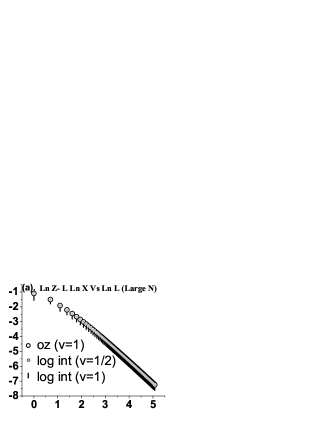
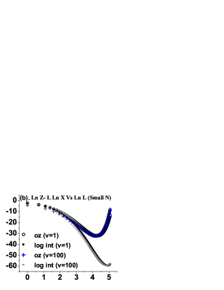
Figure 1: $LnZ^{e}_{L}(N)-LlnX$ is plotted with $lnL$ for the log interaction and $oz$ models for (a). $N=1000000$ and (b). $N=1$.

I.2 Power law exponents

In order to extract the exponents corresponding to secondary and tertiary contributions, the $lnL$ dependence in the partition function is studied. This analysis is done for $L=160$ and is divided into small $N$ ($N=1$) and large $N$ ($N=100000$) regions.

I.2.1 Large $N$

To study the secondary exponent, ($lnZ-LlnX$) is plotted with $lnL$ (Fig1(a)). (i) The plot is a straight line with slope $-1.37$ which approaches $-1.5$ when larger and larger values of $N$ are considered. This implies at large $N$, the major contribution is from the genus zero (secondary) structures and the power law $L^{-3/2}$ holds true as for the $oz$ and linear interaction models 3 ; 4 ; 5 ; 6 . (ii) For $v=1$, the $oz$ and log interaction curves are distinctly different. On substituting $v=1/2$ in the log partition function, the two model curves coincide. So for large $N$ and $v=1/2$, the structures in the log interaction model reduce exactly to the structures found in the $oz$ model. Thus the effect of interaction at large $N$ is visible in terms of $v$ only. (iii) The slopes of the curves for different $v$’s are nearly $-1.37$ implying that the slope (i.e. the exponent $-3/2$) is independent of $v$. (b). Next, to study the tertiary exponent, ($lnZ-LlnX+(3/2)lnL$) is plotted with $L$ which shows: (i) the structure of the curves for the two models is exactly the same. So the genus contribution in the large $N$ limit has the same form for both the models. (ii) The extrapolation of curves on y axis gives the value of $k_{0}$ (for large $N$, see 3 ). For $v=1$, these are different for the two models showing that the coefficients $k_{g}$’s will be different. For large values of $v$, the points for the even and odd lengths (at small lengths) split up for both the models (also seen at small $N$). The splitting is more for log model and may be due to different $k_{g}$’s which seem to depend upon $v$.

I.2.2 Small $N$

($LnZ-LlnX$) is plotted with $lnL$ (Fig 1(b)) and the following observations are made: (i) The effect of interaction in the small $N$ region is due to $v$ and $N$ where $N$ contributes dominantly while the contribution of $v$ is very little. (ii) The different $v$ curves for the two models clearly indicate that no value of $v$ will ever reduce the log model to $oz$ (or vice versa). This is a vital difference between the two models to establish their uniqueness particularly at small $N$. (iii) The plot is no longer a straight line with slope $-1.5$ but a U shaped curve which also includes the contribution from crossed structures. (iv) The length at which secondary contribution becomes less dominant than tertiary (given by minima of the curve) is larger for the log interaction model. Therefore the effect of interaction is mainly on the secondary structures for a given length . The large number of structures obtained from the asymptotic analysis of the partition function can be attributed to the increased structure space of all the $n$-punctured Riemann surfaces ${\cal M}_{g,n}$.

II Specific Heat

The specific heat is defined as $C_{(v=L)}=-T(\frac{\partial^{2}F}{\partial T^{2}})$ where $F$ is the total free energy of the polymer chain for a given length $L$. The calculations (in Fig. 2) are performed for the log interaction and $oz$ models for $L=160$ and $N=(1,3,6,10,100000)$ with $v=e^{-\epsilon/kT}$ (where Boltzmann constant and base specific binding energy ratio $\epsilon/k=1$). The following observations are made: (i) $C_{v}$ with $T$: For a fixed length, the peak value is maximum for $N=1$ and decreases (almost half) as larger values of $N$ are considered for the two models. The peak $C_{v}$ decreases upto certain value of $N$ after which it becomes nearly constant however large is the value of $N$ for both the models. (ii) $dC_{v}/dT$ with $T$: The first derivative of specific heat shows a kink for small $N$ (for both the models) whereas for large $N$’s, no such behavior is seen. Further, the kink shifts to smaller temperatures as length is increased. (iii) $d^{2}C_{v}/dT^{2}$ with $T$: At small $T$’s, the curve shows (unusual) double peaks for $N=1$ for the log interaction model. There is a systematic conversion of the double peak into becoming a single peak as $N$ is increased slowly. For large $N$, there is a peculiar kink present in the lower part of the curve for both the models. The kink is slightly more pronounced in the log interaction model than the $oz$. A similar such kink is visible (for largest length considered $L=1024$) in the $d^{2}C_{v}/dT^{2}$ verses $T$ curves of the model in 7 (Pagnani et al) which discusses a disordered (glassy) statistical model of RNA secondary structures. The specific heat analysis visibly presents the peculiar differences in the characteristics of the two models at small and large $N$’s with $N=1$ showing an unusual double peaked behavior.

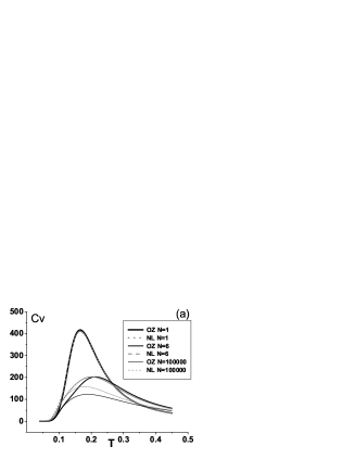
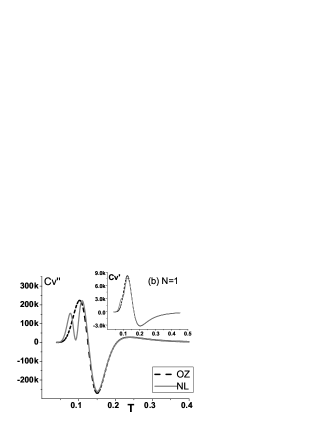
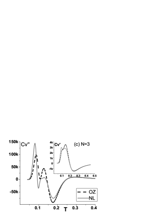
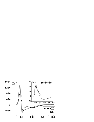
Figure 2: The figure shows specific heat $C_{v}$, $C^{\prime}_{v}$ (inset) and $C^{\prime\prime}_{v}$ as a function of $T$ for the logarithmic interaction (solid line) and $oz$ models (dashed line) for different values of $N$.

III Tapping

In tapping, the matrix is coupled to an external source, which is then removed and the number of different configurations (multiple solutions) are counted (Deo 9 ). The limit of external source $\rightarrow 0$ gives different moments which may result in different partition functions and hence free energies (considering different tappings explores entire space of the configurations). For the log model, the form of potential is $V(\sigma)=[\frac{\mu}{2}\sigma^{2}-\frac{t^{\prime\prime}}{2}(\log\sigma^{2})]$ with $\lambda_{i}$ as the eigenvalues of $\sigma$. Introducing a linear matrix source $\sigma/y$ in the action of Eq. (1) (after solving), the saddle points are found from the equation $\frac{\partial[V(\lambda_{i})-\frac{1}{y}\lambda_{i}]}{\partial\lambda_{i}}=0$ to be

$$\sigma_{c}=\frac{\frac{1}{\mu y}\pm\sqrt{\frac{1}{\mu^{2}y^{2}}+\frac{4t^{\prime\prime}}{\mu}}}{2}$$ (15)

where $\mu=1/v$ and $t^{\prime\prime}=1/w$. Depending upon small or large $1/y$, the saddle points are

$$\sigma = +\sqrt{\frac{t^{\prime\prime}}{\mu}}+\frac{1}{2}(\frac{1}{\mu w})\;;\;\frac{1}{y}>0.$$ (16)

$$\sigma = -\sqrt{\frac{t^{\prime\prime}}{\mu}}+\frac{1}{2}(\frac{1}{\mu w})\;;\;\frac{1}{y}<0.$$ (17)

The action $S(\sigma)=\frac{\mu}{2}\sigma^{2}-\frac{t^{\prime\prime}}{2}log(\sigma^{2})-\frac{1}{y}\sigma$ therefore becomes

$$S(\sigma^{\pm}_{c})=\frac{t^{\prime\prime}}{2}[1-log(\frac{t^{\prime\prime}}{\mu})]\mp\sqrt{\frac{t^{\prime\prime}}{\mu}}\frac{1}{y}.$$ (18)

Thus the set of moments grows exponentially as $2^{N/2}$. This suggests the intriguing possibility that log interaction matrix model (and also $oz$) represent a class of ‘glassy’ matrix models.

IV Conclusions

The Letter studies a Penner type logarithmic interaction in the framework of a random matrix model of RNA folding and its structure combinatorics. This is the first instance where Penner matrix models have been applied to the study of RNAs. The asymptotic analysis suggests: (i) There exists different regions of $N$ in which the structural properties of the log interaction model (and also the $oz$) are different. (ii) A dependence of the combinatoric factor on the matrix size $N$ is found for the matrix models of RNA with and without interactions which has not been found before. (iii) The effect of interaction is visible in $v$ and $N$ which is given by the re-scaling of $v$ to twice that in the $oz$ (for large $N$ region) and dominated by $N$ (in the small $N$ region). The substitution $v/2$ in the log partition function at large $N$, reduces the structures to that found for the $oz$ model. (iv) The $L^{3g-3/2}$ behavior for large $N$ in the log interaction model is in good agreement with the $oz$ model. For small $N$, these exponents change as the secondary region is stretched longer while the tertiary region gets shortened. The effect of interaction is thus visible in the way the structures are distributed for a given length which may represent a new universality class, Fig. 1(b) 8 . The specific heat clearly highlights the different structural behavior in the two regions of $N$ with an unusual double peak for $N=1$ and a kink for large $N$. The tapping explicitly shows the presence of multiple solutions in these matrix models. An important necessary direction in these models is the derivation of the generating function with any $N^{\prime}t^{\prime}$. This will help clarify some unresolved issues such as the genus characterization (which at the moment is indistinguishable from effect of interaction both of which are contained in $N$). The matrix model of RNA with logarithmic interaction provides a larger class of interacting RNA structures than the matrix model of 3 ; 4 ; 5 ; 6 . This is because an additional (and therefore complete) dependence of the structures on $n$ (other than vertices and edges) in the model will be possible in terms of all the $n$ punctures of the Riemann surfaces.

We thank Professor Henri Orland. We thank CSIR and UGC for senior and junior research fellowships and the University faculty R&D research program for financial support.

References

- (1) M. S. Waterman, Stud. Appl. Math. 60, 91 (1979); C. Haslinger and P. F. Stadler, Bull. Math. Biol. 61, 437 (1999); T. Akutsu, Discret. Appl. Math. 104, 45 (2000); E. Y. Jin and C. M. Reidys, Bull. Math. Biol. 70, 45 (2008); T. J. X. Li and C. M. Reidys, Preprint arXiv:1006.2924; references therein.
- (2) Henri Orland and A. Zee, Nucl. Phys. B 620, 456 (2002).
- (3) G. Vernizzi, H. Orland, and A. Zee, Phys. Rev. Lett. 94, 168103 (2005).
- (4) I. Garg and N. Deo, Pramana J. Phys. 73, 533 (2009).
- (5) I. Garg and N. Deo, Phys. Rev. E 79, 061903 (2009).
- (6) I. Garg and N. Deo, Eur. Phys. J E 33, 359 (2010).
- (7) A. Pagnani, G. Parisi, and F. Ricci-Tersenghi, Phys. Rev. Lett. 84, 2026 (2000); R. Bundschuh and T. Hwa, Phys. Rev. E 65, 031903 (2002); references therein.
- (8) K. Efetov, Supersymmetry in Disorder and Chaos, (Cambridge University Press, Cambridge, 1997); T. Guhr, A. Muller, and H. A. Weidenmuller, Phys. Rep. 299, 189 (1998); P. J. Forrester, N. C. Snaith, and J. J. M. Verbaarschot, J. Phys. A: Math. Gen. 36, R1 (2003); F. Colomo and A. G. Pronko, J. Stat. Phys. 138, 662 (2010); J. Choi and K. A. Muttalib, Phys. Rev. B 82, 104202 (2010); V. E. Kravtsov, in Handbook on Random Matrix Theory, (Oxford University Press, New York, 2010); Preprint arXiv:0911.0615; E. Bogomolny and O. Giraud, Phys. Rev. Lett. 106, 044101 (2011); references therein.
- (9) R. C. Penner, Bull. Am. Math. Soc. 15, 73 (1986); J. Diff. Geom. 27, 35 (1988); V. A. Kazakov, Mod. Phys. Lett. A 4, 2125 (1989): C. I. Tan, BROWN-HET-810 (1991); J. Distler and C. Vafa, Mod. Phys. Lett. A 6, 259 (1991); Chung-I Tan, Phys. Rev. D 45, 2862 (1992); L. Chekhov and Yu. Makeenko, Mod. Phys. Lett. A 14, 1223 (1992); N. Deo, J. Phys. A: Math. Gen. 36, 3617 (2003); N. Deo, Phys. Rev. E 68, 026130 (2003); S. Mukhi, Preprint hep-th/0310287; T. Eguchi and K. Maruyoshi, Preprint arXiv:0911.4797; R. J. Szabo and M. Tierz, J. Phys. A: Math. Theor. 43, 265401 (2010); references therein.
- (10) L. F. Cugliandolo, J. Kurchan, G. Parisi, and F. Ritort, Phys. Rev. Lett. 74, 1012 (1995); G. Parisi, Preprint arXiv: 9701032; L. F. Cugliandolo, J. Kurchan, and G. Parisi, ROM2F/94/27; references therein.