Multi-Time Multi-Scale Correlation Functions in Hydrodynamic Turbulence

Abstract

High Reynolds numbers Navier-Stokes equations are believed to break self-similarity concerning both spatial and temporal properties: correlation functions of different orders exhibit distinct decorrelation times and anomalous spatial scaling properties. Here, we present a systematic attempt to measure multi-time and multi-scale correlations functions, by using high Reynolds numbers numerical simulations of fully homogeneous and isotropic turbulent flow. The main idea is to set-up an ensemble of probing stations riding the flow, i.e. measuring correlations in a reference frame centered on the trajectory of distinct fluid particles (the quasi-Lagrangian reference frame introduced by Belinicher & L’vov, Sov. Phys. JETP 66, 303 (1987)). In this way we reduce the large-scale sweeping and measure the non-trivial temporal dynamics governing the turbulent energy transfer from large to small scales. We present evidences of the existence of dynamic multiscaling : multi-time correlation functions are characterized by an infinite set of characteristic times.

I Introduction

A comprehensive theory of the Eulerian and Lagrangian statistical properties of turbulence is one of the outstanding open problems in classical physics frisch:1995 . Most studied quantities concerns either measurements performed at the same time in multiple positions (Eulerian measurements) sreenivasan:1997 ; gotoh:2009 , or along one or several particles moving with the flow (Lagrangian measurements) yeung:2002 ; toschi:2009 ; benzi:jfm:2010 . The latter are optimal to study temporal properties of the underlying turbulent flows mordant:2001 ; arneodo:2008 but cannot simultaneously disentangle also spatial fluctuations, being based on single point, as for the case of acceleration laporta:2001 ; sawford:2003 ; biferale:2005a ; berg:2006a , or on a evolving set of scales as for two-particles sawford:2001 ; biferale:2005b ; bourgoin:2006 ; berg:2006b ; salazar:2009 and multi-particle dispersions biferale:2005c ; xu:2008 . On the other hand, neither analytical control nor a firm phenomenological description of fully developed turbulence can be obtained without a solid understanding of the relation between spatio and temporal fluctuations borgas:1993 ; lvov:1997 ; biferale:2004 ; chevillard:2006a ; zybin:2008 ; zybin:2010 ; benzi:pre:2009 ; yu:2009 ; kleimann:2009 ; stresing:2010 . In order to access unambiguously spatial and temporal fluctuations one needs to set the reference scale and to get rid of the large-scale sweeping in the same experimental –or numerical– set-up belinicher:1987 ; biferale:1999 ; mitra:2004 ; pandit:2008 . The idea here is to exploit numerical simulations to define a set of probes flowing with the wind, moving on a reference frame sticked with a representative fluid particle. In such a reference frame, we can access velocity fluctuations over different spatial resolution, together with their temporal evolution, without being affected by the large-scale sweeping wan:2010 . The interest of these measurements is twofold. First, all attempts to break the theoretical deadlock in turbulence have been hindered by the difficulties in closing both spatial and temporal fluctuations kraichnan:1974 ; lvov:1997 ; zybin:2010 (notice that the main theoretical breakthrough in turbulent systems have been obtained where temporal fluctuations are uncorrelated falkovich:2001 ). Second, small-scale parametrizations used for sub-grid turbulent closure call for more and more refined phenomenological understanding of spatial and temporal fluctuations meneveau:2000 .
In this article, we show that quasi-Lagrangian measurement are able to remove the sweeping effect, revealing that correlation times in the Eulerian and Lagrangian frame scale differently. Moreover, Lagrangian properties posses a dynamical multi-scaling, i.e. different correlation functions decorrelated with different characteristic time scales. The locality in space and time of the energy cascade is supported by studying the delayed peak in multi-time and multi-scale correlations. The main result we present is the confirmation of a theory lvov:1997 where a bridge between spatial and temporal intermittency was made by means of a refinement of the multifractal phenomenology (originally proposed for the spatial statistics of Eulerian velocity in parisifrisch:1985 ). Energy is transferred downscale with intermittent temporal fluctuations, and an associated infinite hierarchy of decorrelation times. Temporal fluctuations become wilder and wilder by decreasing the scale.

The article is organized as follows. In sec. II we present the numerical methods. In sec. III we show the result for single-scale multi-time correlation functions, for the bridge relation between temporal and spatial scaling exponents and for multi-time and multi-scale correlation functions.

$N^{3}$	$\delta x$	$\delta t$	$\nu$	$\overline{\varepsilon}$	$t_{tot}$	$N_{p}$	$M$	$\eta$	$\tau_{\eta}$	$u_{rms}$	$\lambda$	$L$	$T$	$Re_{\lambda}$
$256^{3}$	$2.4\!\cdot\!10^{-2}$	$5\!\cdot\!10^{-4}$	$3\!\cdot\!10^{-3}$	$1.0$	110	$3.2\!\cdot\!10^{4}$	$20$	$1.28\!\cdot\!10^{-2}$	$5.48\!\cdot\!10^{-2}$	$1.41$	$3.00\!\cdot\!10^{-1}$	$4.24$	$3.00$	$141$
$512^{3}$	$1.2\!\cdot\!10^{-2}$	$4\!\cdot\!10^{-4}$	$2.05\!\cdot\!10^{-3}$	$0.9$	12	$1.024\!\cdot\!10^{5}$	$20$	$9.89\!\cdot\!10^{-3}$	$4.77\!\cdot\!10^{-2}$	$1.40$	$2.58\!\cdot\!10^{-1}$	$4.56$	$3.26$	$176$

Table 1: DNS parameters: $N$ is the number of grid points per spatial direction; $\delta x=2\pi/N$ and $\delta t$ are the spatial and temporal discretization; $\nu$ is the value of kinematic viscosity; $\overline{\varepsilon}$ the mean value of the energy dissipation rate. $t_{tot}$ is the total simulation time; $N_{p}$ total number of fluid tracers; $M$ number of probes at fixed distances from tracer particle; $\eta=(\nu^{3}/\overline{\varepsilon})^{1/4}$ and $\tau_{\eta}=(\nu/\overline{\varepsilon})^{1/2}$ the Kolmogorov dissipative spatial and temporal scales, $u_{rms}=\left(\overline{\langle u_{i}u_{i}\rangle}_{V}/3\right)^{1/2}$ the single-component root-mean-square velocity, $\lambda=(15\ \nu\ u_{rms}^{2}/\varepsilon)^{1/2}$ the Taylor micro-scale, $T=(3/2)u_{rms}^{2}/\overline{\varepsilon}$ and $L=u_{rms}\,T$ large-eddy-turnover temporal and spatial scales; $Re_{\lambda}=u_{rms}\ \lambda/\ \nu$ the Taylor scale based Reynolds number.

II Methods

II.1 Sweeping and quasi-Lagrangian reference

The difficulty in studying the temporal correlations in turbulence is associated with the sweeping of small scales by means of larger ones. In the case of a flow with a “large” mean velocity ${\bf U}$, fluctuations ${\bf u}^{\prime}\equiv{\bf u}-{\bf U}$ are almost passively transported in space via the Galilean transformation ${\bf x}^{\prime}(t)={\bf x}+{\bf U}t$. This property, dubbed Taylor frozen flow hypothesis, is commonly used in experiments to remap the hot-wire probe readings (which are done in time) to measurements in space and is supposed to be valid as long as turbulence levels are small ($|{\bf u}^{\prime}|/|{\bf U}|\ll 1$). In order to study the temporal evolution of velocity differences at a given scale $r$ it is hence necessary to get rid of large-scale (infra-red) effects. This can be done by “riding the flow”, i.e. by sticking the origin of the reference frame on the position of a fluid parcel moving in the flow (see sketch in fig. 1). Such reference frame, introduced by Belinicher and L’vov belinicher:1987 , is called quasi-Lagrangian. Because of this difficulty, measures of the quasi-Lagrangian type have been performed only numerically at moderate Reynolds and for small-scale quantities schumacher:2010 or at high Reynolds in turbulence models, such as shell models (where sweeping is absent biferale:1999 ; lohse:2000 ; mitra:2004 ; pandit:2008 ).

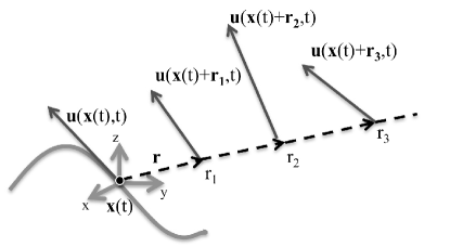
Figure 1: Sketch of the ${\bm{r}}_{i}$ probes “riding the flow”, i.e., at fixed positions in a reference frame moving sticked with a representative fluid particle ${\bf x}(t)$.

II.2 Numerical methods

In the present study we measure multi-scale and multi-time correlations in a quasi-Lagrangian reference frame from fully resolved high-statistics three-dimensional Direct Numerical Simulations (DNS) of homogeneous and isotropic turbulence. We evolve the incompressible Navier-Stokes (NS) equations:

$$\partial_{t}{\bf u}+({\bf u}\cdot\nabla){\bf u}=-\nabla p+\nu\Delta{\bf u}+{\bf f}\,,\quad\nabla\cdot{\bf u}=0\,,\,$$ (1)

in a cubic three-periodic domain via a pseudo-spectral algorithm and $2^{nd}$ order Adams-Bashforth time marching. The forcing ${\bf f}$, defined as in lamorgese:2004 , acts only on the first two shells in Fourier space ($|{\bf k}|\leq 2$) and keeps constant in time the total (volume averaged) injected power, $\langle{\bf f}\cdot{\bf u}\rangle_{V}=\textrm{const.}$ We report data coming from a set of simulations with $N^{3}=256^{3}$ and $512^{3}$, corresponding to $\mathrm{Re}_{\lambda}\,\simeq\,140$ and $180$ respectively (see Table 1 for relevant parameters characterizing the flows). The simulation e.g. at $\mathrm{Re}_{\lambda}\,\simeq\,140$ has been carried on for $40$ Eulerian turnover times, $T=(3/2)u_{rms}^{2}/\overline{\varepsilon}$. We also integrated numerically $N_{p}=3.2\cdot 10^{4}$ tracers evolving with the local Eulerian velocity field $\dot{{\bf x}}(t)={{\bf u}({\bf x}(t),t)}$. At fixed temporal intervals we evaluate the fluid velocity also at ${\bm{x}}(t)+{\bm{r}}_{i}$, with $i=0,\ldots,M$ (spatial distances from each tracer). The vectors are chosen to be always along one fixed direction, $\hat{{\bf r}}$, and are logarithmically spaced in the range between zero and half of the box-size (we use $M=20$), see figure 1. Similar measurements are done also at fixed positions uniformly spaced in the fluid domain. These two set of data are denoted respectively as quasi-Lagrangian (${L}$) and Eulerian (${E}$).

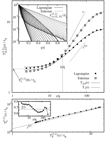
Figure 2: Top-inset: Correlation functions of single-scale velocity differences $C_{r,r[{L},{E}]}^{(1,1)}(\tau)$ as a function of the time delay $\tau$, in the (quasi-)Lagrangian (solid line) and Eulerian (dashed line) frame of reference. Top-main panel: Single-scale integral correlation time $T^{(1,1)}_{{L}}(r)$ ($\bullet$) and $T^{(1,1)}_{{E}}(r)$ ($\Box$) estimated from Lagrangian and Eulerian $C_{r,r}^{(1,1)}(\tau)$ correlations. The straight lines indicate slopes $2/3$ and $1$. The fit using the function $T_{n}(r)$ discussed in the text with $n=2/3$ (solid) and $n=1$ (dashed line) are also shown. Vertical dotted line reports the value $\lambda\simeq 20\eta$ for which both correlation times are $\sim\tau_{\eta}$. The horizontal line show the integral correlation time of longitudinal velocity gradients $T^{(1,1)}_{{L}}(\nabla_{||}{\bf u})=2.15\ \tau_{\eta}$ along Lagrangian trajectories, which corresponds to the small-scale(ultra-violet) limit, $\lim_{r\to 0}T^{(1,1)}_{{L}}(r)$. Bottom main panel: Extended Self Similarity plot: $T^{(1,1)}_{{L}}(r)\ vs.\ T^{(1,1)}_{{E}}(r)$ and its local slope: $d\log{T_{{L}}^{(1,1)}(r)}/d\log{T_{{E}}^{(1,1)}(r)}$ (Bottom inset). The inertial range behavior $\sim r^{2/3}$ is reported in both panels.

II.3 Notations and Measurements

We focus our attention on the longitudinal increments of velocity differences across a displacement ${\bf r}$:

$$\delta u_{{\bf r}}(\tilde{{\bf x}},t)=\left({\bf u}(\tilde{{\bf x}}+{\bf r},t)-{\bf u}(\tilde{{\bf x}},t)\right)\cdot\hat{{\bf r}}.$$ (2)

Notice that we have adopted a unifying notation, for us $\tilde{{\bf x}}$ can represent either a fixed point in space $\tilde{{\bf x}}={\bf x}_{0}$ or a point following a fluid particle: $\tilde{{\bf x}}={\bf x}(t)=\int_{t_{0}}^{t}{\bf u}({\bf x}(t|{{\bf x}}_{0},t_{0}),t)\,dt+{\bf x}_{0}$ (a trajectory passing from ${\bf x}_{0}$ at time $t_{0}$). We distinguish between the two cases by the superscript labels: $\delta u_{{\bf r}}^{{E}}(\tilde{{\bf x}},t)$ or $\delta u_{{\bf r}}^{{L}}(\tilde{{\bf x}},t)$. Note that $\overline{\left(\delta u_{{\bf r}}^{{E}}\right)^{p}}$, with overbar denoting time average, is the usual Eulerian structure function of order $p$, furthermore by means of ergodicity it can be proved that $\overline{\left(\delta u_{{\bf r}}^{{E}}\right)^{p}}=\overline{\left(\delta u_{{\bf r}}^{{L}}\right)^{p}}$ (therefore for such a quantity ${E}$, ${L}$ labels will be dropped). We define the generic multi-scale, multi-time correlation functions lvov:1997 :

$$C_{R,r\,[{L},{E}]}^{(q,p-q)}(\tau)=\frac{\overline{\left(\delta u_{{\bf R}}^{[{L},{E}]}(t)\right)^{q}\cdot\left(\delta u_{{\bf r}}^{[{L},{E}]}(t+\tau)\right)^{p-q}}}{\overline{(\delta u_{{\bf R}}(t))^{q}\cdot(\delta u_{{\bf r}}(t))^{p-q}}},$$ (3)

where ${\bf R}$ and ${\bf r}$ denote separation vector fixed in space and with different magnitude. Note that the ${L},{E}$ distinction must be kept for the average of the multi-time product in the numerator. Given the correlation functions we can define an Eulerian and Lagrangian (integral) correlation time as follows lvov:1997 :

$$T^{(q,p-q)}_{[{L},{E}]}(R,r)=\int_{0}^{+\infty}C_{R,r\,[{L},{E}]}^{(q,p-q)}(\tau)\ d\tau.$$ (4)

III Results

III.1 Single-scale multi-time correlation

We begin discussing the special case of a single-scale, multi-time correlation, i.e. $R=r$. Dimensional inertial-range scaling, $\overline{\left(\delta u_{{\bf r}}\right)^{p}}\sim(\varepsilon\,r)^{p/3}$, provides the following estimate for the turnover time of inertial eddies of size $r$, $T^{(q,p-q)}_{{L}}(r)\sim r/\left(\overline{\left(\delta u_{{\bf r}}\right)^{p}}\right)^{1/p}\sim r^{2/3}$. On the contrary the Eulerian correlation time -due to sweeping effect- can be estimated by means of the typical velocity difference of the largest eddy, which is proportional to the mean square root velocity, $\delta u_{{\bf L}}\sim u_{rms}$. One has $T^{(q,p-q)}_{{E}}(r)\sim r/\left(\overline{\left(\delta u_{{\bf L}}\right)^{p}}\right)^{1/p}\sim r/u_{rms}\sim r$. In the $r\to\eta$ limit both correlation times tend to the dissipative scale $\tau_{\eta}$. In Figure 2 (inset) we show the behavior of $C_{r,r}^{(1,1)}(\tau)$ for both Eulerian and quasi-Lagrangian velocity differences and for separation scales $r\in[2.4,245]\eta$. On the abscissa the time increment $\tau$ is made dimensionless through the Eulerian large eddy turnover time $T$ (see Tab.1). We clearly see that after a time $\sim T$ all the correlations have decreased at least of a factor 50, supporting the quality and convergence of our measurements. The main panel of Figure 2 shows the integral correlation times both for the Eulerian and quasi-Lagrangian case as computed from (4), in a time integration window $[0,T]$. The behavior is in qualitative agreement with the expected scaling, the Lagrangian case being less steep than the Eulerian one, however pure power-law scaling seems to be hindered by finite Reynolds number and system finite-size effects. To demonstrate this, we introduce a parametrization for the second order spatial velocity structure functions, with dissipative and large-scale cut-off (see also lohse:2000 ): $T_{n}(r)=c_{1}(1+(r/c_{2})^{2})^{n/2}(1+(r/c_{3})^{2})^{-n/2}$ with $n=2/3$ and $n=1$ respectively for the Lagrangian and Eulerian case. The parameters $c_{1},c_{2},c_{3}$ represent the dissipative correlation time scale, the dissipative and large cut-off scales, respectively. The good quality of the fit, shown in Fig. 2, supports our hypothesis. Plotting the Lagrangian correlation time as a function of the Eulerian one, a procedure similar to the Extended Self Similarity (ESS) benzi:1996 , does show a good scaling with slope $0.64\pm 0.02$ in the range $[20,200]\eta$, consistent with $2/3$ (Fig. 2). This finding again supports the idea that the limited scaling in Figure 2 is due to finite Reynolds effects.

III.2 Intermittency and test of the bridge relations

It is well known that Eulerian statistics shows intermittent corrections to dimensional scaling. For example, for structure function we have $\overline{\left(\delta u_{{\bf r}}\right)^{p}}\sim r^{\zeta(p)}$ where $\zeta(p)$ is a nonlinear convex function of $p$ frisch:1995 . In 1997, L’vov, Podivilov & Procaccia lvov:1997 provided a possible framework to encompass the phenomenology associated to intermittency also to temporal fluctuations. The idea consists in noticing that for time correlations the structure of the advection term of the Navier-Stokes equations suggests the relation: $T^{(q,p-q)}_{{L}}(r)\sim r/\left(\overline{\left(\delta u_{{\bf r}}\right)^{p}}\,/\,\overline{\left(\delta u_{{\bf r}}\right)^{p-1}}\right)\sim r^{z(p)}$ lvov:1997 . Using the scaling for the Eulerian quantities, $\overline{\left(\delta u_{{\bf r}}\right)^{p}}\sim r^{\zeta(p)}$ one gets to the so-called bridge relations (BR) connecting spatial and temporal properties:

$$z(p)=1-\zeta(p)+\zeta(p-1).$$

Similar idea have also been successfully applied to connect the statistics of acceleration and velocity gradients biferale:2004 . Plugging the empirical values gotoh:2009 ; benzi:jfm:2010 for the Eulerian exponents in the previous expression, one predicts $z(p)=0.67,0.74,0.78,0.80(\pm 0.01)$ for the orders $p=2,4,6,8$ respectively. In Figure 3 (main top panel) the different moments of the Lagrangian integral times, i.e. $T_{{L}}^{(q,p-q)}(r)$ (with $p-q=1$), are shown versus the scale $r$. A steepening of the scaling properties with increasing $p$ can be noticed.

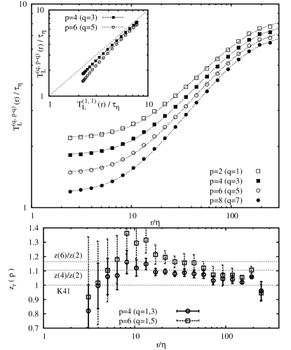
Figure 3: Test of dynamic multiscaling. Top panel: $T^{(q,p-q)}_{{L}}(r)$ $vs.$ $r/\eta$, with $p=2,4,6,8$ and $q=p-1$. Inset top panel: ESS-like plot of $T^{(q,p-q)}_{{L}}(r)\,vs.\,T^{(1,1)}_{{L}}(r)$ for $p=4,6$, $q=p-1$. Bottom panel: local scaling exponents, $z_{r}(p)$, for $p=4,6$ and $q=p-1,1$. Central values are computed as the mean between $q=p-1$ or $q=1$ for each $p$ value. Error bars gives the dispersion between the two choices. Horizontal lines represents from bottom to top respectively the dimensional prediction $z(p)/z(2)=1$, $\forall p$ denoted as $K41$, and the BR values $z(4)/z(2)=0.74/0.67$ and $z(6)/z(2)=0.78/0.67$.

In order to enhance the quality of the measurements we resort to ESS procedure by plotting a generic $T_{{L}}^{(q,p-q)}(r)$ versus $T_{{L}}^{(1,1)}(r)$ (see inset of Figure 3) in log-scale. It is now possible to define local scaling exponents as:

$$z_{r}(p)=d\log{T_{{L}}^{(q,p-q)}(r)}/d\log{T_{{L}}^{(1,1)}(r)},$$

which according to the BR should scale as $z(p)/z(2)$ for $r$ in the inertial range. The result of this local scaling exponent analysis is shown in Figure 3 (bottom panel) for the orders $p=4,6$. Notice that the BR predicts the same scaling properties independently of $q$. In our numerics we find slightly different results for $q=1$ or $q=p-1$. The error bars in bottom panel of fig. (3) gives a quantitative estimate of the spread between the two results. In the inertial range $\sim[10,100]\eta$ we find some deviation from the K41 values $z(p)/z(2)=1$, consistent with the BR predictions for $p=4,6$. We notice that the predicted intermittent corrections are very small and error bars large. Higher statistics and/or higher Reynolds number may help in giving stronger confirmation to these evidences.

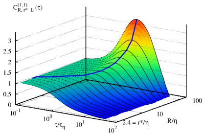
Figure 4: Top panel: $C_{R,r^{*}\,L}^{(1,1)}(\tau)$ for fixed $r^{*}=2.4\eta$ at changing $R\in[r^{*}:120\eta]$. The solid line is a guide to the eyes connecting the peak for each given $R$. Inset bottom panel: Cut of $C_{R,r^{*}\,L}^{(1,1)}(\tau)$ at increasing $R$ (from bottom to top) as a function of $\tau$. Symbol ($\bullet$) marks the position of the maximal correlation value (denoted as $T^{(1,1)}_{peak}(R)$) which increases for increasing values of $R$. Bottom panel: Comparison between $T^{(1,1)}_{peak}(R)$ and $T^{(1,1)}_{{L}}(R)-T^{(1,1)}_{{L}}(r^{*})$. The inertial scaling $R^{2/3}$ is also drawn for comparison.

III.3 Multi-scale multi-time correlation

We now focus on the most general case of multi-scale and multi-time correlation functions in the Lagrangian frame. In particular, in the correlation function (3) we vary the large scale $R$ while the small scale $r$ is kept fixed $r\simeq\eta$. Note that the velocity difference $\delta u_{{\bf R}}$ precedes in time the difference $\delta u_{{\bf r}\simeq\eta}$. We are therefore interested in the time it takes for a velocity fluctuation to cascade down from a large eddy (of size $R$) to the smallest one (of size $\sim\eta$). In Figure 4 (top panel) we show the correlations $C_{R,r^{*}\,{L}}^{(1,1)}(\tau)$ with $r^{*}=2.4\,\eta$ as defined from Eqn. (3) (except for the fact that to enhance the contrast instead of $\delta u_{{\bf r}}$ we used $|\delta u_{{\bf r}}|$ ). The presence of a peak in $C_{R,r^{*}\,{L}}^{(1,1)}(\tau)$ for each given $R$, defines a time, $T^{(1,1)}_{peak}(R)$, which increases for increasing values of $R$. The presence of the peak can be directly associated with the time lapse it takes the energy to go down through scales from $R$ to $r^{*}$, i.e. a direct evidence of temporal properties of the Richardson turbulent cascade frisch:1995 . In the inset of the bottom panel we show the curves corresponding to $C_{R,r^{*}\,{L}}^{(1,1)}(\tau)$, for each different $R$ at varying $\tau$.
The scaling behavior of the peak time $T^{(1,1)}_{peak}(R)\sim R^{2/3}$, shown in Fig. 4 (bottom panel), is in agreement with what has been measured for Fourier-space based quantities by Wan et al. in wan:2010 .
Also in figure 4 (bottom panel) a comparison of $T^{(1,1)}_{peak}(R)$ with $T^{(1,1)}_{{L}}(R)-T^{(1,1)}_{{L}}(r^{*})$ (as computed for Fig. 2) is shown. It is remarkable to note that the amplitude and scaling of $T^{(1,1)}_{peak}(R)$ -coming from the multi-scale correlation function- is close and compatible with $T^{(1,1)}_{{L}}(R)-T^{(1,1)}_{{L}}(r^{*})$ -coming from the single-scale correlation functions. This finding provides a clean confirmation that energy is transferred down-scale in the quasi-Lagrangian reference frame.

IV Conclusions

We presented an investigation of multi-scale and multi-time velocity correlations in hydrodynamic turbulence in Eulerian and quasi-Lagrangian reference frame. Our main results are the following: i) We have demonstrated that quasi-Lagrangian measurement are able to remove the sweeping effect. The integral correlation times in the Eulerian and Lagrangian frame are shown to scale differently. ii) Lagrangian properties posses a dynamical multi-scaling, i.e. different correlation functions decorrelated with different characteristic time scales. iii) Bridge relations connecting single-time multi-scale exponents with multi-time single-scale exponents are valid, within numerical accuracy. iv) The locality in space and time of the energy cascade is supported by studying the delayed peak in multi-time and multi-scale correlations. Temporal fluctuations becomes larger and larger by going to smaller and smaller scales, a phenomenon that may even affect numerical stability criteria for time marching, similarly to an effect concerning spatial resolution induced by spatial intermittency schumacher:2007 . Some issues similar to the ones here discussed have also been addressed in a recent numerical study wan:2010 where evidences of the Lagrangian nature of the turbulent energy cascade have been demonstrated by studying the correlation between energy dissipation and local energy fluxes in the quasi-Lagrangian frame. While the method followed in wan:2010 requires a knowledge of the three-dimensional velocity field, the approach proposed in the present manuscript needs only the knowledge of the velocity at just a few points along a Lagrangian trajectory: a measurements which may be already accessible in current particle tracking experimental set-ups.

Acknowledgments The authors acknowledge useful discussions with R. Pandit and P. Perlekar. E.C. wish to thank J.-F. Pinton for discussions and support to the initial stages of this work. E.C. has been supported also by the HPC-EUROPA2 project (project number: 228398) with the support of the European Commission - Capacities Area - Research Infrastructures. We acknowledge COST Action MP0806 and computational support from SARA (Amsterdam, The Netherlands), CINECA (Bologna, Italy) and CASPUR (Rome, Italy).

References

- (1) U. Frisch, Turbulence: The Legacy of A. N. Kolmogorov (Cambridge University Press, Cambridge, 1995).
- (2) K. R. Sreenivasan and R. A. Antonia, The phenomenology of small-scale turbulence, Ann. Rev. Fluid Mech. 29, 435 (1997).
- (3) T. Ishihara, T. Gotoh, and Y. Kaneda, Study of High-Reynolds Number Isotropic Turbulence by Direct Numerical Simulation, Ann. Rev .Fluid Mech. 41, 165 (2009).
- (4) P. K. Yeung, Lagrangian investigations of turbulence, Ann. Rev. Fluid Mech. 34, 115 (2002).
- (5) F. Toschi and E. Bodenschatz, Lagrangian properties of particles in Turbulence, Ann. Rev. Fluid Mech. 41, 375 (2009).
- (6) R. Benzi, L. Biferale, R. Fisher, D. Q. Lamb, and F. Toschi, Inertial range Eulerian and Lagrangian statistics from numerical simulations of isotropic turbulence, J. Fluid Mech. 653, 221 (2010).
- (7) N. Mordant, P. Metz, O. Michel, and J. F. Pinton, Measurement of Lagrangian Velocity in Fully Developed Turbulence, Phys. Rev. Lett. 87, 214501 (2001).
- (8) A. Arneodo, R. Benzi, J. Berg, L. Biferale, E. Bodenschatz, and et al., Universal Intermittent Properties of Particle Trajectories in Highly Turbulent Flows, Phys. Rev. Lett. 100, 254504 (2008).
- (9) A. L. Porta, G. A. Voth, A. M. Crawford, J. Alexander, and E. Bodenschatz, Fluid particle accelerations in fully developed turbulence, Nature 409, 1017 (2001).
- (10) B. L. Sawford, P. K. Yeung, M. S. Borgas, P. Vedula, A. L. Porta, A. M. Crawford, and E. Bodenschatz, Conditional and unconditional acceleration statistics in turbulence, Phys. Fluids 15, 3478 (2003).
- (11) L. Biferale, G. Boffetta, A. Celani, A. Lanotte, and F. Toschi, Particle trapping in three-dimensional fully developed turbulence, Phys. Fluids 17, 021701 (2005).
- (12) J. Berg, Lagrangian one-particle velocity statistics in a turbulent flow, Phys. Rev. E 74, 016304 (2006).
- (13) B. Sawford, Turbulent relative dispersion, Ann. Rev. Fluid Mech. 33, 289 (2001).
- (14) L. Biferale, G. Boffetta, A. Celani, B. J. Devenish, A. Lanotte, and F. Toschi, Lagrangian statistics of particle pairs in homogeneous isotropic turbulence, Phys. Fluids 17, 115101 (2005).
- (15) M. Bourgoin, N. T. Ouellette, H. Xu, J. Berg, and E. Bodenschatz, The Role of Pair Dispersion in Turbulent Flow, Science 311, 835 (2006).
- (16) J. Berg, B. Luthi, J. Mann, and S. Ott, Backwards and forwards relative dispersion in turbulent flow: an experimental investigation, Phys. Rev. E 74, 016304 (2006).
- (17) J. P. L. C. Salazar and L. R. Collins, Two-Particle Dispersion in Isotropic Turbulent Flows, Ann. Rev. Fluid Mech. 41, 405 (2009).
- (18) L. Biferale, G. Boffetta, A. Celani, B. J. Devenish, A. Lanotte, and F. Toschi, Multiparticle dispersion in fully developed turbulence, Phys. Fluids 17, 111701 (2005).
- (19) H. Xu, N. T. Ouellette, and E. Bodenschatz, Evolution of geometric structures in intense turbulence, New J. Phys. 10, 013012 (2008).
- (20) M. S. Borgas, The Multifractal Lagrangian Nature of Turbulence, Phil. Trans.: Physical Sciences and Engineering 342, 379 (1993).
- (21) V. L’vov, E. Podivilov, and I. Procaccia, Temporal multiscaling in hydrodynamic turbulence, Phys Rev E 55, 7030 (1997).
- (22) L. Biferale, G. Boffetta, A. Celani, B. J. Devenish, A. Lanotte, and F. Toschi, Multifractal statistics of Lagrangian velocity and acceleration in turbulence, Phys. Rev. Lett. 93, 064502 (2004).
- (23) L. Chevillard and C. Meneveau, Lagrangian Dynamics and Statistical Geometric Structure of Turbulence, Phys. Rev. Lett. 97, 174501 (2006).
- (24) K. Zybin, V. Sirota, A. Ilyin, and A. Gurevich, Lagrangian statistical theory of fully developed hydrodynamical turbulence, Phys. Rev. Lett. 100, 174504 (2008).
- (25) K. P. Zybin and V. A. Sirota, Lagrangian and Eulerian Velocity Structure Functions in Hydrodynamic Turbulence, Phys. Rev. Lett. 104, 154501 (2010).
- (26) R. Benzi, L. Biferale, E. Calzavarini, D. Lohse, and F. Toschi, Velocity gradients along particles trajectories in turbulent fows: the refined similarity hypothesis in the Lagrangian frame, Phys. Rev. E 80, 066318 (2009).
- (27) H. Yu and C. Meneveau, Lagrangian Refined Kolmogorov Similarity Hypothesis for Gradient Time-evolution in Turbulent Flows, Phys. Rev. Lett. 104, 084502 (2010).
- (28) J. Kleimann, A. Kopp, H. Fichtner, and R. Grauer, Statistics of a mixed Eulerian-Lagrangian velocity increment in fully developped turbulence, Physica Scripta 79, 055403 (2009).
- (29) R. Stresing and J. Peinke, Towards a stochastic multi-point description of turbulence, New Journal of Physics 12, 103046 (2010).
- (30) V. I. Belinicher and V. S. L’vov, A scale-invariant theory of developed hydrodynamic turbulence, Sov. Phys. JETP 66, 303 (1987).
- (31) L. Biferale, G. Boffetta, A. Celani, and F. Toschi, Multi-time, multi-scale correlation functions in turbulence and in turbulent models, Physica D 127, 187 (1999).
- (32) D. Mitra and R. Pandit, Varieties of dynamic multiscaling in fluid turbulence, Phys Rev Lett 93, 024501 (2004).
- (33) R. Pandit, S. S. Ray, and D. Mitra, Dynamic multiscaling in turbulence, Eur. Phys. J. B 64, 463 (2008).
- (34) M. Wan, Z. Xiao, C. Meneveau, G. L. Eyink, and S. Chen, Dissipation-energy flux correlations as evidence for the Lagrangian energy cascade in turbulence, Phys Fluids 22, 061702 (2010).
- (35) R. H. Kraichnan, On Kolmogorov’s inertial-range theories, J. Fluid Mech. 62, 305 (1974).
- (36) G. K. Falkovich G and V. M, Particles and fields in fluid turbulence, Rev. Mod. Phys. 73, 913 (2001).
- (37) C. Meneveau and J. Katz, Scale-invariance and turbulence models for large-eddy simulation, Ann. Rev. Fluid Mech. 32, 1 (2000).
- (38) G. Parisi and U. Frisch, On the singularity structure of fully developed turbulence, Turbulence and Predictability in Geophysical Fluid Dynamics, edited by M. Ghil, R. Benzi, and G. Parisi 84 (1985).
- (39) J. Schumacher, Sub-Kolmogorov-scale fluctuations in fluid turbulence, EuroPhys. Lett 80, 54001 (2007).
- (40) J. Schumacher, B. Eckhardt, and C. R. Doering, Extreme vorticity growth in Navier Stokes turbulence, Physics Letters A 374, 861 (2010).
- (41) S. Grossmann, D. Lohse, and A. Reeh, Multiscale correlations and conditional averages in numerical turbulence, Phys. Rev. E 61, 5195 (2000).
- (42) A. G. Lamorgese, D. A. Caughey, and S. B. Pope, Direct numerical simulation of homogeneous turbulence with hyperviscosity, Phys. Fluids 17, 015106 (2004).
- (43) R. Benzi, L. Biferale, S. Ciliberto, M. Struglia, and R. Tripiccione, Generalized scaling in fully developed turbulence, Physica D 96, 162 (1996).