FTUV-11-0324

IFUM-971-FT

KA-TP-08–2011

LPN11-14

SFB/CPP-11-14

$W^{\pm}\gamma\gamma$ production with leptonic decays at NLO QCD
G. Bozzi¹, F. Campanario², M. Rauch² and D. Zeppenfeld^{2 1} Dipartimento di Fisica, Università di Milano and INFN, Sezione di Milano
Via Celoria 16, I-20133 Milano, Italy
² Institut für Theoretische Physik, Universität Karlsruhe, KIT,
76128 Karlsruhe, Germany

The computation of the ${\cal O}(\alpha_{s})$ QCD corrections to the cross sections for $W^{\pm}\gamma\gamma$ production in hadronic collisions is presented. We consider the case of real photons in the final state, but include full leptonic decays of the $W$. Numerical results for the LHC and the Tevatron are obtained through a parton level Monte Carlo based on the structure of the VBFNLO program, allowing an easy implementation of general cuts and distributions. We show the dependence on scale variations of the integrated cross sections and provide evidence of the fact that NLO QCD corrections strongly modify the LO predictions for observables at the LHC both in magnitude and in shape.

— 22:05

1 Introduction

Precise and reliable predictions of cross sections at hadron colliders require the calculation of higher order QCD corrections. As part of such a program we have in the past determined next-to-leading-order (NLO) QCD corrections for the production cross sections of various combinations of three electroweak bosons, including $W^{+}W^{-}Z$ [1], $W^{\pm}W^{\mp}W^{\pm}$ and $W^{\pm}ZZ$ [2], $W^{+}W^{-}\gamma(ZZ\gamma)$ [3] and $W^{\pm}Z\gamma$ production [4]. In all cases, leptonic decays of the weak bosons were included in the calculations. For the production of three weak bosons, these results were verified against independent calculations [5, 6] which are available for on-shell weak bosons and neglecting Higgs boson exchange.

In the present paper, we present the ${\cal O}(\alpha_{s})$ QCD corrections for processes with two photons and one $W$ in the final state, namely the production of

$$"W^{+}\gamma\gamma"\qquad pp,\;p\bar{p}\to\nu_{l}l^{+}\gamma\gamma~{}+X$$

$$"W^{-}\gamma\gamma"\qquad pp,\;p\bar{p}\to l^{-}\bar{\nu}_{l}\gamma\gamma~{}+X\,.$$ (1.1)

A calculation of $W^{+}\gamma\gamma$ production at NLO QCD accuracy has been performed before [7], including the $q\to q\gamma$ fragmentation contributions. However, also Ref. [7] treats the $W$ as stable. By including off shell effects and, in particular, photon radiation from the final state charged lepton we aim at providing complementary information.

Processes involving two or three electroweak bosons in the final state are relevant for studying anomalous gauge interactions, as they give direct access to triple and quartic couplings [8]. $W^{\pm}\gamma\gamma$ production is sensitive to the $WW\gamma$ and $WW\gamma\gamma$ vertices. In addition, a final state with two photons and missing transverse energy is relevant in a variety of beyond the standard model scenarios [9]: in gauge-mediated supersymmetry breaking, for instance, the neutralino is often the next-to-lightest supersymmetric particle and decays into a photon plus a gravitino, giving a signal of two photons and missing $E_{T}$. In Ref. [10], a study of the background estimates for supersymmetry motivated di-photon production searches has been performed, pointing out the relevance of the $W^{\pm}\gamma\gamma$ production process as a standard model (SM) background in case of electron misidentification. Another possible application is an estimate of backgrounds when searching for $WH$ production, followed by Higgs decay to two photons.

The present work closely follows our previous calculations of NLO QCD corrections to triple electroweak boson production. In particular, photon isolation is implemented within the Frixione approach [11] and we, thus, avoid the need for the inclusion of $q\to q\gamma$ fragmentation contributions, which were discussed for $W^{+}\gamma\gamma$ production by Baur et al. [7]. Similar to previous work on triple weak boson production, we find that the QCD corrections are sizable and also modify the shape of the differential distributions for many observables: this proves that a simple rescaling of the LO results is not adequate and a full NLO Monte Carlo is needed for any quantitative determination of quartic couplings at the LHC. We have implemented our calculation within the VBFNLO framework [12], a parton level Monte Carlo program which allows the definition of general acceptance cuts and distributions.

The paper is organized as follows: in Section 2 we show the Feynman diagrams relevant for the calculation and provide an overview of the strategies used to compute the real and virtual corrections and the various checks performed to ensure the numerical accuracy of our code. In Section 3, we show numerical results, including the scale variations of the LO and NLO integrated cross sections and some selected differential distributions. Particular concern will be given to the consequences of approximate radiation zeroes which largely disappear when going from LO to NLO distributions, as was already emphasized in Ref. [7]. Conclusions are given in Section 4.

2 The calculation

Figure 1: Examples of the three topologies of Feynman diagrams contributing to the process $pp\to$$W^{\pm}\gamma\gamma$+ X   at tree-level.

For the calculation of virtual corrections, it is convenient to classify the contributing Feynman graphs according to the number of electroweak boson vertexes which are attached to the quark lines: graphs with three vertexes lead to pentagon loops, while boxes and triangles are the most complex structures for graphs with two or one electroweak vertex on the quark line. Examples for the three classes of diagrams contributing to $W^{\pm}\gamma\gamma$ production at Born level are shown in Fig. 1. Diagrams (a) and (b) exhibit the dependence on the quartic ($WW\gamma\gamma$) and triple ($WW\gamma$) gauge boson couplings.

As is customary in all VBFNLO calculations, we include the full spin correlations of the leptons coming from the $W$ decay and also the final state photon radiation off the charged leptons. As in all previous calculations, we have factorized the subgraphs involving boson splitting and decay into leptonic tensors [13], computed once per phase-space point in order to speed up the code, and we made use of the helicity technique introduced in Ref. [14] for the computation of matrix elements. The cancellation of infrared divergences coming from real and virtual corrections at NLO is achieved using the Catani-Seymour dipole subtraction method [15]. We note here that the strategy of separately computing the leptonic tensors proves particularly useful given the large number (372) of real emission diagrams at NLO.

For the real emission contributions, there is an additional issue to consider: the infrared singularity that may result from a photon emitted collinearly to a massless quark. The simple rejection of any event containing partons within a cone drawn around the photon direction would inevitably spoil the cancellation of infrared divergences for subprocesses with a gluon in the final state. As a solution, we use the photon isolation cut proposed by Frixione [11] which is described in more details in Section 3.

The NLO virtual corrections result from one-loop diagrams obtained by attaching a gluon line to the quark-antiquark line in diagrams like the ones depicted in Fig. 1. We combine the virtual corrections into three different groups, which include all loop diagrams derived from a given Born level configuration [13]. This leaves us with three universal building blocks, namely corrections to one, two or three vector bosons attached to the quark line. In all cases, the infrared divergent contributions factorize in terms of their corresponding Born amplitude and the full virtual term is given by

$$M_{V}=\widetilde{M}_{V}+\ \frac{\alpha_{S}}{4\pi}\ C_{F}\ \left(\frac{4\pi\mu^{2}}{Q^{2}}\right)^{\epsilon}\ \Gamma{(1+\epsilon)}\ \left[-\frac{2}{\epsilon^{2}}-\frac{3}{\epsilon}-8+\frac{4\ \pi^{2}}{3}\right]\ M_{B},$$ (2.1)

where $Q$ is the partonic center-of-mass energy, i.e. the invariant mass of the $W^{\pm}\gamma\gamma$ system, $M_{B}$ the total born contribution, and the term $\widetilde{M}_{V}$ includes the finite parts of the virtual corrections to 2 and 3 weak boson amplitudes which we call virtual-box and virtual-pentagons in the following, so named since boxes and pentagons constitute the most complex loop diagrams, respectively. These finite terms can be calculated in $d=4$ dimensions. The tensor coefficients of the loop integrals have been computed by means of the Passarino-Veltman reduction formalism up to the box level, but avoiding the explicit calculation of inverse Gram matrices by solving a system of linear equations which is a more stable procedure close to singular points. For pentagons, we use the Denner-Dittmaier reduction formalism [16], which is now fully implemented in the public version of the VBFNLO code for all multi-boson processes. As in our previous calculation [3], we explicitly checked that there are no additional infrared singularities other than those proportional to the Born amplitude.

A powerful test of the virtual corrections is provided by Ward identities which connect virtual-pentagon and virtual-box contributions. For this purpose we write the polarization vector of the $W$ as [13]

$$\epsilon_{W}^{\mu}=x_{W}\,q_{W}^{\mu}+\tilde{\epsilon}_{W}^{\mu},$$ (2.2)

where $q_{W}$ is the momentum of the $W$ and the remainder $\tilde{\epsilon}_{W}^{\mu}$ is chosen in such a way that

$$\tilde{\epsilon}_{W}\cdot(q_{\gamma_{1}}+q_{\gamma_{2}})=0\,,$$ (2.3)

i.e., the time component of the shifted polarization vector is zero in the center-of-mass system of the photon pair. Via Ward identities, a pentagon contracted with the $W$ momentum, $q_{W}$, can always be reduced to a difference of boxes: in this way we ”shift” a fraction of pentagon diagrams to box subroutines. The fact that the sum of the virtual contributions does not change upon this shift provides a very powerful consistency check of our implementation.

The numerical accuracy of our code for tree level amplitudes has been tested against MadGraph [17] at the level of amplitudes and against Sherpa [18] for integrated cross sections, finding agreement at the level of machine precision and at the per mill level, respectively. As a final test, we have made a comparison with the numbers of the proceeding paper of Ref. [7] for the production of on-shell bosons without leptonic decays. For that we have neglected all diagrams with the photon emitted from the lepton line and used narrow-width approximation for the vector boson decay. In Table 1, we show the comparison for $W^{+}\gamma\gamma+X$ production at LO at the LHC. We do not present an explicit comparison at NLO since we do not include fragmentation functions and our isolation procedure for the photon differs from the one used in Ref. [7]. As input parameters for this comparison, we use $\alpha$ at $q^{2}=0$ and standard FormCalc EW parameters.

Scale	Program	LO [fb]
100 GeV	VBFNLO	7.317(1)
	Ref. [7]	7.253(5)

Table 1: Comparison between our results and the ones of Ref .[7] for $pp\to W^{+}\gamma\gamma$ $+X$ at LO at the LHC. The input parameters and settings are taken from Ref. [7].

Additionally, to control the numerical stability of our code, a gauge test based on Ward identities has been used throughout the virtual implementation for each phase space point.

3 Results

3.1 Definition of scales and cuts

We have implemented our calculation as a NLO Monte Carlo program based on the structure of the VBFNLO  code [12]. For the electroweak parameters, we use the $W$ and $Z$ boson masses and the Fermi constant as input. From these, we derive the electromagnetic coupling and the weak mixing angle via tree level relations, i.e. we use

$$m_{W}=80.398\ \mathrm{GeV} m_{Z}=91.1876\ \mathrm{GeV} ~{}~{}~{}~{}~{}~{}~{}~{}\sin^{2}{(\theta_{W})}=0.22264$$

$$G_{F}=1.16637\cdot 10^{-5}\ \mathrm{GeV}^{-2} \alpha^{-1}=132.3407.~{}~{}~{}\;$$ (3.1)

We do not consider bottom and top quark effects. The remaining quarks are assumed to be massless and we work in the approximation where the CKM matrix is the identity matrix. We choose the invariant “$W^{\pm}\gamma\gamma$” mass as the central value for the factorization and renormalization scales:

$$\mu_{F}=\mu_{R}=\mu_{0}=\sqrt{(p_{\ell}+p_{\nu}+p_{\gamma_{1}}+p_{\gamma_{2}})^{2}}.$$ (3.2)

We use the CTEQ6L1 [19] parton distribution function at LO and the CT10 [20] set with $\alpha_{S}(m_{Z})=0.1180$ at NLO.

A real photon in the final state can be emitted either from the initial quark line or from the final-state charged lepton. For efficient Monte Carlo generation, we divide the phase space into three separate regions to consider all the possibilities and then sum the contributions to get the total result. The regions are generated as triple electroweak boson production as well as $W\gamma_{1}$ and $W\gamma_{2}$ production with (approximately) on-shell $W^{+}\to l^{+}\nu_{l}\gamma$ (or $W^{-}\to\l^{-}\bar{\nu}_{l}\gamma$) three-body decay, respectively.

We impose a set of minimal cuts on the rapidity, $y_{\ell(\gamma)}$, and the transverse momenta, $p_{T{\ell(\gamma)}}$, of the charged leptons and the photon, which are designed to represent typical experimental requirements. Furthermore, leptons, photons and jets must be well separated in the rapidity-azimuthal angle plane. Specifically, the cuts imposed are

$$p_{T{\ell(\gamma)}}>20\ \mathrm{GeV}\qquad|y_{\ell(\gamma)}|<2.5\qquad R_{\gamma\gamma}>0.4\qquad R_{\ell\gamma}>0.4\qquad R_{j\ell}>0.4\qquad R_{j\gamma}>0.7$$ (3.3)

where, in our simulations, a jet is defined as a colored parton of transverse momentum $p_{Tj}>30$ GeV and rapidity $|y_{j}|<4.5$.

Since we do not include any fragmentation contribution, we must find a way to reject events in which a quark and a photon are collinear in the final state, i.e. we have to provide a prescription to isolate the photons. We choose to implement the procedure defined in Ref. [11]: if $i$ is a parton with transverse energy $E_{T_{i}}$ and has a separation $R_{i\gamma}$ with a photon of transverse momentum $p_{T\gamma}$, then the event is accepted only if

$$\Sigma_{i}\,E_{T_{i}}\,\theta(\delta-R_{i\gamma})\,\leq\,p_{T\gamma}\,\frac{1-\cos\delta}{1-\cos\delta_{0}}\,\,\,\,\,\,\,\,\,\,(\mathrm{for\,all}\,\,\,\,\,\delta\leq\delta_{0})$$ (3.4)

where $\delta_{0}$ is a fixed separation which we set equal to 0.7. A quick look at Eq. (3.4) reveals that a sufficiently soft parton can be arbitrarily close to the photon axis, while the energy of an exactly collinear parton must be vanishing in order to pass the isolation cut. Collinear-only events (leading to fragmentation contributions) are thus rejected while soft emissions are retained as desired.

3.2 Integrated results

In Table 2, we give results for the integrated cross sections for $W^{\pm}\gamma\gamma$ production at the LHC (14 TeV) for the given cuts as well as for a harder cut on the photon transverse momentum of $p_{T\gamma}>30$ GeV: the NLO corrections are large, enhancing the LO result by more than a factor of 3 in all cases as can be seen by the K-factor defined as K$=\sigma^{NLO}/\sigma^{LO}$. This value is larger than the ones in other triple vector boson production channels, where we observe K-factors between 1.5 and 2. However, it is consistent with the results of Ref. [7], where a K-factor of 2.93 was found after isolation cuts (which differ from ours). We already note here that the large K-factor can be explained by the suppression of the LO cross section due to the so called radiation zero. This will be further investigated in Section 3.4.

LHC ($\sqrt{s}=14$ TeV)	LO [fb]	NLO [fb]	K-factor
$~{}~{}\sigma("W^{+}\gamma\gamma"\to e^{+}\nu_{e}\gamma\gamma)$
$~{}~{}p_{T{\gamma(\ell)}}>20(20)$ GeV	2.529	7.940	3.14
$~{}~{}p_{T{\gamma(\ell)}}>30(20)$ GeV	0.979	3.172	3.24
$~{}~{}\sigma("W^{-}\gamma\gamma"\to e^{-}\bar{\nu}_{e}\gamma\gamma)$
$~{}~{}p_{T{\gamma(\ell)}}>20(20)$ GeV	1.946	6.759	3.47
$~{}~{}p_{T{\gamma(\ell)}}>30(20)$ GeV	0.686	2.583	3.77

Table 2: Total cross sections at the LHC for $pp\to$ $W^{\pm}\gamma\gamma$$+X$ with leptonic decays, at LO and NLO, and for two sets of cuts. Relative statistical errors of the Monte Carlo are below $10^{-3}$.

In Table 3, the numbers for the Tevatron (1.96 TeV) are presented for the cuts as in Eq. (3.3) (and for photon isolation as in Eq. (3.4)), but for less restrictive transverse momentum cuts, $p_{T{\gamma(\ell)}}>10(10)$ GeV and $p_{T{\gamma(\ell)}}>20(10)$ GeV. We only show the $W^{+}\gamma\gamma$ case, because $W^{-}\gamma\gamma$ production is exactly symmetrical at a $p\bar{p}$ collider. The NLO enhancement is less pronounced for this collider, but still amounts to 60-70% of the LO result.

Tevatron	LO [fb]	NLO [fb]	K-factor
$~{}~{}\sigma("W^{+}\gamma\gamma"\to e^{+}\nu_{e}\gamma\gamma)$
$~{}~{}p_{T{\gamma(\ell)}}>10(10)$ GeV	4.779	7.558	1.58
$~{}~{}p_{T{\gamma(\ell)}}>20(10)$ GeV	0.5591	0.9415	1.68

Table 3: Total cross sections at the Tevatron for $p\bar{p}\to W^{+}\gamma\gamma+X$ with leptonic decays, at LO and NLO, and for two sets of cuts. Relative statistical errors of the Monte Carlo are below $10^{-3}$.

In the following, we include a combinatorial factor of 2 in all figures which corresponds to the production of electrons and muons. We have studied the scale uncertainty of the total cross section by varying the renormalization and factorization scales as

$$\mu_{F},\mu_{R}=\xi\cdot\mu_{0}\,\,\,\,\,\,\,\,\,\,\,\,\,(0.1<\xi<10).$$ (3.5)

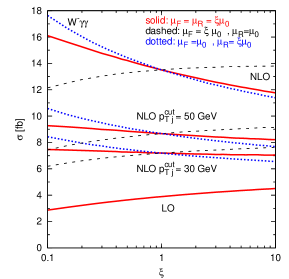
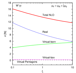
Figure 2: Left: Scale dependence of the total LHC cross section for $pp\to W^{-}\gamma\gamma+X\to\ell^{-}\gamma\gamma+p\hskip-5.03125pt\hbox to5.03125pt{\hss$/$\hss}_{T}+X$ at LO and NLO within the cuts of Eqs. (3.3, 3.4). The factorization and renormalization scales are together or independently varied in the range from $0.1\cdot\mu_{0}$ to $10\cdot\mu_{0}$. Right: Same as in the left panel but for the different NLO contributions at $\mu_{F}=\mu_{R}=\xi\mu_{0}$.

In Fig. 2 and Fig. 3, we show numerical results for $W^{-}\gamma\gamma$ production and $W^{+}\gamma\gamma$ production, respectively, within the cuts of Eqs. (3.3, 3.4). On the left panel of each figure, we show the overall scale variation of our numerical predictions at LO and NLO: as already shown in Table 2, the NLO K-factor is large both in absolute value ($\sim$ 3) and compared to the LO scale variation. The NLO scale uncertainty is about 10$\%$ when varying the factorization and the renormalization scale $\mu=\mu_{F}=\mu_{R}$ up and down by a factor 2 around the reference scale $\mu_{0}=m_{W\gamma\gamma}$ and is mainly driven by the dependence on $\mu_{R}$, which gives a negative slope with increasing energy, while the dependence on $\mu_{F}$ shows the opposite behaviour. In the left panels, we also show results for additional jet veto cuts, requiring $p_{Tj}<50$ GeV or $p_{Tj}<30$ GeV. From these curves, we can see that a large contribution to the total cross section is due to real jet radiation. While it is evident that the renormalization scale variation is highly reduced by a jet veto, this reduction should not be interpreted as a smaller uncertainty of the vetoed cross section: a similar effect in $WZj$ production could be traced to cancellations between different regions of phase space and, thus, the small variation is cut-dependent [21].

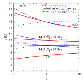
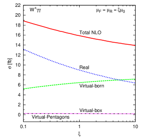
Figure 3: Same as Fig. 2, but for $pp\to W^{+}\gamma\gamma+X\to\ell^{+}\gamma\gamma+p\hskip-5.03125pt\hbox to5.03125pt{\hss$/$\hss}_{T}+X$ at the LHC.

Since the 1-jet contributions to the ${\cal O}(\alpha_{s})$ cross section are determined at LO only, their scale variation is large. In fact, most of the scale variation of the total NLO result is accounted for by the real emission contributions, defined here as the real emission cross section minus the Catani-Seymour subtraction terms plus the finite collinear terms. This is more visible in the right panels, where we show the scale dependence and compare the size of the different parts of the NLO calculation. As for the relative size of the NLO terms, the real emission contributions dominate and are even larger than the LO terms plus virtual terms proportional to the Born amplitude. Non-trivial virtual contributions, namely the interference of the Born amplitude with virtual-box and virtual-pentagon contributions, represent less than 1% of the total result and their scale dependence is basically flat.

3.3 Differential cross sections

Our numerical results show that the NLO corrections have a strong dependence on the phase space region under investigation. As a consequence, a simple rescaling of the LO results with a constant K-factor is not allowed. As practical examples, we plot several differential distributions at LO and NLO together with the associated K-factor, defined as

$$K=\frac{d\sigma^{NLO}/dx}{d\sigma^{LO}/dx}\,\,,$$ (3.6)

where $x$ denotes the considered observable. We usually show only one of the $W^{+}\gamma\gamma$ and $W^{-}\gamma\gamma$ distributions in the following since they share similar behaviors. Also, we include in all figures the results with an additional jet veto cut, requiring $p_{Tj}<50$ GeV.

In Fig. 4, we show the differential cross section as a function of the invariant mass of the photon pair, $M_{\gamma\gamma}$ for $W^{+}\gamma\gamma$ production. The corresponding K-factors lie between 2.5 and 3.5 in most of the phase space region.

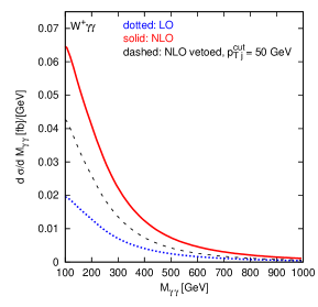
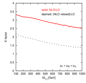
Figure 4: Left: Invariant mass distribution of the photon pair for $pp\to W^{+}\gamma\gamma+X\to\ell^{+}\gamma\gamma+p\hskip-5.03125pt\hbox to5.03125pt{\hss$/$\hss}_{T}+X$ production at the LHC. LO and NLO results are shown for $\mu_{F}=\mu_{R}=\mu_{0}$ and the cuts of Eqs. (3.3, 3.4). Right: K-factor as defined in Eq. (3.6).

In Fig. 5 (6), we show the transverse momentum distribution of the harder(softer) photon $p_{T\gamma,max}$($p_{T\gamma,min}$) in $W^{+}\gamma\gamma$ production. The K-factor is almost constant in the case of the harder photon $p_{T}$ distribution. For the $p_{T}$ distribution of the softer photon, we get the same large K-factor at low values of transverse momenta, but with a decrease of the NLO enhancement above $p_{T}\approx$ 50 GeV.

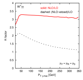
Figure 5: Left: Transverse-momentum distribution of the hardest photon in $pp\to W^{+}\gamma\gamma+X\to\ell^{+}\gamma\gamma+p\hskip-5.03125pt\hbox to5.03125pt{\hss$/$\hss}_{T}+X$ production at the LHC. LO and NLO results are shown for $\mu_{F}=\mu_{R}=\mu_{0}$ and the cuts of Eqs. (3.3, 3.4). Right: K-factor as defined in Eq. (3.6).

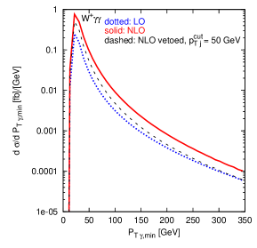
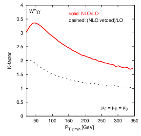
Figure 6: Left: Transverse-momentum distribution of the softest photon in $pp\to W^{+}\gamma\gamma+X\to\ell^{+}\gamma\gamma+p\hskip-5.03125pt\hbox to5.03125pt{\hss$/$\hss}_{T}+X$ production at the LHC. LO and NLO results are shown for $\mu_{F}=\mu_{R}=\mu_{0}$ and the cuts of Eqs. (3.3, 3.4). Right: K-factor as defined in Eq. (3.6).

Similar features emerge for distributions of the photon-lepton separations. In Fig. 7, the minimum of $R_{l\gamma_{1}}$ and $R_{l\gamma_{2}}$ is shown for $W^{-}\gamma\gamma$ production: the K-factor shows a large phase-space dependence and reaches values of 3 to 4 when the photons are emitted close to the lepton.

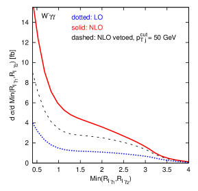
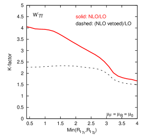
Figure 7: Left: Distribution of the minimum between $R_{l\gamma_{1}}$ and $R_{l\gamma_{2}}$ in $pp\to W^{-}\gamma\gamma+X\to\ell^{-}\gamma\gamma+p\hskip-5.03125pt\hbox to5.03125pt{\hss$/$\hss}_{T}+X$ production at the LHC. LO and NLO results are shown for $\mu_{F}=\mu_{R}=\mu_{0}$ and the cuts of Eqs. (3.3, 3.4). Right: K-factor as defined in Eq. (3.6).

Much larger values of the K-factor are possible in phase space regions which are difficult to access due to the LO kinematics. An example with a K-factor larger than 20 is shown in Fig. 8, where the transverse-momentum distribution of the lepton-photon-photon system is plotted. This large K-factor, indeed, is a feature shared by other triple vector boson production channels: the increase of the transverse-momentum of the observable electroweak system is compensated by a hard jet which appears first at NLO.

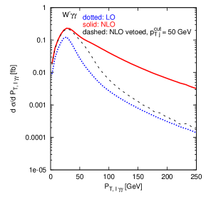
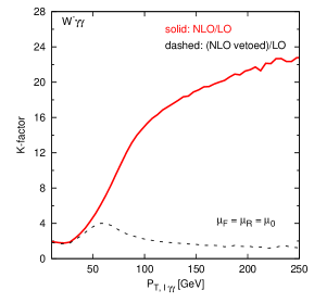
Figure 8: Left: Transverse-momentum distribution of the $\ell^{-}\gamma\gamma$ system in $pp\to W^{-}\gamma\gamma+X\to\ell^{-}\gamma\gamma+p\hskip-5.03125pt\hbox to5.03125pt{\hss$/$\hss}_{T}+X$ production at the LHC. LO and NLO results are shown for $\mu_{F}=\mu_{R}=\mu_{0}$ and the cuts of Eqs. (3.3, 3.4). Right: K-factor as defined in Eq. (3.6).

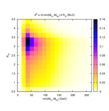
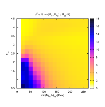
Figure 9: Left: Dependence of the NLO cross section on the couple of variables $(\min(M_{l\gamma_{1}},M_{l\gamma_{2}}),R_{\gamma_{1}\gamma_{2}})$. Same scales and cuts as in the previous diagrams. Right: K-factor as defined in Eq. (3.6).

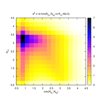
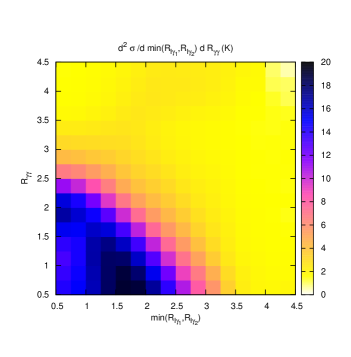
Figure 10: Left: Dependence of the NLO cross section on the couple of variables $(\min(R_{l\gamma_{1}},R_{l\gamma_{2}}),R_{\gamma_{1}\gamma_{2}})$. Same scales and cuts as in the previous diagrams. Right: K-factor as defined in Eq. (3.6).

Large K-factors also appear in the two-dimensional distributions of Figs. 9 and 10, where the dependence of the cross section on the pairs of variables $(\min(M_{l\gamma_{1}},M_{l\gamma_{2}}),R_{\gamma_{1}\gamma_{2}})$ and $(\min(R_{l\gamma_{1}},R_{l\gamma_{2}}),R_{\gamma_{1}\gamma_{2}})$, respectively, are shown, together with the corresponding K-factors. It is evident that very large NLO corrections arise particularly in regions where the lepton and photons are emitted close to each other and for low invariant masses of the lepton-photons system. However, since these regions contribute very little to the total cross section, this does not affect the overall K-factor, which is similar to the one observed in the bulk of the corrections in the differential distributions of Figs. 4 to 8. Note, however, that for the study of anomalous couplings, frequently extreme kinematics are selected. Therefore, large K-factors might appear.

3.4 Radiation Zero

As is known from the general theorem of Ref. [22], the SM amplitude for the process $q\bar{Q}\to W^{\pm}\gamma\gamma$ vanishes for $\cos\theta^{*}_{W}=\pm 1/3$ when the two photons are collinear. Here, $\theta^{*}_{W}$ denotes the angle between the incoming quark and the $W$ boson in the parton-center of mass frame. This radiation zero is not present in the gluon-induced channels, which enter in this process at NLO and are important at the LHC due to the steep rise of the gluon pdfs with smaller Feynman-x. The radiation zero only remains present when additional neutral (e.g. gluonic) radiation is collinear to the photon. Hence, additional QCD emission, as part of the NLO contribution to $W^{\pm}\gamma\gamma$ production, is expected to spoil the radiation zero, similar to the $W\gamma$ production process [23]. The resulting strong increase of the cross section near $\cos\theta^{*}_{W}=\pm 1/3$ can explain the large total K-factor for the $W^{\pm}\gamma\gamma$ process.

The radiation zero can be investigated, following Ref. [24], via rapidity difference distributions of the W and the photon pair system, $y_{\gamma\gamma}-y_{W}$, where $y_{W}$ is obtained from the $W$ momenta reconstructed out of the lepton and the missing transverse momentum. In our discussion we follow Ref. [7] and present results only for $W^{+}\gamma\gamma+X$ production since similar features are observed for $W^{-}\gamma\gamma+X$ production. The new element in the present discussion is that final state photon radiation (off the charged lepton) is included in the calculation.

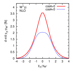
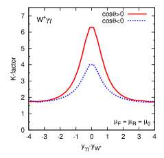
Figure 11: Distribution in rapidity separation between the W and the photon pair, with the photons in the same ($\cos\theta>0$) or opposite ($\cos\theta<0$) hemispheres, at LO (left), NLO (center) and K-factor (right).

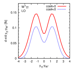
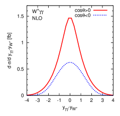
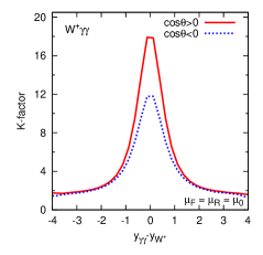
Figure 12: Same plots as in Fig. 11 with the additional cut on $M_{T,l\nu}>70$ GeV.

In Fig. 11, we plot the distribution in rapidity separation between the W and the photon pair, for photons lying in the same ($\cos\theta>0$) or opposite ($\cos\theta<0$) hemispheres in the laboratory frame. Our results at LO differ from the left-hand plot shown in Figure 3 of Ref. [7], where the W is considered as stable: our zero-rapidity dip for $\cos\theta<0$ is stronger than that for $\cos\theta>0$, while the opposite behaviour is observed in Ref. [7]. In both cases, the NLO corrections almost fill the dips, making an observation of a radiation zero at the LHC very difficult. In the K-factor plot of Fig. 11(c), the origin of the large total K-factor ($\sim$3) for $W^{\pm}\gamma\gamma$ production is clearly visible. This can be compared to other triple vector boson production processes with typical K-factor values between 1.5 and 2 [5, 1, 2, 6, 3, 4]. The suppression in the central region at LO due to the radiation zero is spoiled by the extra jet emission at NLO, giving rise to large K-factors in the bulk of the corrections and therefore large total K-factors. This is opposite to Figs. 8-10, where large K-factors appear in marginal phase space regions.

The difference observed at LO in Ref. [7] as compared to our results is due to the extra radiation of photons from the lepton line. In Fig. 12, we try to suppress this contribution by restricting the phase space for photon radiation in $W$ decay. Imposing a cut, $M_{T,l\nu}>70$ GeV, on the transverse mass of the charged lepton and neutrino, which is close to the kinematical limit for on-shell $W$s, strongly disfavors final state photon emission. This results in $y_{\gamma\gamma}-y_{W}$ distributions with a more pronounced dip for $\cos\theta>0$, in agreement with Ref. [7]. Note that even larger K-factors now appear in the central region, reaching values close to 20 in regions of large cross section.

For a better comparison with Reference [7], we also show our numerical results with an additional jet veto cut, $p_{Tj}<50$ GeV, in Fig. 13, with or without the cut on the invariant mass of the lepton-neutrino pair. Note also that, following Ref. [24], we use true rapidity and not pseudorapidity distributions, as was done in Ref. [7]. We have checked that our pseudorapidity plots, once we unphysically remove the extra radiation of the photon from the lepton line, are similar to those of Ref. [7]. It is interesting to see in the last plots, similar to Fig. 3 of Ref. [7], that once extra radiation is vetoed, a small dip is visible at NLO. This feature is particularly apparent in the right figure of Fig. 13, where final state photon radiation is also reduced. However, whether this dip should be interpreted as a sign of the radiation zero is questionable since it is more pronounced for photons in opposite hemispheres. As was pointed out in Ref. [25], ”signing” the quark direction according to overall boost of the event along the beam axis efficiently lifts the proton-proton initial state degeneracy at the LHC. Thereby, it reduces the distortion to the radiation zero by QCD activity and might aid in a more significant observation of the radiation zero. We have not investigated these questions in the present work.

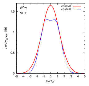
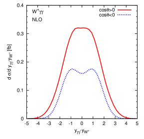
Figure 13: Left plot: NLO plot of Fig. 11 with the additional jet veto cut $p_{Tj}<50$ GeV. Right plot: NLO plot of Fig. 11 with the additional cuts $p_{Tj}<50$ GeV and $M_{T,l\nu}>70$ GeV.

4 Conclusions

We have calculated the NLO QCD corrections to the processes $pp,p\bar{p}\to$ $W^{\pm}\gamma\gamma$$+X$ with full leptonic and radiative decays of the $W$ boson. This process can be relevant as a background for New Physics searches and as a signal for the measurement of triple and quartic couplings at the LHC. It also represents an irreducible background to $WH$ production, when the Higgs boson decays into two photons.

Our numerical results show that this process gets very large corrections at NLO, even when compared to other triple boson production processes. The exceptionally large total K-factor is due to a cancellation between different diagrams at LO, leading to an approximate radiation zero, an effect which is spoiled by the extra jet emission at NLO. In certain regions of phase space the cross section increases by a factor of 20 with respect to the LO calculation. Apart from the vicinity of the radiation zero, this strong enhancement happens when the recoil against a hard jet at NLO is kinematically favorable. This latter effect was already observed in the NLO corrections to other triple boson production processes. However, these high transverse momentum effects do not significantly contribute to the bulk of the cross section corrections and do not affect the total K-factor. Nevertheless, for the study of anomalous couplings, extreme kinematics are typically selected. Therefore, large K-factors might appear and the NLO corrections have to be taken into account.

$W^{\pm}\gamma\gamma$  production at the LHC provides an additional example of a cross section whose theoretical errors at LO are substantially underestimated by considering scale variations only: the LO factorization scale variation is much smaller than the size of NLO corrections. Remaining NLO scale variations are at the 10% level for the integrated $W^{\pm}\gamma\gamma$  production cross section at the LHC when varying $\mu_{R}=\mu_{F}=\mu_{0}$ by a factor of 2 around the reference scale $\mu_{0}=m_{WW\gamma}$.

Given the size of the higher-order corrections and, in particular, their strong dependence on the observable and on different phase space regions under investigation, a fully-flexible NLO parton Monte Carlo for $W^{\pm}\gamma\gamma$  production is required to match the expected precision of the LHC measurements. We plan to incorporate this and other processes with a final state photon into the VBFNLO  package in the near future.

References

- [1] V. Hankele and D. Zeppenfeld, Phys. Lett. B 661 (2008) 103 [arXiv:0712.3544 [hep-ph]].
- [2] F. Campanario, V. Hankele, C. Oleari, S. Prestel and D. Zeppenfeld, Phys. Rev. D 78 (2008) 094012 [arXiv:0809.0790 [hep-ph]].
- [3] G. Bozzi, F. Campanario, V. Hankele and D. Zeppenfeld, Phys. Rev. D 81 (2010) 094030 [arXiv:0911.0438 [hep-ph]].
- [4] G. Bozzi, F. Campanario, M. Rauch, H. Rzehak and D. Zeppenfeld, Phys. Lett. B 696, 4 (2011) arXiv:1011.2206 [hep-ph].
- [5] A. Lazopoulos, K. Melnikov and F. Petriello, Phys. Rev. D 76 (2007) 014001 [arXiv:hep-ph/0703273].
- [6] T. Binoth, G. Ossola, C. G. Papadopoulos and R. Pittau, JHEP 0806 (2008) 082 [arXiv:0804.0350 [hep-ph]].
- [7] U. Baur, D. Wackeroth and M. M. Weber, PoS RADCOR2009, 067 (2010) [arXiv:1001.2688 [hep-ph]].
- [8] S. Godfrey, arXiv:hep-ph/9505252; P. J. Dervan, A. Signer, W. J. Stirling and A. Werthenbach, J. Phys. G 26 (2000) 607 [arXiv:hep-ph/0002175]; O. J. P. Eboli, M. C. Gonzalez-Garcia, S. M. Lietti and S. F. Novaes, Phys. Rev. D 63 (2001) 075008 [arXiv:hep-ph/0009262]; P. J. Bell, arXiv:0907.5299 [hep-ph].
- [9] J. M. Campbell, J. W. Huston and W. J. Stirling, Rept. Prog. Phys. 70, 89 (2007) [arXiv:hep-ph/0611148].
- [10] CMS Collaboration, CMS-PAS-SUS-09-004, (2009).
- [11] S. Frixione, Phys. Lett. B 429, 369 (1998) [arXiv:hep-ph/9801442].
- [12] K. Arnold et al., Comput. Phys. Commun. 180 (2009) 1661 [arXiv:0811.4559 [hep-ph]].
- [13] B. Jager, C. Oleari and D. Zeppenfeld, JHEP 0607 (2006) 015 [arXiv:hep-ph/0603177]; B. Jager, C. Oleari and D. Zeppenfeld, Phys. Rev. D 73, 113006 (2006) [arXiv:hep-ph/0604200]; G. Bozzi, B. Jager, C. Oleari and D. Zeppenfeld, Phys. Rev. D 75 (2007) 073004 [arXiv:hep-ph/0701105].
- [14] K. Hagiwara and D. Zeppenfeld, Nucl. Phys. B 274 (1986) 1; K. Hagiwara and D. Zeppenfeld, Nucl. Phys. B 313 (1989) 560.
- [15] S. Catani and M. H. Seymour, Nucl. Phys. B 485 (1997) 291 [Erratum-ibid. B 510 (1998) 503] [arXiv:hep-ph/9605323].
- [16] A. Denner and S. Dittmaier, Nucl. Phys. B 658, 175 (2003) [arXiv:hep-ph/0212259]; A. Denner and S. Dittmaier, Nucl. Phys. B 734, 62 (2006) [arXiv:hep-ph/0509141].
- [17] T. Stelzer and W. F. Long, Comput. Phys. Commun. 81 (1994) 357 [arXiv:hep-ph/9401258]; F. Maltoni and T. Stelzer, JHEP 0302 (2003) 027 [arXiv:hep-ph/0208156].
- [18] T. Gleisberg, S. Hoche, F. Krauss, M. Schonherr, S. Schumann, F. Siegert and J. Winter JHEP 02 (2009) 007
- [19] J. Pumplin, D. R. Stump, J. Huston, H. L. Lai, P. Nadolsky and W. K. Tung, JHEP 0207 (2002) 012 [arXiv:hep-ph/0201195].
- [20] H. -L. Lai, M. Guzzi, J. Huston et al., Phys. Rev. D82 (2010) 074024. [arXiv:1007.2241 [hep-ph]].
- [21] F. Campanario, C. Englert, S. Kallweit, M. Spannowsky and D. Zeppenfeld, JHEP 1007 (2010) 076 [arXiv:1006.0390 [hep-ph]].
- [22] R. W. Brown, K. L. Kowalski, S. J. Brodsky, Phys. Rev. D28 (1983) 624.
- [23] U. Baur, T. Han, J. Ohnemus, Phys. Rev. D48 (1993) 5140-5161. [hep-ph/9305314].
- [24] U. Baur, T. Han, N. Kauer, R. Sobey, D. Zeppenfeld, Phys. Rev. D56 (1997) 140-150. [hep-ph/9702364].
- [25] M. Dobbs, AIP Conf. Proc. 753 (2005) 181-192. [hep-ph/0506174].
- [26] J. A. M. Vermaseren, Comput. Phys. Commun. 83 (1994) 45.