Theoretical Properties of the Overlapping Groups Lasso

Abstract

We present two sets of theoretical results on the grouped lasso with overlap due to Jacob, Obozinski and Vert (2009) in the linear regression setting. This method jointly selects predictors in sparse regression, allowing for complex structured sparsity over the predictors encoded as a set of groups. This flexible framework suggests that arbitrarily complex structures can be encoded with an intricate set of groups. Our results show that this strategy results in unexpected theoretical consequences for the procedure. In particular, we give two sets of results: (1) finite sample bounds on prediction and estimation, and (2) asymptotic distribution and selection. Both sets of results demonstrate negative consequences from choosing an increasingly complex set of groups for the procedure, as well for when the set of groups cannot recover the true sparsity pattern. Additionally, these results demonstrate the differences and similarities between the the grouped lasso procedure with and without overlapping groups. Our analysis shows that while the procedure enjoys advantages over the standard lasso, the set of groups must be chosen with caution — an overly complex set of groups will damage the analysis.

t1This work is part of the author’s Ph.D thesis. t2This work was funded by the National Institutes of Health grant MH057881 and National Science Foundation grant DMS-0943577. The author was also partially supported by National Institutes of Health SBIR grant 7R44GM074313-04 at Insilicos LLC. t3The author would like to thank Larry Wasserman and Aarti Singh for helpful comments and discussions, as well as the two anonymous referees whose suggestions helped greatly improve the contents of this paper.

1 Introduction

In this paper, we consider the linear regression model: $\textbf{y}=\textbf{X}\beta^{0}+{\epsilon}$, where X is an $n\times p$ real valued data matrix, $\textbf{y}\in\mathbb{R}^{n}$ is a vector of responses, $\beta^{0}\in\mathbb{R}^{p}$ is a vector of linear weights, and ${\epsilon}$ is an error vector. Much work focuses on estimating a sparse $\widehat{\beta}$, where many of the entries are equal to zero, effectively excluding many of the dimensions of X — the candidate predictors — from the model. Recent work adds the notion of structure to this setting. That is, we desire the set of nonzero entries in $\widehat{\beta}$ to follow some predefined structure over the candidate predictors. There are now many methods tailored to a diverse collection of structures, including hierarchical structures, group structures, and graph derived structures: see Bach (2010a, 2008b, b); Huang, Zhang and Metaxas (2009); Jenatton, Audibert and Bach (2009); Jenatton, Obozinski and Bach (2010); Peng et al. (2010); Percival et al. (2011); Kim and Xing (2010); Zhao et al. (2007) for examples.

One such structured sparse method is the grouped lasso of Yuan et al. (2006), which extends the familiar $\ell_{1}$ penalization to a grouped $\ell_{1}$ norm. In particular, the grouped lasso allows for groups of predictors to enter the model together, a useful property in settings such as ANOVA or multi-task regression. For example, we can encode a factor predictor with $m$ levels as $m-1$ indicator variables in X. When we build a sparse regression model, we might prefer to select none or all of this group of $m-1$ variables, but not any other subset. The grouped lasso enables this type of grouped selection. Bach (2008a); Chesneau and Hebiri (2008); Huang and Zhang (2010); Lounici et al. (2009); Nardi and Rinaldo (2008) give theoretical results for this procedure, including oracle inequalities and asymptotic distributions. In particular, they showed that for some problems the grouped lasso outperforms the ordinary lasso.

However, the grouped $\ell_{1}$ norm of the grouped lasso is limited in that it only allows groups that partition the set of candidate predictors. This restricts the complexity and types of structures over the candidate predictors that can be encoded in the groups. For example, we could represent the potential structures of $\beta^{0}$ as a a graph over $p$ nodes, where each node represents a candidate predictor. We might then seek to build a sparse model where the selected predictors correspond to a subgraph, such as a neighborhood or clique, of this graph. This structure can be encoded, for example, as a series of overlapping neighborhoods, such as 4-cycles in a 2-dimensional lattice graph. The grouped $\ell_{1}$ norm does not allow for such a set of groups.

The grouped lasso with overlap of Jacob, Obozinski and Vert (2009) is one solution to this problem (see also the CAP penalty of Zhao et al. (2007), as well as other group based procedures in Bach (2010b); Jenatton, Audibert and Bach (2009)). Using an extension of the grouped norm of the grouped lasso, this procedure allows for complex, overlapping group structures. Given a collection of subsets of the set of candidate predictors, the procedure recovers nonzero patterns equal to a union of some subset of this collection. This property can encode many complex structures over the candidate predictors, and thus within the resulting sparsity patterns of the estimated coefficients. While Jacob, Obozinski and Vert (2009) gave some initial theoretical results on this procedure, including a consistency result, many theoretical questions were left open. In particular, the impact on the predictive and estimation performance of the procedure of increasingly complex sets of groups remained unanswered. The overlapping nature of the groups allows the possibility for an arbitrarily large set of groups to encode complex structures, or many possible structures simultaneously. If we suppose that there is no consequence to increasing the number and complexity of the groups, then we can freely run the procedure under many structural conditions simultaneously.

The concluding remarks of Huang and Zhang (2010) indicate that the grouped lasso does not perform well with overlapping groups. The goal of this paper is to expose exactly how introducing the possibility of overlapping groups impacts the grouped lasso. Towards this goal, we demonstrate some theoretical properties of the overlapping grouped lasso, with a focus on the consequence of the number and complexity of the groups of predictors. We give a finite sample and an asymptotic result. In particular, we make the following contributions:

1. We show that both the finite sample and asymptotic performance of the overlapping grouped lasso suffers as the number and complexity of the groups grows.

2. In the finite sample case, we show that the assumptions on the design matrix X become more restrictive as the complexity of the groups grows.

3. In our asymptotic analysis, we introduce the adaptive overlapping grouped lasso, and give an adaptive weighting scheme with asymptotic selection guarantees similar to the adaptive lasso of Zou (2006) (see also the adaptive grouped lasso results in Nardi and Rinaldo (2008)).

Overall, we conclude that the overlapping grouped lasso enjoys many of the same theoretical guarantees as the grouped lasso, provided that the set of groups are not too complex or large. We therefore recommend that the procedure should be used with a set of groups that is not overly complex, or contains a nested structure.

The paper is organized as follows: we first introduce notation for the overlapping grouped lasso. We also reproduce some basic theoretical properties of the procedure and the associated overlapping grouped norm. We next give our finite sample results, and then our asymptotic results. We then present a simulation study to support our theoretical results. Proofs of the main results along with supporting lemmas appear in the appendix.

2 Notation

We adopt a combination of the notation of Jacob, Obozinski and Vert (2009) and Lounici et al. (2009). Recall our basic setting, the linear model:

$$\textbf{y}=\textbf{X}\beta^{0}+\epsilon.$$ (1)

Here, X is an $n\times p$ data matrix, $\textbf{y}\in\mathbb{R}^{n}$ is the response, $\beta^{0}\in\mathbb{R}^{p}$ is a vector of true linear coefficients, and $\epsilon$ is a stochastic error term. Our goal is to estimate a sparse $\widehat{\beta}$, such that the nonzero entries follow some structure which we assume to be known a priori. In particular, we consider structures defined in terms of groups of predictors, which we define as subsets of the set of candidate predictors indices: $\mathcal{I}=\{1,2,\ldots,p\}$. We denote a collection of groups as $\mathcal{G}$ with elements $g$ such that each $g\subseteq\mathcal{I}$. Let $|\mathcal{G}|=M$, and assume $\displaystyle\bigcup_{g\in\mathcal{G}}g=\mathcal{I}$. For coefficient vectors $\beta$, we define $\beta_{g}\in\mathbb{R}^{|g|}$ as the sub vector consisting of the entires corresponding to the indices in $g$. Define the support of a vector as:

$$\mbox{supp}(\beta)=\{i:\beta_{i}\neq 0\}\subseteq\mathcal{I}.$$ (2)

We now give a framework, proposed by Jacob, Obozinski and Vert (2009), to measure the structured sparsity of vectors in $\mathbb{R}^{p}$. We define the following convention: for vectors denoted $v_{g}\in\mathbb{R}^{p}$ we have that $\mbox{supp}(v_{g})\subseteq g$. We define a decomposition of $\beta\in\mathbb{R}^{p}$ with respect to $\mathcal{G}$ as:

$$\mathcal{V}_{\mathcal{G}}(\beta)=\left\{v_{g}:g\in\mathcal{G}\right\}\mbox{ such that }\sum_{g\in\mathcal{G}}v_{g}=\beta.$$ (3)

That is, each decomposition in $\mathcal{V}_{\mathcal{G}}(\beta)$ is a collection of $M$ vectors in $\mathbb{R}^{p}$ each satisfying $\mbox{supp}(v_{g})\subseteq g$ for a different $g\in\mathcal{G}$. From now on, we suppress the $\mathcal{G}$ in the notation for decompositions and write $\mathcal{V}(\beta)$. $\mathcal{V}(\beta)$ is not unique in general. We define the following norms:

$$||\beta||_{2,p,\mathcal{G}} =\min_{\mathcal{V}(\beta)}\left(\sum_{g\in\mathcal{G}}\left(\sum_{i\in g}v_{g,i}^{2}\right)^{p/2}\right)^{1/p},$$ (4)

$$=\min_{\mathcal{V}(\beta)}\left(\sum_{g\in\mathcal{G}}||v_{g}||^{p}\right)^{1/p};$$ (5)

$$||\beta||_{2,\infty,\mathcal{G}} =\min_{\mathcal{V}(\beta)}\max_{g\in\mathcal{G}}||v_{g}||.$$ (6)

Here, $||\cdot||$ denotes the Euclidean or $\ell_{2}$ norm. The above two equations are norms by arguments presented in Jacob, Obozinski and Vert (2009). Note that the notation $\min_{\mathcal{V}(\beta)}$ indicates the minimum over all possible decompositions. Note that the decomposition that minimizes these norms is not necessarily unique, as we state in the following lemma.

Lemma 1.

(Corollary 1 from Jacob, Obozinski and Vert (2009)) For any collections $\{v_{g}\}$, $\{v_{g}^{\prime}\}$ minimizing the norm 5, we have, $\forall g\in\mathcal{G}$:

$$||v_{g}||\times||v_{g}^{\prime}||=0\mbox{ or }\frac{v_{g}}{||v_{g}||}=\frac{v_{g}^{\prime}}{||v_{g}^{\prime}||}.$$ (7)

The above lemma implies that in some cases the collection of groups used in the decomposition — that is, $\{g\in\mathcal{G}\mbox{ s.t. }v_{g}\neq 0$} — is not unique.

Finally, for $J\subset\mathcal{G}$ we write $\beta_{J}=\sum_{g\in G}v_{g}1_{g\in J}$, note that $J\subseteq\{1,2,\ldots,M\}$. Let $J_{v}(\beta)=\{g:v_{g}\neq 0\}$, and $M_{v}(\beta)=|J_{v}(\beta)|$. Thus, $J_{v}(\beta)$ is the set of groups used to decompose $\beta$ for a particular decomposition. $M_{v}(\beta)$ is thus a measure of the structured sparsity of $\beta$ with respect to a particular decomposition. Let $M(\beta)=\min_{v}M_{v}(\beta)$, where this minimum is taken over the set of decompositions minimizing the norm 5. Thus, $M(\beta)$ measures the overall structured sparsity of $\beta$, with respect to the groups $\mathcal{G}$.

Here is a simple example to illustrate the setting. Let $p=3$, and consider the following groups:

$$\mathcal{G}=\{\{1,2\},\{2,3\}\}.$$ (8)

For any $\alpha\in\mathbb{R}$, we have the following possible decomposition of $\beta=[a,b,c]$:

$$\mathcal{V}(\beta) =\{v_{\{1,2\}},v_{\{2,3\}}\},$$ (9)

$$v_{\{1,2\}} =[a,\alpha b,0],$$ (10)

$$v_{\{2,3\}} =[0,(1-\alpha)b,c].$$ (11)

Thus, the norm from Equation 5 can be expressed as:

$$||\beta||_{2,1,\mathcal{G}}=\min_{\alpha}\left(\sqrt{a^{2}+(\alpha b)^{2}}+\sqrt{((1-\alpha)b)^{2}+c^{2}}\right).$$ (12)

Finally, it is clear that for $a,c\neq 0$, $M(\beta)=2$, and $M(\beta)=1$ otherwise.

3 Overlapping Grouped Lasso

Recall our goal, under the model of Equation 1, we estimate the target $\beta^{0}$ with a sparse $\widehat{\beta}$ – that is, many entires of $\widehat{\beta}$ are set to zero. Additionally, we know these nonzero entries occur in a structured pattern, as given by $\mathcal{G}$. We evaluate the fit with the usual quadratic loss:

$$\ell(\beta) =\frac{1}{n}||\textbf{y}-\textbf{X}\beta||^{2}.$$ (13)

The overlapping grouped lasso solves the following optimization problem:

$$\widehat{\beta}=\underset{\boldsymbol{\beta}\in\mathbb{R}^{p}}{\operatorname{argmin}}\left(\ell(\beta)+2\lambda||\beta||_{2,1,\mathcal{G}}\right).$$ (14)

Here $\lambda>0$ is a tuning parameter controlling the amount of regularization. If the elements of $\mathcal{G}$ are restricted to be pairwise disjoint, then the norm $||\cdot||_{2,1,\mathcal{G}}$ reduces to the grouped $\ell_{1}$ norm. We then recover the original formulation of the grouped lasso. In the special case where the groups are all singletons: $\mathcal{G}=\{\{i\}:i\in\mathcal{I}\}$, we recover the familiar lasso Tibshirani (1996). If we allow $\mathcal{G}$ to be any collection, allowing for the possibility of overlap between groups, then the minimum over $\mathcal{V}(\beta)$ in the norm now plays a role since the decomposition of $\beta$ is no longer unique in general. This setting gives us the overlapping grouped lasso. For each of these problems, the key fact is that the support of $\widehat{\beta}$ will be a union of members of a subset of $\mathcal{G}$. Finally, we also introduce the the adaptive overlapping grouped lasso:

$$\widehat{\beta}=\underset{\boldsymbol{\beta}\in\mathbb{R}^{p}}{\operatorname{argmin}}\left({\ell}(\beta)+2\lambda\min_{\mathcal{V}(\beta)}\sum_{g\in\mathcal{G}}\lambda_{g}||v_{g}||\right).$$ (15)

As previous work and theory has suggested (Nardi and Rinaldo (2008); Zou (2006)), the choice of weights: $\lambda_{g}=1/||\beta^{{OLS}}_{g}||^{\gamma}$, where $\beta^{OLS}=(\textbf{X}^{T}\textbf{X})^{-1}\textbf{X}^{T}\textbf{y}$, and $\gamma>0$, gives good asymptotic guarantees. In Section 5, we show that a different choice is needed in our setting to give similar asymptotic guarantees.

Finally, as noted by Jacob, Obozinski and Vert (2009), the overlapping grouped lasso method is simple to implement. In the case where $\mathcal{G}$ consists of non-overlapping groups, there are several efficient algorithms available. In the overlapping case, no new specialized algorithm is required. Write $\textbf{X}_{g}$ as the sub-matrix of X with only the columns of X indexed by the elements of $g$. Now define $\widetilde{\textbf{X}}=[\textbf{X}_{g}]_{g\in\mathcal{G}}$ — a $n\times\sum_{g}|g|$ matrix of the concatenation of the columns of X corresponding to each group in $\mathcal{G}$. We then can solve the optimization problem with with a new, non-overlapping, set of groups $\mathcal{G}$ defined on the appropriate columns of $\widetilde{\textbf{X}}$. Since $\mathcal{G}$ is now a non-overlapping set of groups for $\widetilde{\textbf{X}}$, we can simply apply existing algorithms for the grouped lasso.

4 Finite Sample Bounds

We now give a sparsity oracle inequality for the overlapping grouped lasso. This finite sample result is an extension of a result on multitask regression due to Lounici et al. (2009), which is in turn built on results from Bickel, Ritov and Tsybakov (2009). We first state and discuss our main assumption, which is an adaptation of the restricted eigenvalue condition of Bickel, Ritov and Tsybakov (2009) to the overlapping grouped lasso seetting.

Assumption 1.

Suppose $1\leq s\leq M=|\mathcal{G}|$. Then there exists $\kappa(s)>0$ such that:

$$\kappa(s) \leq\min\left\{\frac{\sqrt{\Delta^{T}X^{T}X\Delta}}{\sqrt{n}\sum_{g\in J}||v_{g}^{\Delta}||}:J\subseteq\mathcal{G};J\in\mathcal{J}(s)\right\},$$ (16)

$$\mathcal{J}(s) :=\left\{J\subseteq\mathcal{G};|J|\leq s;\Delta\in\mathbb{R}^{p}\backslash\textbf{0};\ \mathcal{V}(\Delta)=\{v_{g}^{\Delta}\}\mbox{ s.t. }\sum_{g\in J^{c}}||v_{g}^{\Delta}||\leq 3\sum_{g\in J}||v_{g}^{\Delta}||\right\}.$$ (17)

Here $J^{c}=\{g:g\in\mathcal{G},g\notin J\}$, and $\mathcal{V}(\Delta)=\{v_{g}^{\Delta}\}$ denotes the decomposition minimizing the norm $||\Delta||_{2,1,\mathcal{G}}$.

In the subsequent results, the integer $s$ measures the structured sparsity of the target. There are two key differences between this assumption and other restricted eigenvalue conditions. First, it relies on norms of the decompositions of vectors, rather than norms of the vector or appropriate sub-vectors. Note that the decomposition of $\Delta$ must be a decomposition minimizing the $||\cdot||_{2,1,\mathcal{G}}$ norm. As we will discuss later, this condition grows more restrictive as $\mathcal{G}$ becomes more complex. The key second difference in the assumption lies in the denominator term $\sum_{g\in J}||v_{g}^{\Delta}||$, which appears instead of the directly analogous $||\sum_{g\in J}v_{g}^{\Delta}||$. We know by the triangle inequality that $||\sum_{g\in J}v_{g}^{\Delta}||\leq\sum_{g\in J}||v_{g}^{\Delta}||$, and so our $\kappa$ is less than or equal to a $\kappa^{\prime}$ obtained under the analogous assumption. In the case of non-overlapping groups, this is an equality, and the assumption is identical in this case.

We now examine some sufficient conditions for the existence of $\kappa(s)$. Examining the numerator of the main quantity defining $\kappa(s)$, we see that $\sqrt{\Delta^{T}X^{T}X\Delta/n}\geq|\rho_{X}|^{1/2}||\Delta||$, where $\rho_{X}$ is the minimal eigenvalue of $X^{T}X/n$. Examining the denominator, we can make the following bounds:

$$\sum_{g\in J}||v_{g}^{\Delta}|| \leq\sum_{g\in\mathcal{G}}||v_{g}^{\Delta}||$$ (18)

$$\leq\sum_{g\in\mathcal{G}}||\Delta_{g}||$$ (19)

$$\leq||\Delta||(M\mathcal{G}_{\mbox{overlap}})^{1/2}.$$ (20)

Here, $\mathcal{G}_{\mbox{overlap}}:=\max_{j\in\mathcal{I}}\left[\sum_{g\in\mathcal{G}}1_{j\in g}\right]$ is the maximal number of times a candidate predictor appears in the groups of the collection $\mathcal{G}$. Thus, as long as $X^{T}X$ has a nonzero minimal eigenvalue, we are guaranteed to find a $\kappa(s)$ of at most $(\rho_{X}/M\mathcal{G}_{\mbox{overlap}})^{1/2}$. In particular, for $\kappa(s)$ to exist, it is sufficient for $X^{T}X$ to be positive definite. We now state our main result.

Theorem 1.

Consider the model in Equation 1. Suppose $|\mathcal{G}|=M\geq 2$, and $n\geq 1$. Assume that the entries of $\epsilon$ are i.i.d. Gaussian with mean 0 and variance $\sigma^{2}$. Let X be normalized so that the the diagonal entries of $\textbf{X}^{T}\textbf{X}/n$ are all equal to 1. Denote $M(\beta^{0})\leq s$ as the maximum number of nonzero groups in decompositions of $\beta^{0}$, $\mathcal{V}(\beta^{0})$. Let Assumption 1 hold with $\kappa=\kappa(s)$. Let:

$$\lambda=\frac{2\sigma\sqrt{\max_{g}|g|\mathcal{G}_{\mbox{overlap}}}}{\sqrt{n}}\left(1+\frac{A\log M}{\sqrt{\max_{g}|g|}}\right)^{1/2}.$$ (21)

Here, $A>8$. Define $q=\min_{g}(\rho_{g}^{-2})\min\left(A\sqrt{\min_{g}|g|}/8,8\log M\right)$, where $\rho_{g}$ is the maximal absolute eigenvalue of a Cholesky decomposition of $\textbf{X}_{g}^{T}\textbf{X}_{g}$, where $\textbf{X}_{g}$ is the sub matrix of X corresponding to the columns indexed by the group $g$. Then, with probability at least $1-M^{1-q}$, for any solution $\widehat{\beta}$ to Equation 14, for all $\beta^{0}\in\mathbb{R}^{p}$, the following inequalities hold:

$$\frac{1}{n}||X(\widehat{\beta}-\beta^{0})||^{2} \leq\frac{64\sigma^{2}}{\kappa^{2}n}\left(\max_{g}|g|+A\sqrt{\max_{g}|g|}\log M\right),$$ (22)

$$||\widehat{\beta}-\beta^{0}||_{2,1,\mathcal{G}} \leq\frac{32\sigma}{\kappa\sqrt{n}}\left(\max_{g}|g|+A\sqrt{\max_{g}|g|}\log M\right)^{1/2}.$$ (23)

The proof for this result is given in the appendix A.1.2. The proof relies on Lemma 4 given in the appendix A.1.1. We now discuss the result.

1. As the set of groups grows, the finite sample guarantees degrade. In Proposition 1, the prediction and estimation bounds both get coarser as the number of groups increases. Note that the set of groups can grow not only as the dimension of the problem grows, but also if we encode complex structures over the predictors using $\mathcal{G}$. Thus, even for a problem of fixed dimension $p$, there is a consequence to choosing an arbitrarily complex set of groups. To make this result clear, let the groups be maximally complex: $\mathcal{G}=2^{\mathcal{I}}$, the power set of the set of predictors. Now, as the dimension of the problem grows, the prediction bound grows at rate $O(p^{3/2})$, and the estimation bound at rate $O(p)$. If $|\mathcal{G}|$ is instead of the same order as $p$ and the maximum group size is constant, these rates are instead both $O(\log p)$. This shows that grouped sparsity achieves the tightest upper bounds if both the maximum group size and the number of groups grow at slower rates than $p$. Note the contrast here to the results of Lounici et al. (2009) in the multi-task setting, where a growing number of tasks benefitted the procedure. Note that in multi-task setting, the number of observations necessarily grows with the number of tasks, contrary to our setting.

2. As the complexity of the groups grows, Assumption 1 becomes more restrictive. Since $\kappa$ appears in the denominator of both the prediction and estimation bounds, the bounds become less tight as $\kappa$ decreases. Consider the condition:

   $$\sum_{g\in J^{c}}||v_{g}^{\Delta}||\leq 3\sum_{g\in J}||v_{g}^{\Delta}||.$$ (24)

   Recall that $J$ is a cardinality $s$ set of groups. Thus, for fixed $s$, as the complexity of $\mathcal{G}$ grows, the flexibility of the decompositions grows, and then more vectors $\Delta$ satisfy this condition. This makes $\kappa$ decreasing as a function of $|\mathcal{G}|$. We also recall that when $X^{T}X$ has a nonzero minimal absolute eigenvalue, we know $\kappa$ is at most $\sqrt{\rho_{X}/M\mathcal{G}_{\mbox{overlap}}}$. As noted earlier, as the complexity of the groups grows, $\mathcal{G}_{\mbox{overlap}}$ increases as well, leading to a smaller $\kappa$ and in turn inferior prediction and estimation bounds. If $\mathcal{G}_{\mbox{overlap}}$ is on the same order as the number of predictors, then $\kappa(s)$ is of order $1/M$ rather than $1/\sqrt{M}$. This dependence shows that our bounds depend equally on the dimension of the problem $M$ and the group complexity as measured by $\mathcal{G}_{\mbox{overlap}}$. In the case of the lasso or group lasso, $\mathcal{G}_{\mbox{overlap}}=1$, giving us no dependence on group complexity, as expected.

3. The results show that the procedure enjoys an advantage over non-structured procedures when $\beta^{0}$ is structured sparse. For example, in the finite sample case, none of our bounds depended explicitly on the dimension of the problem $p$. Thus, we can adopt a similar argument to those of Lounici et al. (2009) to show that compared to the lasso, the overlapping grouped lasso gives superior results in the case where $\beta^{0}$ is structured sparse. That is, from Bickel, Ritov and Tsybakov (2009), if we let:

   $$\lambda=A\sigma\sqrt{\frac{\log p}{n}},$$ (25)

   then for $A>2\sqrt{2}$, we have that with probability at least $1-(p)^{1-A^{2}/8}$:

   $$\frac{1}{n}||X(\widehat{\beta}_{\mbox{lasso}}-\beta^{0})||^{2}\leq\frac{16A^{2}\sigma^{2}}{\kappa^{2}n}\log p.$$ (26)

   Thus, if $\sqrt{\max_{g}|g|}\log M+\max_{g}|g|$ is of smaller order than $\log p$, the procedure has a predictive advantage. Since $\kappa$ depends on the structured sparsity of the target, this result holds only for structured sparse targets $\beta^{0}$ which give sufficiently large values of $\kappa$ under our assumption.

4. In the non-overlapping case, we can recover many results available in the literature. Here we have $\mathcal{G}_{\mbox{overlap}}=1$. We adjust our assumption to match the literature, so that the quantity in the minimum is replaced with:

   $$\frac{\sqrt{\Delta^{T}X^{T}X\Delta}}{\sqrt{n}\left|\left|\sum_{g\in J}v_{g}^{\Delta}\right|\right|}.$$ (27)

   Combining this with an application of the Cauchy-Schwarz inequality in the last steps of the proofs of the result, we can recover the results of Lounici et al. (2009) in the multi-task case. In the case of the grouped lasso, we can recover the result from Nardi and Rinaldo (2008). The dependence on the minimal eigenvalues of the Cholesky decomposition of each $\textbf{X}_{g}^{T}\textbf{X}_{g}$ is related to the conditions given in Huang and Zhang (2010). In the settings of Lounici et al. (2009), $\rho_{g}=1$ for all $g$.

5. We can show a similar result solely in terms of $\max_{g}|g|$. In particular, for:

   $$\lambda=\frac{2\sigma\sqrt{\mathcal{G}_{\mbox{overlap}}}}{\sqrt{n}}\left(\max_{g}|g|+A\log M\right)^{1/2},$$ (28)

   the same results hold with probability $1-M^{1-q}$, for $q=\min_{g}(\rho_{g}^{-2})\min\left(A/8,\frac{8\log M}{\max_{g}|g|}\right)$. This result is a consequence of a simple adjustment for this choice of $\lambda$ in the proof of Lemma 4 from the appendix. This alternate result shows that as the maximum group size grows, the estimation and prediction bounds become less tight, and the probability that they hold falls.

6. The result does not depend on the any uniqueness assumptions on the decomposition of $\beta^{0}$. The consistency result for the overlapping grouped lasso in Jacob, Obozinski and Vert (2009) assumes that the decomposition of $\beta^{0}$ that minimizes the $||\cdot||_{2,1,\mathcal{G}}$ norm is unique. Our result, in contrast, depends only on the maximal structured sparsity of such decompositions. Thus, in the case where $\beta^{0}$ does not have a unique decomposition minimizing the $||\cdot||_{2,1,\mathcal{G}}$ norm, our results still hold. This is a contrast to the asymptotic results of the next section.

5 Asymptotic Results

In this section, we consider fixed dimension asymptotic for the adaptive overlapping grouped lasso as described in Equation 15. These results extend those on the grouped lasso found in Nardi and Rinaldo (2008) to the case of overlapping groups.

To begin, define the set of indices of the true linear coefficient vector $\beta^{0}$ which are nonzero and zero as the following:

$$H =\{i:\beta^{0}_{i}\neq 0\},$$ (29)

$$H^{c} =\{i:\beta^{0}_{i}=0\}.$$ (30)

Accordingly, we define $\textbf{X}_{H}$ as the sub matrix containing the entries with column indices in the set $H$. Similarly, for a $p$-vector $x$, let $x_{H}$ be the sub vector containing the entries with indices in the set $H$. Clearly, $H\cup H^{c}=\mathcal{I}$. However, that $H$ and $H^{c}$ are not necessarily the union of members of $J(\beta^{0})$ and $J(\beta^{0})^{c}$, respectively. We next define the following three subsets of $\mathcal{G}$ related to $H$ and $H^{c}$:

$$G_{H}= \{g:g\subseteq H\},$$ (31)

$$G_{Hc}= \{g:g\subseteq H^{c}\},$$ (32)

$$G_{Ho}= \{g:|g\cap H|>0;|g\cap H^{c}|>0\}.$$ (33)

These are, respectively, the set of groups in which the indices are all nonzero in $\beta^{0}$, all zero in $\beta^{0}$, and a mix of zero and nonzero in $\beta^{0}$.

For this setting, we now make the following assumptions:

Assumption 2.

As $n\to\infty$, $\textbf{X}^{T}\textbf{X}\to\mathcal{M}$, where $\mathcal{M}$ is positive definite.

Assumption 3.

The entries of the stochastic term $\boldsymbol{\epsilon}$ in Equation 1 are i.i.d. with finite second moment $\sigma^{2}$.

Assumption 4.

There exists a neighborhood in $\mathbb{R}^{p}$ around $\beta^{0}$ such that the decomposition of any vector $b$ in the neighborhood has a unique decomposition $\{v_{g}^{b}\}$ minimizing the norm $||b||_{2,1,\mathcal{G}}$. In particular, the decomposition $\{v_{g}^{0}\}$, minimizing the norm $||\beta^{0}||_{2,1,\mathcal{G}}$ is unique. Further, this decomposition is such that $v_{g}^{0}=\textbf{0}$ for all $g\in G_{Ho}$.

Assumptions 2 and 3 are directly taken from the grouped lasso setting. Assumption 4 is another such condition adapted to our setting. A direct adaptation would be that there exists some $G\subseteq\mathcal{G}$, such that $\cup_{g\in G}g=\mbox{supp}(\beta^{0})$. This property is implied by Assumption 4. Note that these three assumptions are analogous to those needed for the consistency result given in Jacob, Obozinski and Vert (2009). This assumption also addresses indirectly the issue of identifiability of the groups. For example, for $M=3$, and $\mathcal{G}=\{\{1,2\},\{2,3\},\{1,3\}\}$, the target $\beta^{0}=(a,a,a)$ does not admit a unique, norm minimizing decomposition within any neighborhood. Similarly, we can create the set $\{1,2,3\}$ in four possible ways from unions of members of $\mathcal{G}$. Thus, this particular $\mathcal{G}$ does not satisfy Assumption 4 for some targets.

In the following result, we consider the adaptive overlapping grouped lasso of Equation 15. We now propose a set of weights $\{\lambda_{g}\}$ for the adaptive overlapping grouped lasso. If we let $\beta^{OLS}=(\textbf{X}^{T}\textbf{X})^{-1}\textbf{X}^{T}\textbf{y}$, and let $\{v_{g}^{OLS}\}=\mathcal{V}(\beta^{OLS})$ be any decomposition minimizing the norm $||\beta^{OLS}||_{2,1,\mathcal{G}}$. Then, let $\lambda_{g}=1/||v^{OLS}_{g}{||}$. This choice of weights gives us our main result:

Theorem 2.

Consider the adaptive overlapping grouped lasso. Suppose Assumptions 2, 3, and 4 hold. Let $\beta^{OLS}=(\textbf{X}^{T}\textbf{X})^{-1}\textbf{X}^{T}\textbf{y}$, and let $\{v_{g}^{OLS}\}=\mathcal{V}(\beta^{OLS})$ be any decomposition minimizing the norm $||\beta^{OLS}||_{2,1,\mathcal{G}}$. Then, let $\lambda_{g}=\frac{1}{||v^{OLS}_{g}{||^{\gamma}}}$, for $\gamma>0$ such that $n^{(\gamma+1)/2}\lambda\to\infty$. If $\sqrt{n}\lambda\to 0$, then, as $n\to\infty$:

$$\sqrt{n}(\widehat{{\beta}}-\beta^{0})\to Z.$$ (34)

Where the above is convergence in distribution. The vector $Z$ has entries:

$$Z_{H} \sim N_{|H|}(0,\sigma^{2}\mathcal{M}_{H}^{-1}),$$ (35)

$$Z_{H^{c}} =\textbf{0}.$$ (36)

Where $\mathcal{M}_{H}$ is the sub-matrix of $\mathcal{M}$ consisting of the entries with row and column indices in $H$.

We now make some comments on the result.

1. In the non-overlapping case, our result reduces to previous results from Nardi and Rinaldo (2008). In particular, the weights are clearly $\lambda_{g}=1/||\beta^{OLS}_{g}||^{\gamma}$. Given this, we could ask what is the consequence of simply choosing $\lambda_{g}=1/||\beta^{OLS}_{g}||^{\gamma}$ for the adaptive weights in any case? In the proof of the result, the impact is for the case when $g\in G_{Ho}$. In summary, the term $n^{\gamma/2}||\beta^{OLS}_{g}||^{\gamma}$ is no longer $O_{p}(1)$, since $||\beta^{0}_{g}||>0$. Then, we get the following distribution:

   $$Z_{Ho} \sim N_{|Ho|}(0,\sigma^{2}\mathcal{M}_{Ho}^{-1}),$$ (37)

   $$Z_{Ho^{c}} =\textbf{0}.$$ (38)

   The resulting distribution is nonzero with positive probability in coordinates that are zero in $\beta^{0}$. In this situation, the problem can be remedied by assuming that $G_{Ho}$ is empty, that is:

   Assumption 5.

   (Separation of support) $\exists G\subset\mathcal{G}$ such that $\cup_{g\in G}g=H$ and $\cup_{g\notin G}g=H^{c}$.

   For many settings with overlap, this is an overly restrictive assumption. Note that this assumption corresponds to assuming the groups are correct in the non-overlapping grouped lasso. If the groups are incorrect, the result of this proposition gives us some insight as to what goes wrong asymptotically.

2. The result gives a consequence of having an “incorrect” set of groups, relative to the support of $\beta^{0}$. When the condition $\forall\ g\in G_{Ho}\ ;v_{g}^{0}=\textbf{0}$ of Assumption 4 is violated, we have that $n^{\gamma/2}||\beta^{OLS}_{g}||^{\gamma}$ is no longer $O_{p}(1)$ for $g\in G_{Ho}$, and the consequence is similar to the previous remark. Again, we get the wrong asymptotic mean, and the estimator does not have good selection properties. Such a violation Assumption 4 implies that the structure implied by $\mathcal{G}$ is not sufficient to capture the structure in $\beta^{0}$.

3. These results exclude some types of structures: in particular nested groups in $\mathcal{G}$. In particular, the uniqueness assumption implies that we can not use a $\mathcal{G}$ which contains nested groups. In this case, given a set of groups, the uniqueness condition of Assumption 4 are violated for some $\beta^{0}$. For example, suppose $p=5$ and

   $$\mathcal{G}=\{\{1,2\},\{3,4\},\{1,2,3,4\},\{5\}\}.$$ (39)

   Then, for $\beta^{0}=[a,a,0,0,c]$, then there are an infinite number of decompositions minimizing the $||\cdot||_{2,1,\mathcal{G}}$. In particular, for any $\alpha\in(0,a)$, the following decomposition minimizes the norm:

   $$v_{1}^{0} =[a-\alpha,a-\alpha,0,0,0],$$ (40)

   $$v_{2}^{0} =[0,0,0,0,0],$$ (41)

   $$v_{3}^{0} =[\alpha,\alpha,0,0,0],$$ (42)

   $$v_{4}^{0} =[0,0,0,0,c].$$ (43)

   Then, consider the weights $\lambda_{g}=||v_{G}^{OLS}||$. In almost all data applications we have: $\mbox{supp}(\beta^{OLS})\supset\{1,2,3,4\}$. The minimizing decomposition of $||\beta^{OLS}||_{2,1,\mathcal{G}}$ will clearly have $v^{OLS}_{\{1,2\}}=v^{OLS}_{\{3,4\}}=0$. This effectively excludes the first two groups, and we will be unable to detect all possible sparsity patterns. More generally, using the same argument as the example, we can state that in the case where groups are nested, there exist some $\beta^{0}$ which cannot be uniquely decomposed to minimize the $||\cdot||_{2,1,\mathcal{G}}$ norm. Thus, using nested groups degrades the asymptotic guarantees of the overlapping grouped lasso. This property precludes using a complex nested set of groups to encode multiple structures.

6 Simulation Study

We now present the results of a simulation study to illuminate and support our earlier theoretical claims. For ease of comparison, we imitate the setting of Huang and Zhang (2010). Here, we explore issues most pertinent to the overlapping groups lasso, leaving aside some of the issues addressed by the simulation study in Huang and Zhang (2010). We generate an $n\times p$ design matrix X with i.i.d. standard normal entries, with each row scaled so it has unit magnitude. We next generate a structured sparse $\beta^{0}$ vector with the nonzero entries defined as the union of the first $k$ groups from our set of groups $\mathcal{G}$. We choose the first $k$ groups to achieve a consistent amount of overlap in $\beta^{0}$ with respect to $\mathcal{G}$ between trials. We define $k$, $\mathcal{G}$, $n$, and $p$ separately in each experiment. After constructing our response from X and $\beta^{0}$, we add zero mean Gaussian noise with standard deviation $\sigma=0.01$. We compare the standard lasso against the overlapping groups lasso, with set of groups $\mathcal{G}$. As in Huang and Zhang (2010), we adopt the following metric to evaluate the performance of both estimators:

$$\mbox{Recovery Error}:\frac{||\beta^{0}-\widehat{\beta}||_{2}}{||\beta^{0}||_{2}}$$ (44)

We conduct the following pair of experiments:

1. Study on the effect of overlap. Here, we simulate a problem that has nearly constant difficulty for the ordinary, un-grouped, lasso, but increasing difficulty for the grouped lasso. We set $p=512$, and set each group so that it consists of $8$ consecutive (by index) predictors. We then vary $\mathcal{G}_{\mbox{Overlap}}\in\{1,2,\ldots,8\}$. For example, with $\mathcal{G}_{\mbox{Overlap}}=1$, our first two groups are $g_{1}=\{1,2,\ldots,8\};g_{2}=\{9,10,\ldots,16\}$, and with with $\mathcal{G}_{\mbox{Overlap}}=2$, $g_{1}=\{1,2,\ldots,8\};g_{2}=\{8,9,\ldots,15\}$, and so forth. We select $k=\mbox{ceiling}((64-8)/(8+\mathcal{G}_{\mbox{Overlap}}))+1$ groups to be nonzero in $\beta^{0}$, and set $n=192$.

2. Study on the effect of sample size. We adopt a similar setting of the first experiment. We set $\mathcal{G}_{\mbox{Overlap}}=4$, and set $\mathcal{G},p,k$ in a similar manner as the first experiment. We consider $n$ satisfying $\log_{2}(n/48)\in\{0,1,2,3,4\}$.

The purpose of the first experiment is to study the effect of increasing complexity of $\mathcal{G}$ on estimation performance. For $\mathcal{G}\in\{1,2,3,4\}$, we see that as the degree of overlap increases, the estimator performance degrades, though not dramatically in these settings. For $\mathcal{G}=5$, with groups of size $8$, we can see that due to the consecutive placement of the signal, about half of the groups may be dropped without degradation in performance, and we return to the setting and performance of $\mathcal{G}=1$. For $\mathcal{G}\in\{6,7,8\}$, the estimator again does worse than in the case of no overlap, but no worse than $\mathcal{G}=4$. This result supports the discussion surrounding Assumption 1 and Theorem 1, but still indicates that the procedure is more robust to overlap than postulated in Huang and Zhang (2010).

In the sample size study, we see that for a reasonable $(\mathcal{G}_{\mbox{overlap}}=4)$ set of groups, the estimator outperforms the lasso: it is able to achieve a limiting level of recovery error for lower sample sizes than the lasso. This supports the conclusions of Theorem 1, as well as the conclusions from the literature about the grouped lasso, e.g. Huang and Zhang (2010) and Lounici et al. (2009). We thus see that even in the overlap case, the procedure still enjoys a benefit due to group sparsity.

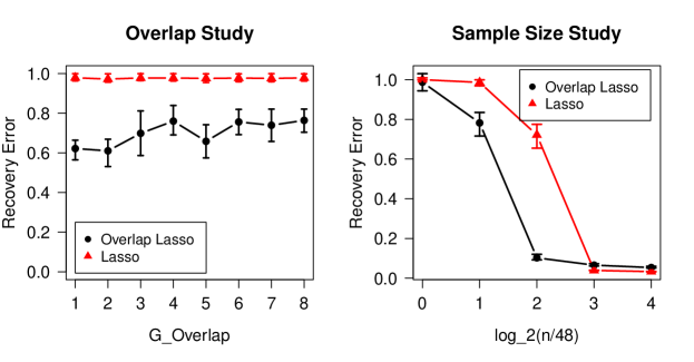
Figure 1: Results of the simulation study. We compare the overlapping grouped lasso to the ordinary lasso. Left: study on the degree of overlap of the groups. Right: study on sample size.

7 Discussion and Conclusions

In the previous two sections, we have given results on the performance of the overlapping grouped lasso in both the finite sample and asymptotic setting. One of the basic steps in practical applications of this procedure is the choice of the collection of groups $\mathcal{G}$. In both cases, we showed that an overly complex choice of $\mathcal{G}$ degrades the theoretical guarantees on the performance of the estimator. In the case where the dimension of the problem is fixed, increasing the number of groups leads to less tight upper bounds on both prediction and estimation in the finite sample case. In the asymptotic setting, nested groups lead to inconsistent selection of the true sparsity pattern. Nonetheless, when $\mathcal{G}$ is suitably chosen, we still see that the procedure retains the theoretical benefits of the grouped lasso demonstrated in previous literature.

In summary, we find that the overlapping grouped lasso is a useful extension of the grouped lasso that must be used with caution. The flexibility allowed by overlapping groups is valuable in many applications, and can encode a wide variety of structures as collections of groups. We have shown that allowing for overlap does not remove many of the theoretical properties and benefits proven for the lasso and grouped lasso. However, the procedure must be used with caution. While the flexible nature of the procedure suggests that the analyst may encode many structures simultaneously, this approach is not supported by the results in this paper.

Appendix A Proofs

A.1 Finite Sample Result

A.1.1 Auxillary Lemmas

Lemma 2.

Let $\chi^{2}_{D}$ be a chi-squared random variable with $D$ degrees of freedom. Then:

$$\mathbb{P}(\chi^{2}_{D}>D+x)\leq\exp\left(-\frac{1}{8}\min\left\{x,\frac{x^{2}}{D}\right\}\right).$$ (45)

Proof.

See Lemma A.1 from Lounici et al. (2009). ∎

Lemma 3.

Let $\alpha,\beta\in\mathbb{R}^{p}$, then, $\forall\mathcal{G}$:

$$\alpha^{T}\beta\leq\mathcal{G}_{\mbox{overlap}}^{1/2}\left(\max_{g}||\alpha_{g}||_{2}\right)||\beta||_{2,1,\mathcal{G}}.$$ (46)

Proof.

Let $\{v^{\beta*}_{g}\}$ denote any decomposition of $\alpha$ minimizing the norm $||\beta||_{2,1,\mathcal{G}}$. Then, beginning with Holder’s inequality the following chain gives the desired result:

$$\alpha^{T}\beta \leq||\alpha||_{\infty}||\beta||_{2}$$ (47)

$$\leq\left|\left|\sum_{g}\alpha_{g}\right|\right|_{\infty}\left|\left|\sum_{g}v^{\beta*}_{g}\right|\right|_{2}$$ (48)

$$\leq\mathcal{G}_{\mbox{overlap}}^{1/2}\left(\max_{g}||\alpha_{g}||_{2}\right)\sum_{g}||v^{\beta*}_{g}||_{2}$$ (49)

$$=\mathcal{G}_{\mbox{overlap}}^{1/2}\left(\max_{g}||\alpha_{g}||_{2}\right)||\beta||_{2,1,\mathcal{G}}.$$ (50)

∎

Lemma 4.

Consider the model in Equation 1. Suppose $|\mathcal{G}|=M\geq 2$, and $n\geq 1$. Assume that the entries of $\epsilon$ are i.i.d. Gaussian with mean 0 and variance $\sigma^{2}$. Let X be normalized so that the the diagonal entries of $\textbf{X}^{T}\textbf{X}/n$ are all equal to 1. Let $\{v_{g}^{\widehat{\beta}-\beta}\}$ denote a decomposition of $\widehat{\beta}-\widehat{\beta}$ minimizing the $||\cdot||_{2,1,\mathcal{G}}$ norm. Let $J=J(\beta^{0})=\{g:v_{g}^{0}\neq 0\}$ be the set of groups that are nonzero in the norm minimizing decomposition of $\beta$. Let:

$$\lambda=\frac{2\sigma\sqrt{\max_{g}|g|}}{\sqrt{n}}\left(1+\frac{A\log M}{\sqrt{\max_{g}|g|}}\right)^{1/2}$$ (51)

Here, $A>8$. Define $q=\min\left(A\sqrt{\min_{g}|g|}/8,8\log M\right)$. Then, with probability at least $1-M^{1-q}$, for any solution $\widehat{\beta}$ to Equation 14, for all $\beta\in\mathbb{R}^{p}$, the following inequality holds:

$$\frac{1}{n}||\textbf{X}(\widehat{\beta}-\beta^{0})||^{2}+\lambda||\widehat{\beta}-\beta||_{2,1,\mathcal{G}} \leq\frac{1}{n}||\textbf{X}({\beta}-\beta^{0})||^{2}+4\lambda\sum_{g\in J}||v_{g}^{\widehat{\beta}-\beta}||.$$ (52)

Proof.

We follow the proof strategy of Lounici et al. (2009). For all $\beta\in\mathbb{R}^{p}$, we have:

$$\frac{1}{n}||X\widehat{\beta}-y||^{2}+2\lambda||\widehat{\beta}||_{2,1,\mathcal{G}}\leq\frac{1}{n}||X{\beta}-y||^{2}+2\lambda||\beta||_{2,1,\mathcal{G}}$$ (53)

Let $y=X\beta^{0}+\epsilon$ to obtain:

$$\frac{1}{n}||X(\widehat{\beta}-\beta^{0})||^{2}\leq\frac{1}{n}||X({\beta}-\beta^{0})||^{2}+\frac{2}{n}\epsilon^{T}X(\widehat{\beta}-\beta)+2\lambda\left(||\beta||_{2,1,\mathcal{G}}-||\widehat{\beta}||_{2,1,\mathcal{G}}\right)$$ (54)

We now examine the second term on the right hand side:

$$\frac{2}{n}\epsilon^{T}X(\widehat{\beta}-\beta) \leq\frac{2\mathcal{G}_{\mbox{overlap}}^{1/2}}{n}\left(\max_{g}||\epsilon^{T}X_{g}||\right)||\widehat{\beta}-\beta||_{2,1,\mathcal{G}}$$ (55)

$$=\frac{2\mathcal{G}_{\mbox{overlap}}^{1/2}}{n}\left(\max_{g}\sqrt{\sum_{j\in g}\left(\sum_{i=1}^{n}X_{ij}\epsilon_{i}\right)^{2}}\right)||\widehat{\beta}-\beta||_{2,1,\mathcal{G}}.$$ (56)

Here, we apply our version of Hölder’s inequality (Lemma 3). We now consider the event:

$$\mathcal{A}=\left\{\frac{1}{n}\left(\max_{g}\sqrt{\sum_{j\in g}\left(\sum_{i=1}^{n}X_{ij}\epsilon_{i}\right)^{2}}\right)\leq\frac{\lambda}{2\mathcal{G}_{\mbox{overlap}}^{1/2}}\right\}.$$ (57)

Note that random variables $V_{g(j)}=\frac{1}{\sigma\sqrt{n}}\sum_{i=1}^{n}X_{ij}\epsilon_{i}$, where $g(j)$ denotes the $jth$ element of $g\in\mathcal{G}$, are standard Gaussian random variables. Within a group, they have a multivariate normal distribution with covariance matrix $\textbf{X}_{g}^{T}\textbf{X}_{g}/(\sigma^{2}n)$, where $\textbf{X}_{g}$ denotes the sub matrix of X consisting of the columns indexed by the group $\textbf{X}_{g}$. It then follows that, provided $\textbf{X}_{g}$ admits a Cholesky decomposition, that $(\textbf{X}_{g}^{T}\textbf{X}_{g})^{-1/2}\textbf{X}_{g}\boldsymbol{\epsilon}/\sigma^{2}n$ is a vector of i.i.d. standard normal random variables. Thus, letting $\rho_{g}$ denote the maximal absolute eigenvalue of $(\textbf{X}_{g}^{T}\textbf{X}_{g})^{-1/2}$, we have $||\textbf{X}_{g}\boldsymbol{\epsilon}/\sigma^{2}n||\leq\rho_{g}||(\textbf{X}_{g}^{T}\textbf{X}_{g})^{-1/2}\textbf{X}_{g}\boldsymbol{\epsilon}/\sigma^{2}n||$ by properties of the operator norm of $(\textbf{X}_{g}^{T}\textbf{X}_{g})^{1/2}$. Now, for any $g\in\mathcal{G}$ define:

$$\gamma_{g}=\frac{2\sigma\sqrt{|g|\mathcal{G}_{\mbox{overlap}}}}{\sqrt{n}}\left(1+\frac{A\log M}{\sqrt{|g|}}\right)^{1/2}.$$ (58)

Note, $\forall g\in\mathcal{G};\ \gamma_{g}\leq\lambda$. Now:

$$\mathbb{P}\left(\sum_{j\in g}\left(\sum_{i=1}^{n}X_{ij}\epsilon_{i}\right)^{2}\geq\frac{\lambda^{2}n^{2}}{4\mathcal{G}_{\mbox{overlap}}}\right) \leq\mathbb{P}\left(\rho_{g}^{2}\chi^{2}_{|g|}\geq\frac{\lambda^{2}n}{4\sigma^{2}\mathcal{G}_{\mbox{overlap}}}\right)$$ (59)

$$\leq\mathbb{P}\left(\chi^{2}_{|g|}\geq\frac{\gamma_{g}^{2}n}{4\sigma^{2}\rho_{g}^{2}\mathcal{G}_{\mbox{overlap}}}\right)$$ (60)

$$=\mathbb{P}\left(\chi^{2}_{|g|}\geq\rho_{g}^{-2}(|g|+A\sqrt{|g|}\log M)\right)$$ (61)

$$\leq\exp\left(-\frac{\rho_{g}^{-2}A\log M}{8}\min\left\{\sqrt{|g|},A\log M\right\}\right)$$ (62)

$$\leq\exp\left(-\frac{\min_{g}[\rho_{g}^{-2}]A\log M}{8}\min\left\{\left(\min_{g}\sqrt{|g|}\right),A\log M\right\}\right)$$ (63)

In the above, we used Lemma 2 for the probability bound on $\chi^{2}$ variables. We now apply the union bound to obtain:

$$\mathbb{P}(\mathcal{A}^{c}) \leq M\exp\left(-\frac{\min_{g}[\rho_{g}^{-2}]A\log M}{8}\min\left\{\left(\min_{g}\sqrt{|g|}\right),A\log M\right\}\right)$$ (64)

$$\leq M^{1-q}$$ (65)

Now, on the event $\mathcal{A}$, we can obtain, from Equation 54:

$$\frac{1}{n}||X(\widehat{\beta}-\beta^{0})||^{2} +\lambda||\widehat{\beta}-\beta||_{2,1,\mathcal{G}}\leq$$ (66)

$$\frac{1}{n}||X({\beta}-\beta^{0})||^{2} +2\lambda\left(||\widehat{\beta}-\beta||_{2,1,\mathcal{G}}+||\beta||_{2,1,\mathcal{G}}-||\widehat{\beta}||_{2,1,\mathcal{G}}\right)$$ (67)

$$\leq\frac{1}{n}||X({\beta}-\beta^{0})||^{2}+4\lambda\sum_{g\in J}||v_{g}^{\widehat{\beta}-\beta}||$$ (68)

Where $\{v_{g}^{\widehat{\beta}-\beta}\}$ denotes a decomposition of $\widehat{\beta}-\widehat{\beta}$ minimizing the $||\cdot||_{2,1,\mathcal{G}}$ norm. Note that the last line follows from the fact that $||\cdot||_{2,1,\mathcal{G}}$ obeys the triangle inequality. This gives us the desired result in Equation 52. ∎

A.1.2 Proof of Theorem 1

Again, we follow the proof strategy of Lounici et al. (2009). Fix a decomposition of $\beta^{0}$: $\{v_{g}^{0}\}$. Let $J=J(\beta^{0})=\{g:v_{g}^{0}\neq 0\}$. Let the event $\mathcal{A}$ in Lemma 4 hold and let $\beta=\beta^{0}$ in the inequality 52:

$$\lambda||\widehat{\beta}-\beta^{0}||_{2,1,\mathcal{G}} \leq 4\lambda\sum_{g\in J}||v^{\widehat{\beta}-\beta^{0}}||,$$ (69)

$$\implies\sum_{g\in J^{c}}||v^{\widehat{\beta}-\beta^{0}}|| \leq 3\sum_{g\in J}||v^{\widehat{\beta}-\beta^{0}}||.$$ (70)

Thus, we can apply Assumption 1 with $\Delta=(\widehat{\beta}-\beta^{0}),\mathcal{V}(\Delta)=\{v^{\widehat{\beta}-\beta^{0}}\}$ to obtain:

$$\sum_{g\in J}\left|\left|v^{\widehat{\beta}-\beta^{0}}\right|\right|\leq\frac{||X(\widehat{\beta}-\beta^{0})||}{\kappa\sqrt{n}}$$ (71)

Again, when the event $\mathcal{A}$ in Lemma 4 hold and for $\beta=\beta^{0}$ in the inequality 52:

$$\frac{1}{n}||\textbf{X}(\widehat{\beta}-\beta^{0})|| \leq 4\lambda\sum_{g\in J}||v^{\widehat{\beta}-\beta^{0}}||$$ (72)

$$\leq\frac{4\lambda}{\kappa\sqrt{n}}||X(\widehat{\beta}-\beta^{0})||$$ (73)

$$\implies\frac{1}{n^{2}}||\textbf{X}(\widehat{\beta}-\beta^{0})||^{2} \leq\frac{16\lambda^{2}}{\kappa^{2}n}$$ (74)

$$\implies\frac{1}{n}||\textbf{X}(\widehat{\beta}-\beta^{0})||^{2} \leq\frac{64\sigma^{2}}{\kappa^{2}n}\left(\max_{g}|g|+A\log M\right)$$ (75)

This corresponds to the result in Equation 22. Equation 23 follows from an analogous chain as the above, beginning with the inequality 69.

A.2 Asymptotic Setting

Before we prove the main result, we give the following lemma.

Lemma 5.

Let Assumption 4 hold. For $g\in G_{Ho}$ $n^{\gamma/2}(||v_{g}^{OLS}||)^{\gamma}$ is $O_{p}(1)$ for $\gamma>0$.

Proof.

By Assumption 4, we may denote $\{v_{g}^{0}\}=\mathcal{V}(\beta^{0})$ as the unique decomposition minimizing the norm $||\beta^{0}||_{2,1,\mathcal{G}}$. To make the dependence on $n$ explicit, we denote $\beta^{OLS}_{n}$ as the ordinary least squares estimate for $\beta^{0}$ using $n$ data points. We know $\beta^{OLS}_{n}\to\beta^{o}$ in probability, as $n\to\infty$. By Assumption 4, there exists an $N$ such that, with high probability, $\beta^{OLS}_{n}$ has a unique decomposition for all $n\geq N$. We denote this unique decomposition as: $\{v_{g}^{OLS,n}\}=\mathcal{V}(\beta^{OLS}_{n})$, minimizing $||\beta^{OLS}_{n}||_{2,1,\mathcal{G}}$.

We next write $\beta^{OLS}_{n}=\beta^{0}+\delta_{n}$, and then define the decomposition $v_{g}^{\delta_{n}}=v_{g}^{0}-v_{g}^{OLS_{n}}$. Recall that for $g\in G_{H_{o}}$, we have $||v_{g}^{0}||=0$ and furthermore $||\beta^{OLS}_{n}||_{2,1,\mathcal{G}}\to||\beta^{0}||_{2,1,\mathcal{G}}$ in probability. Thus, considering the terms in $||\beta^{OLS}_{n}||_{2,1,\mathcal{G}}$ corresponding to those $g\in G_{H_{o}}$ we conclude $||v_{g}^{\delta_{n}}||\to 0$ in probability as $n\to\infty$ for $g\in G_{H_{o}}$.

Finally, for $g\in G_{H_{o}}$: $\sqrt{n}(||v_{g}^{OLS}||)=\sqrt{n}(||v_{g}^{OLS}||-||v_{g}^{0}||)=\sqrt{n}(||v_{g}^{\delta_{n}}||-0)\in O_{p}(1)$. The result then follows for $\gamma>0$ by the continuous mapping theorem. ∎

A.2.1 Proof of Theorem 2

We follow the general proof strategy of Theorem 3.2 from Nardi and Rinaldo (2008), which is adapted from similar results on the lasso from Fu and Knight (2000) and Zou (2006). First, define $\beta_{n}=\beta^{0}+\frac{u}{\sqrt{n}}$. Let $\{v_{g}^{0}\}=\mathcal{V}(\beta^{0});\{v_{g}^{n}\}=\mathcal{V}(\beta^{n})$ be decompositions of $\beta^{0}$ minimizing $||\beta^{0}||_{2,1,\mathcal{G}}$, and $||\beta_{n}||_{2,1,\mathcal{G}}$, respectively. Therefore, the following is a decomposition of $u$: $\forall\ g\in\mathcal{G}$, $v_{g}^{u}=\sqrt{n}(v_{g}^{n}-v_{g}^{0})$.

To begin, we write the objective from Equation 15 (multiplied by $\frac{n}{2}$) as:

$$Q_{n}(u)=\frac{1}{2}\left|\left|\frac{1}{\sqrt{n}}Xu+\epsilon\right|\right|^{2}+\sum_{g}n\lambda\lambda_{n}\left|\left|v^{0}_{g}+\frac{1}{\sqrt{n}}v_{g}^{u}\right|\right|$$

Let:

$$D_{n}(u) =Q_{n}(u)-Q_{n}(0)$$

$$=\left(\frac{1}{2n}u^{T}X^{T}Xu-\frac{1}{\sqrt{n}}u^{T}X\epsilon\right)$$

$$\ +\sqrt{n}\lambda\sum_{g}\lambda_{g}\sqrt{n}\left(\left|\left|v^{0}_{g}+\frac{1}{\sqrt{n}}v^{u}_{g}\right|\right|-||v_{g}^{0}||\right)$$

$$=I_{1,n}+\sum_{g}I_{2,n,g}$$

We now proceed to examine the terms in the second summation. The behavior of these terms depends on the group $g$:

• For $g\in G_{H}$, we have $\lambda_{n}\to 1/||v_{g}^{o}||_{2}^{\gamma}$ in probability, by the uniqueness of the decomposition $\{v_{g}^{0}\}$ along with Assumption 4. Also:

  $$\sqrt{n}\left(\left|\left|v^{0}_{g}+\frac{1}{\sqrt{n}}v^{u}_{g}\right|\right|-||v_{g}^{0}||\right)\to\frac{(v^{u}_{g})^{T}v^{0}_{g}}{||v_{g}^{0}||}.$$

  Since $\sqrt{n}\lambda=o(1)$, then the term $I_{2,n,g}\to 0$.

• For $g\in G_{Hc}$, $n^{\gamma/2}||v^{OLS}_{g}||^{\gamma}=O_{p}(1)$ and:

  $$\sqrt{n}\left(\left|\left|v^{0}_{g}+\frac{1}{\sqrt{n}}v^{u}_{g}\right|\right|-||v_{g}^{0}||\right)=||v^{u}_{g}||.$$

  Since, $n^{(\gamma+1)/2}\lambda\to\infty$, then $I_{2,n,g}\to\infty$.

• For $g\in G_{Ho}$, and $n^{\gamma/2}||v^{OLS}_{g}||^{\gamma}_{2}$ is $O_{p}(1)$ by Lemma 5. As before,

  $$\sqrt{n}\left(\left|\left|v^{0}_{g}+\frac{1}{\sqrt{n}}v^{u}_{g}\right|\right|-||v_{g}^{0}||\right)=||v^{u}_{g}||.$$

  So $I_{2,n,g}\to\infty$.

Now, $I_{1,n}\to\frac{1}{2}u^{T}\mathcal{M}u-u^{T}W$, where $W\sim N_{p}(0,\sigma^{2}\mathcal{M})$. Since $p$ is fixed and finite, then it follows that $D_{n}(u)\to D(u)$, where:

$$D(u)=\left\{\begin{array}[]{lr}\frac{1}{2}u^{T}\mathcal{M}u-u^{T}W&\mbox{if }\forall g\notin G_{H}:v^{u}_{g}=0\\ \infty&\mbox{else}\end{array}\right.$$

Now, $u=(\mathcal{M}_{H}^{-1}W,0)^{T}$ minimizes $D(u)$ and so by the argmax theorem from (van der Vaart and Wellner, 1998, Corollary 3.2.3), the result follows.

References

- Bach (2008a) {barticle}[author] \bauthor\bsnmBach, \bfnmFrancis\binitsF. (\byear2008a). \btitleConsistency of the Group Lasso and Multiple Kernel Learning. \bjournalJournal of Machine Learning Research \bvolume9 \bpages1179–1225. \endbibitem
- Bach (2008b) {binproceedings}[author] \bauthor\bsnmBach, \bfnmFrancis\binitsF. (\byear2008b). \btitleExploring Large Feature Spaces with Hierarchical Multiple Kernel Learning. In \bbooktitleAdvances in Neural Information Processing Systems. \bseriesNIPS ’08. \endbibitem
- Bach (2010a) {btechreport}[author] \bauthor\bsnmBach, \bfnmFrancis\binitsF. (\byear2010a). \btitleShaping Level Sets with Submodular Functions \btypeTechnical Report No. \bnumberarXiv:1012.1501v1. \endbibitem
- Bach (2010b) {binproceedings}[author] \bauthor\bsnmBach, \bfnmFrancis\binitsF. (\byear2010b). \btitleStructured Sparsity-Inducing Norms through Submodular Functions. In \bbooktitleAdvances in Neural Information Processing Systems. \bseriesNIPS ’10. \endbibitem
- Bickel, Ritov and Tsybakov (2009) {barticle}[author] \bauthor\bsnmBickel, \bfnmJ.\binitsJ., \bauthor\bsnmRitov, \bfnmYa acov\binitsY. and \bauthor\bsnmTsybakov, \bfnmAlexandre B.\binitsA. B. (\byear2009). \btitleSimultaneous analysis of Lasso and Dantzig selector. \bjournalAnnals of Statistics \bvolume37 \bpages1705–1732. \endbibitem
- Chesneau and Hebiri (2008) {barticle}[author] \bauthor\bsnmChesneau, \bfnmChristophe\binitsC. and \bauthor\bsnmHebiri, \bfnmMohamed\binitsM. (\byear2008). \btitleSome theoretical results on the Grouped Variables Lasso. \bjournalMathematical Methods of Statistics \bvolume17 \bpages317–326. \endbibitem
- Fu and Knight (2000) {barticle}[author] \bauthor\bsnmFu, \bfnmWenjiang\binitsW. and \bauthor\bsnmKnight, \bfnmKeith\binitsK. (\byear2000). \btitleAsymptotics for lasso-type estimators. \bjournalThe Annals of Statistics \bvolume28 \bpages1356–1378. \endbibitem
- Huang, Zhang and Metaxas (2009) {binproceedings}[author] \bauthor\bsnmHuang, \bfnmJunzhou\binitsJ., \bauthor\bsnmZhang, \bfnmTong\binitsT. and \bauthor\bsnmMetaxas, \bfnmDimitris\binitsD. (\byear2009). \btitleLearning with structured sparsity. In \bbooktitleProceedings of the 26th Annual International Conference on Machine Learning. \bseriesICML ’09 \bpages417–424. \bpublisherACM, \baddressNew York, NY, USA. \endbibitem
- Huang and Zhang (2010) {barticle}[author] \bauthor\bsnmHuang, \bfnmJunzhou\binitsJ. and \bauthor\bsnmZhang, \bfnmTong\binitsT. (\byear2010). \btitleThe Benefit of Group Sparsity. \bjournalAnnals of Statistics \bvolume38 \bpages1978–2004. \endbibitem
- Jacob, Obozinski and Vert (2009) {binproceedings}[author] \bauthor\bsnmJacob, \bfnmLaurent\binitsL., \bauthor\bsnmObozinski, \bfnmGuillaume\binitsG. and \bauthor\bsnmVert, \bfnmJean-Philippe\binitsJ.-P. (\byear2009). \btitleGroup lasso with overlap and graph lasso. In \bbooktitleProceedings of the 26th Annual International Conference on Machine Learning. \bseriesICML ’09 \bpages433–440. \bpublisherACM, \baddressNew York, NY, USA. \endbibitem
- Jenatton, Audibert and Bach (2009) {btechreport}[author] \bauthor\bsnmJenatton, \bfnmRodolphe\binitsR., \bauthor\bsnmAudibert, \bfnmJean-Yves\binitsJ.-Y. and \bauthor\bsnmBach, \bfnmFrancis\binitsF. (\byear2009). \btitleStructured Variable Selection with Sparsity-Inducing Norms \btypeTechnical Report No. \bnumberarXiv:0904.3523v3. \endbibitem
- Jenatton, Obozinski and Bach (2010) {binproceedings}[author] \bauthor\bsnmJenatton, \bfnmRodolphe\binitsR., \bauthor\bsnmObozinski, \bfnmGuillaume\binitsG. and \bauthor\bsnmBach, \bfnmFrancis\binitsF. (\byear2010). \btitleStructured Sparse Principal Component Analysis. In \bbooktitleProceedings of the International Conference on Artificial Intelligence and Statistics. \bseriesAISTATS ’10. \endbibitem
- Kim and Xing (2010) {binproceedings}[author] \bauthor\bsnmKim, \bfnmSeyoung\binitsS. and \bauthor\bsnmXing, \bfnmEric\binitsE. (\byear2010). \btitleTree-Guided Group Lasso for Multi-Task Regression with Structured Sparsity. In \bbooktitleProceedings of the 27th International Conference on Machine Learningy. \bseriesICML ’10. \endbibitem
- Lounici et al. (2009) {binproceedings}[author] \bauthor\bsnmLounici, \bfnmKarim\binitsK., \bauthor\bsnmTsybakov, \bfnmAlexandre B.\binitsA. B., \bauthor\bsnmPontil, \bfnmMassimiliano\binitsM. and \bauthor\bsnmGeer, \bfnmSara A. Van De\binitsS. A. V. D. (\byear2009). \btitleTaking Advantage of Sparsity in Multi-Task Learning. In \bbooktitleCOLT 2009. \endbibitem
- Nardi and Rinaldo (2008) {barticle}[author] \bauthor\bsnmNardi, \bfnmYuval\binitsY. and \bauthor\bsnmRinaldo, \bfnmAlessandro\binitsA. (\byear2008). \btitleOn the asymptotic properties of the group lasso estimator for linear models. \bjournalElectronic Journal of Statistics \bvolume2 \bpages605–633. \endbibitem
- Peng et al. (2010) {barticle}[author] \bauthor\bsnmPeng, \bfnmJie\binitsJ., \bauthor\bsnmZhu, \bfnmJi\binitsJ., \bauthor\bsnmBergamaschi, \bfnmAnna\binitsA., \bauthor\bsnmHan, \bfnmWonshik\binitsW., \bauthor\bsnmNoh, \bfnmDong-Young\binitsD.-Y., \bauthor\bsnmPollack, \bfnmJonathan R.\binitsJ. R. and \bauthor\bsnmWang, \bfnmPei\binitsP. (\byear2010). \btitleRegularized multivariate regression for identifying master predictors with application to integrative genomics study of breast cancer. \bjournalAnnals Of Applied Statistics \bvolume4 \bpages53–77. \endbibitem
- Percival et al. (2011) {barticle}[author] \bauthor\bsnmPercival, \bfnmDaniel\binitsD., \bauthor\bsnmRoeder, \bfnmKathryn\binitsK., \bauthor\bsnmRosenfeld, \bfnmRoni\binitsR. and \bauthor\bsnmWasserman, \bfnmLarry\binitsL. (\byear2011). \btitleStructured, Sparse Regression With Application to HIV Drug Resistance. \bjournalAnnals Of Applied Statistics. \bnoteTo appear. \endbibitem
- Tibshirani (1996) {barticle}[author] \bauthor\bsnmTibshirani, \bfnmRobert\binitsR. (\byear1996). \btitleRegression Shrinkage and Selection Via the Lasso. \bjournalJournal of the Royal Statistical Society, Series B \bvolume58 \bpages267–288. \endbibitem
- van der Vaart and Wellner (1998) {bbook}[author] \bauthor\bparticlevan der \bsnmVaart, \bfnmAad W.\binitsA. W. and \bauthor\bsnmWellner, \bfnmJon A.\binitsJ. A. (\byear1998). \btitleWeak Convergence and Empirical Processes: With Applications to Statistics. \bpublisherSpringer. \endbibitem
- Yuan et al. (2006) {barticle}[author] \bauthor\bsnmYuan, \bfnmMing\binitsM., \bauthor\bsnmYuan, \bfnmMing\binitsM., \bauthor\bsnmLin, \bfnmYi\binitsY. and \bauthor\bsnmLin, \bfnmYi\binitsY. (\byear2006). \btitleModel selection and estimation in regression with grouped variables. \bjournalJournal of the Royal Statistical Society, Series B \bvolume68 \bpages49–67. \endbibitem
- Zhao et al. (2007) {barticle}[author] \bauthor\bsnmZhao, \bfnmPeng\binitsP., \bauthor\bsnmRocha, \bfnmGuilherme\binitsG., \bauthor, and \bauthor\bsnmYu, \bfnmBin\binitsB. (\byear2007). \btitleThe composite absolute penalties family for grouped and hierarchical variable selection. \bjournalAnnals Of Statistics \bvolume37 \bpages3468–3497. \endbibitem
- Zou (2006) {barticle}[author] \bauthor\bsnmZou, \bfnmH\binitsH. (\byear2006). \btitleThe Adaptive Lasso and Its Oracle Properties. \bjournalJournal of the American Statistical Association \bvolume101 \bpages1418-1429. \endbibitem