A Multiband Study of the Galaxy Populations of the First Four
Sunyaev–Zeldovich Effect selected Galaxy Clusters

Abstract

We present first results of an examination of the optical properties of the galaxy populations in SZE selected galaxy clusters. Using clusters selected by the South Pole Telescope survey and deep multiband optical data from the Blanco Cosmology Survey, we measure the radial profile, the luminosity function, the blue fraction and the halo occupation number of the galaxy populations of these four clusters with redshifts ranging from 0.3 to 1. Our goal is to understand whether there are differences among the galaxy populations of these SZE selected clusters and previously studied clusters selected in the optical and the X-ray. The radial distributions of galaxies in the four systems are consistent with NFW profiles with a galaxy concentration of 3 to 6. We show that the characteristic luminosities in $griz$ bands are consistent with passively evolving populations emerging from a single burst at redshift $z=3$. The faint end power law slope of the luminosity function is found to be on average $\alpha\approx-1.2$ in $griz$. Halo occupation numbers (to $m^{*}+2$) for these systems appear to be consistent with those based on X-ray selected clusters. The blue fraction estimated to $0.36L^{*}$, for the three lower redshift systems, suggests an increase with redshift, although with the current sample the uncertainties are still large. Overall, this pilot study of the first four clusters provides no evidence that the galaxy populations in these systems differ significantly from those in previously studied cluster populations selected in the X-ray or the optical.

1. Introduction

Galaxy clusters can be readily discovered or selected using optical or IR emission from their member galaxies, X-ray emission from the hot intracluster medium and now even by the impact of this intracluster medium on the cosmic microwave background temperature toward these systems. First, from optical observations, Abell (1958) identified, catalogued and characterized clusters of galaxies using classification criteria like $compactness$, $distance$, and $richness$. Later, new optical surveys added other optical properties to the clusters. Luminosity function, radial profile, blue fraction, dwarf-to-giant ratio, among others, became tools for understanding different physical processes in the galaxy cluster environment.

With the advent of space based astronomy new properties of clusters of galaxies were discovered. Strong X-ray emission made the galaxy clusters some of the most luminous objects in the universe, and their properties like X-ray luminosity, temperature, and mass have been compiled in several X-ray selected cluster surveys (see, Giacconi et al., 1972; Voges et al., 1999, 2000; Böhringer et al., 2004, for example).

In the infra-red regime, the properties of clusters have been studied mainly relying on the X-ray or optical cluster identification (see, de Propris et al., 1999; Lin et al., 2003, 2004; Toft et al., 2004; De Propris et al., 2007; Muzzin et al., 2007a, b; Roncarelli et al., 2010, among others). From IR selected clusters, some of the first studies analyzed the cluster populations based on individual clusters (Stanford et al., 1997, 2005). Later, systematic searches of clusters in the infrared became feasible with the operation of space telescopes and with ground based telescopes with advanced IR detectors. Surveys such as FLAMEX (Elston et al., 2006), UKIDSS (van Breukelen et al., 2006), FLS (Muzzin et al., 2008) and the IRAC Shallow Survey (Eisenhardt et al., 2008) have delivered cluster catalogs, at high redshift, allowing initial systematic characterization of the galaxy populations on those systems.

In the millimeter regime, the use of the Sunyaev-Zel’dovich Effect (SZE, Sunyaev & Zel’dovich, 1972) as a selection method for cluster of galaxies has recently produced the first results (Staniszewski et al., 2009; Vanderlinde et al., 2010). The use of the SZE effect for cluster detection has several advantages. A catalog of SZE selected clusters is approximately mass limited, nearly redshift independent and the observable signature is closely related to the cluster mass (Birkinshaw, 1999; Carlstrom et al., 2002), making it less prone to be biased in the selection. In particular, an SZE selected cluster sample provides an opportunity to systematically study the galaxy populations and its redshift evolution in clusters of the same mass range over a wide range of redshift.

In this paper we use tools developed for optical studies to analyze the galaxy populations of the first four SZE selected clusters published by the South Pole Telescope (SPT) collaboration (Staniszewski et al., 2009). As well as being among the first SZ selected systems, these clusters are among the most well studied. This sample has been imaged deeply in the optical Blanco Cosmology Survey, studied in the X-ray (Andersson et al., 2010), targeted spectroscopically for redshifts (High et al., 2010), and the BCS data have been used to estimate weak lensing masses (McInnes et al., 2009). Also these four systems span a broad range in redshift and mass, much like the larger samples that have been published so far (Vanderlinde et al., 2010; Williamson et al., 2011). In this pilot study, we study the luminosity function, the radial profile, the Halo Occupation number and the blue fraction, in an effort to answer a basic question: Are the galaxy populations from these first SZE selected clusters any different than the populations in clusters selected by other means?

The paper is organized as follows: §2 describes the observations and data reduction. In section §3, properties of the clusters, such as redshift and mass, are described. In §4 we study the galaxy populations in the clusters, presenting the main results. Conclusion of this study are presented at section §5. Magnitudes are quoted in AB system.

We assume a flat, $\Lambda$CDM cosmology with $H_{0}$ = 100$h$ km s^-1 M$pc^{-1}$, $h$ = 0.702, and matter density $\Omega_{m}$ = 0.272, according to WMAP7 + BAO + $H_{0}$ data (Komatsu et al., 2010).

2. Observations and Data Reduction

2.1. Blanco Cosmology Survey

The Blanco Cosmology Survey (BCS) project was awarded 60 nights from the NOAO (National Optical Astronomy Observatory) survey program starting in semester 2005B. Data were gathered in 2005–2008 using the Blanco 4-meter telescope located at Cerro Tololo Inter-American Observatory in Chile. The telescope is equipped with a wide field camera called the Mosaic2 imager, which consists of an array of eight $2K\times 4K$ CCDs. The pixel scale of Mosaic2 imager is $0.27$ arc-second per pixel, leading to a field of view of about $0.36$ square degree. The observations were carried out to obtain a deep, four band photometric survey ($g$, $r$, $i$ and $z$) of two $50$ deg² patches of the southern sky centered at 23h00m,-55^∘12” and 05h30m,-55^∘47”. These regions were chosen to enable observations by three mm-wavelength survey experiments (the SPT, the Atacama Pathfinder Experiment (APEX) and the Atacama Cosmology Telescope (ACT) experiments). On photometric nights we also observed several standard star fields that contain stars with known magnitudes. This approach allows the calibration of our data to the standard magnitude system. In addition, we obtained deep imaging of several fields overlapping published spectroscopic surveys to enable calibration of photo-z’s using samples of many thousands of spectroscopic redshifts. The data volume we collected for the BCS observation was about $20$ to $30$ Gigabytes/night.

The first three seasons (2005 to 2007) of the BCS imaging data were processed in 2008 and 2009 using version 3 of the data management system developed for the upcoming Dark Energy Survey (DES). Details of the DES data management system can be found in Ngeow et al. (2006) and Mohr et al. (2008). A brief description is presented in this paper. Data parallel processing was carried out primarily on NCSA’s TeraGrid IA-64 Linux cluster. The pipeline processing middleware developed within the DES data management system provides the infrastructure for the automated and robust execution of our parallel pipeline processing on the TeraGrid cluster.

To remove the instrumental signatures, the raw BCS images were processed using the following corrections: crosstalk correction, overscan correction, bias subtraction, flat fielding, fringe and illumination correction. Bad columns and pixels, saturated pixels and bright star halos, and bleed trails are masked automatically. Wide field imagers have field distortions that generally deviate significantly from a simple tangent plane, and there are typically telescope pointing errors as well. The AstrOmatic code SCAMP (Bertin, 2006) was used to refine the astrometric solution by matching the detected stars in BCS images to the USNO-B catalog. We adopted the $PV$ distortion model that maps detector coordinates to sky coordinate using a third order polynomial expansion of distortions, across each CCD, relative to a tangent plane. The DES data management system is using an experimental version of the AstrOmatic tool SExtractor (Bertin & Arnouts, 1996). This experimental version includes model fitting photometry and improved modes of star-galaxy classification to detect and catalog astronomical objects in the images. We harvested a wide range of photometric and astrometric measurements (and their uncertainties) for each object during this cataloging.

For the photometric nights that include observation of the standard star fields, we determined the band dependent (atmospheric) extinction coefficients ($k$) together with CCD and band dependent photometric zeropoints ($a$) and instrumental color terms ($b$). Specifically, the equation we constructed for each star in the standard star fields is $m_{inst}-m_{std}=\sum_{i}w_{i}\times[a_{i}+b_{i}(\Delta C)]+kX$, where $w_{i}=1$ if the standard star is on CCD $i$; $w_{i}=0$ otherwise. In this equation, $m_{inst}$ and $m_{std}$ are the instrumental and the true magnitudes for the standard stars, respectively, $\Delta C$ is the color offset of the standard stars from a reference color, and $X$ is the airmass. The standard star fields include the SDSS Stripe 82 fields and the Southern Standard Stars Network fields. The resulting photometric solutions were then used to calibrate the magnitudes for other astronomical objects observed on the same night.

The nightly reduced and astrometric refined images were remapped and coadded to a pre-defined grid of tiles (which is a rectangular tangent plane projection, with $\sim 36$ arc-minute on a side (hereafter the BCS tiles) in the sky using another AstrOmatic tool, SWarp (Bertin et al., 2002). During this coaddition we carry out a PSF homogenization across each tile and within each band to match the PSF to median delivered seeing in that part of the sky. The zeropoints for the flux scales for these input remap images are determined using different sources of photometric information, including direct photometric zeropoints which are derived from the photometric solution on photometric nights, relative photometric zeropoints determined using all pairs of images that overlap on the sky and the color behavior of the stellar locus (High et al., 2009). We determine the zeropoints for all images by doing a least squares solution using the constraints described above. During co-addition, we use a weighted mean combine option in SWARP. The coadded images are built in each band for a given coadd tile, then a $\chi^{2}$ image (Szalay et al., 1999) is created for detection and cataloging to ensure each object will have measurements in the $griz$ bands extracted from the same portion of the object.

2.2. Completeness

For this work we estimate the completeness of the BCS tiles from the comparison of their $griz$ source count histograms and those extracted from the deeper Canada-France-Hawaii-Telescope Legacy Survey survey (CFHTLS, Brimioulle et al., 2008, private communication). Specifically, we used count histograms from the D-1 1 sqr. degree patch at high galactic latitude (l= $172.0^{\circ}$; b = $-58.0^{\circ}$) from the CFHTLS Deep Field, whose magnitude limit is beyond r=27 and the seeing is better than 1.0” and 0.9” for $g$ and $riz$, respectively . Dividing both count histograms (see Fig. 1) we can estimate the level of completeness in the different tiles in each band. We can use this completeness estimate for each field to account for the missing objects as we approach the full depth of the photometry. Table 1 contains the magnitude limits in each band corresponding to 50% and 90% completeness for the tiles used in our analysis.

Figure 1.— We estimate the completeness of our BCS coadds by comparing objects counts from them with counts from deeper CFHT data. The resulting completeness curve is fitted by an error function, which later is used to correct for the missing galaxies and to define 90% and 50% completeness limits for analysis. Here is an example for the SPT-CL J0516-5430 field.

Table 1Completeness limits for each tile for each filter for 90%/50% completeness

ID	R.A.	decl.	g	r	i	z
	[deg]	[deg]	500 sec	600 sec	1350 sec	705 sec
SPT-CL J0516-5430	79.15569	-54.50062	23.18/24.24	22.73/23.87	22.20/23.47	21.87/23.19
SPT-CL J0509-5342	77.33908	-53.70351	23.72/24.78	23.29/24.51	23.10/24.23	22.45/23.78
SPT-CL J0528-5300	82.02212	-52.99818	23.70/24.62	23.42/24.32	22.93/23.94	22.23/23.37
SPT-CL J0546-5345	86.65700	-53.75861	23.34/24.31	22.87/23.90	22.48/23.64	21.97/23.08

3. Basic Properties of these SPT Clusters

The basic properties of these SPT selected clusters, including the characteristics of the optical counterparts are presented in Staniszewski et al. (2009) and are further discussed in follow on papers (Menanteau et al., 2009; McInnes et al., 2009; High et al., 2010; Andersson et al., 2010). Several spectroscopic redshifts are now available as well as Chandra X-ray observations, providing dramatically improved mass information which enables the kind of galaxy population study we undertake here. Despite being a small sample, these four clusters are among the most well studied SZ selected systems and their mass and redshift distributions range are similar to the whole SPT published cluster sample (see Fig. 2). In particular, these masses and redshifts are used to estimate the projected cluster virial radius in which the optical properties are measured. These properties are presented below.

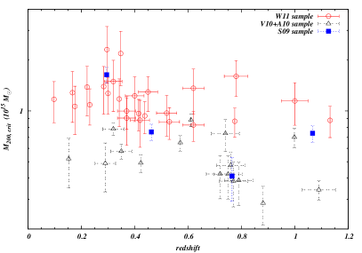
Figure 2.— Masses and redshifts of the SPT cluster sample published to date. Open circles are from Williamson et al. (2011), open triangles are from Andersson et al. (2010) and Vanderlinde et al. (2010), and filled squares from Staniszewski et al. (2009), the sample here studied. The $M_{200,crit}$ mass estimations come from X–ray observations where that is possible, or from the SPT detection significance. In the latter case, masses have been converted from their native estimation $M_{200,mean}$ to $M_{200,crit}$ assuming a concentration parameter of $c=5$ for the halo mass (see table 2) under assumed cosmology. It can be seen that our sample spans on the redshift and mass space for the latest SPT sample.

3.1. Redshifts

The spectroscopic redshifts of the four cluster are now available (Table 2). SPT-CL J0516-5430, a known cluster identified in the Abell supplementary southern catalog (AS0520, Abell et al., 1989) and in the REFLEX survey (RXC J0516.6−5430, Böhringer et al., 2004), had a redshift of 0.294 (Guzzo et al., 1999) and 0.2952 (Böhringer et al., 2004), values obtained using 8 galaxy spectra from the ESO Key Programme.

For the other three clusters, spectroscopic data has recently been acquired. Using LDSS-3 on Magellan Clay telescope, High et al. (2010) reported redshifts of 0.7648 for SPT-CL 0528-5300 and 0.4626 for SPT-CL 0509-5342. For SPT-CL J0546-5345, Brodwin et al. (2010) used IMACS on Baade Magellan telescope to measure a redshift of 1.0665.

3.2. Cluster masses

As mentioned in §3, the optical analyses performed in this work require an estimate of the projected cluster virial radius. For this purpose, along with spectroscopic redshifts, X-ray masses estimations are used. We adopt mass estimates defined with respect to the critical density.

As it has been previously mentioned, SPT-CL 0516-5430 is a previously known cluster, and its mass has also been estimated. With the name of RXC J0516.6-5430 in the REFLEX survey, Zhang et al. (2006) used XMM-Newton to find a $M_{500}$ of (6.4 $\pm$ 2.1) 10${}^{14}\ M_{\odot}$. Also, recent X-ray observations of the four clusters have been performed, and the mass estimation of SPT-CL 0517-5430 has been refined.

Using Chandra and XMM-Newton, Andersson et al. (2010) reported X-ray measurements of 15 of the 21 SZE selected clusters presented in Vanderlinde et al. (2010). The observations of those clusters, which include the original first four clusters, have been designed to deliver around 1500 photons within $0.5r_{500}$, in order to enable measurement of the ICM mass and ICM temperature, allowing a mass estimation through a $M_{500}-Y_{X}$ scaling relation (Vikhlinin et al., 2009) with approximately 15% accuracy.

From X-ray $M_{500,Y_{X}}$ and spectroscopic redshifts Andersson et al. (2010) estimated the physical $r_{500,Y_{X}}$, both defined with respect to the critical density. Here, those $r_{500,Y_{X}}$/$M_{500,Y_{X}}$ are transformed to $r_{200,Y_{X}}$/$M_{200,Y_{X}}$ using the Navarro, Frenk, & White (Navarro et al., 1997, hereafter ’NFW’ profile) radial mass profile with concentration of 5 for the dark matter halo, which implies $r_{200,Y_{X}}=1.51\times r_{500,Y_{X}}$ / $M_{200,Y_{X}}=1.38\times M_{500,Y_{X}}$ conversion. The angular projection is calculated using the spectroscopic redshifts. $M_{200,Y_{X}}$ as well as $r_{200,Y_{X}}$ are listed in Table 2.

Table 2X-ray masses, spectroscopic redshifts and cluster parameters.

ID	$M_{200,Y_{X}}^{a}$	$z$	$r_{200,Y_{X}}^{b}$	$r_{200,Y_{X}}$	$\xi^{c}$	$c_{red\ gal}^{d}$	$c_{all\ gal}^{e}$
	[$10^{14}M_{\odot}$]		[Mpc]	[arcmin]	S/N
SPT-CL J0516-5430	$16.38\pm 1.72$	0.2952f	2.21	8.34	9.42	$4.65^{+0.81}_{-0.73}$	$2.79^{+0.63}_{-0.52}$
SPT-CL J0509-5342	$7.51\pm 0.83$	0.4626g	1.61	4.54	6.61	$3.18^{+3.50}_{-1.39}$	$1.94^{+7.44}_{-1.36}$
SPT-CL J0528-5300	$4.11\pm 1.19$	0.7648g	1.17	2.61	5.45	$5.93^{+5.78}_{-2.58}$	$3.23^{+1.37}_{-0.55}$
SPT-CL J0546-5345	$7.37\pm 0.85$	1.0665h	1.27	2.57	7.69	$4.02^{+1.98}_{-1.37}$	$4.04^{+1.92}_{-1.31}$

4. Cluster Galaxy Populations

The galaxy populations in clusters have been studied using several techniques and selection processes. Clusters of galaxies have been selected mainly from optical images (Abell, 1958; Abell et al., 1989; Koester et al., 2007, for example) and through their X-ray emission (Ebeling et al., 1996; Vikhlinin et al., 1998; Böhringer et al., 2004, among others). A selection of clusters based on their Sunyaev-Zeldovich signature promises a less biased selection method, as it is likely to be less affected by projections or false clusters like optical surveys (Lucey, 1983; Sutherland, 1988; Collins et al., 1995; Cohn et al., 2007), and its mass selection function is nearly redshift independent, making the cluster sample more homogeneous than X-ray surveys in redshift space. Also, the SPT survey will be able to find the most massive clusters of galaxies in the universe (Carlstrom et al., 2002, 2009). Once completed, the size, redshift extent and the degree of completeness of the SZE selected cluster sample will be ideal for statistical analysis of astrophysical properties in high mass clusters. Here we focus on the first four SPT selected clusters, which are all high mass systems extending over a broad redshift range.

4.1. Radial distribution of galaxies

The radial distribution of galaxies in clusters can be used to further our understanding of the cluster environment physics. For example, from N-body and gas dynamical simulations, which include radiative cooling, star formation, SN feedback, UV heating, etc., Nagai & Kravtsov (2005) produced radial distributions consistent with observations of X-ray selected cluster samples from Carlberg et al. (1997) and Lin et al. (2004). Saro et al. (2006), using hydrodynamical simulations, also showed an agreement between the radial distribution of the simulated galaxies and X–ray and optically selected clusters from Popesso et al. (2007a).

For the following analysis we define the cluster center to be the position of the observed brightest cluster galaxy member (BCG; coordinates are listed in Table 1), which agree with its X-ray center (Andersson et al., 2010). In order to compare different studies we estimate the concentration parameter from the NFW surface density profile. We obtain the NFW surface density by integrating the three-dimensional number density profile $n(x)=n_{0}x^{-1}(1+x)^{-2}$ along the line-of-sight (see Bartelmann, 1996) where $x=c_{g}r/r_{200}$, $n_{0}$ is the normalization and $c_{g}$ is the concentration parameter. On stacked cluster data it is customary to fit both parameters, $n_{0}$ and $c_{g}$. In our case the NFW fit is done over single cluster data to a common magnitude limit, and this leads to considerable uncertainties in the parameters of the NFW profile. In order to minimize this problem, we introduce the observed number of galaxies in the equation. Integrating the NFW surface density over the projected area we can derive $n_{0}=n_{0}(n_{obs},c_{g})$ allowing us to fit the NFW density profile as a single parameter function. Also, after a statistical background correction, a background fitting is performed along with the NFW fit. Such background fit is limited within the Poisson uncertainty of the observed background.

Figure 3.— Radial profiles for the red galaxy population to $0.36L^{*}$ (same as blue fraction), binned to obtain similar signal to noise. These profiles are centered on the BCG and extend to 3$r_{200}$ to allow the background and the cluster profile to be fit simultaneously. All radial profiles are consistent with NFW profiles with concentrations $c\sim 4$.

The radial surface density profiles are constructed using both the red+blue and the red galaxy population defined from the color-magnitude diagram of the red sequence (see sec. 4.4). The galaxy population is also selected performing a cut in brightness, selecting galaxies which are fainter than the BCG and brighter than a common limit of $0.36L^{*}$. The error bars are computed using small number statistics (Gehrels, 1986). The background is statistically subtracted and a second correction is applied fitting it to a radius of $3r_{200}$. Finally the data is presented using radial bins of constant signal-to-noise of 3.5 (see Fig. 3).

Some corrections are applied to these profiles. In the area calculation for each radial bin in Fig. 3, the area covered by saturated stars was excluded in order to avoid an under estimation of the surface density. This is especially important in the case of SPT-CL J0509-5342 where several bright stars close to the BCG are blocking the detection of galaxy cluster members, covering about 50% of the area at a radius of $0.4r_{200}$.

The concentration parameters found are shown in Table 2. With a concentration in the range of $c\approx 3-6$, the clusters agree at $1\sigma$ confidence. We note that the blue+red distribution tends to be less concentrated than the red population alone, which is consistent with previous analyses where a higher concentration is seen in the red population (e.g. Goto et al., 2004). The concentration we find is in agreement with concentrations drawn from X-ray selected clusters of galaxies. For example, Carlberg et al. (1997) found a $c_{g}$ of $3.70^{+3.99}_{-1.38}$ at 95% confidence, using 16 clusters from the CNOC survey with a median redshfit of $\sim 0.3$ for a similar mass range ($2\times M_{\odot}^{14}$-$6.6\times M_{\odot}^{15}$; Carlberg et al. (1996)). Lin et al. (2004), from stacked 2MASS K-band data on 93 nearby X-ray selected clusters, found a value of $c_{g}=2.90^{+0.21}_{-0.22}$ in a wider $3\times M_{\odot}^{13}$-$2\times M_{\odot}^{15}$ range. Both are consistent with our results.

We also found agreement between our concentration parameter and the concentration parameter found for optical selected clusters. Biviano & Poggianti (2009) found, studying 19 intermediate redshift ($0.4\lesssim z\lesssim 0.8$; $0.7\lesssim M_{200}\lesssim 13.6\times 10^{14}M_{\odot}$) EDisCS+MORPHS clusters, a concentration parameter of $c=3.2^{+4.6}_{-2.0}$. Also, Johnston et al. (2007) found, using the SDSS sample, a concentration parameter of $c_{200|14}=4.1\pm 0.2_{stat}\pm 1.2_{sys}$ for a cluster mass of $M=10^{14}h^{-1}M_{\odot}$. In summary, we find no evidence that SZE selected clusters exhibit different galaxy radial distributions than in optical and X-ray selected clusters.

Figure 4.— Here we plot the $m^{*}$ (with 1 $\sigma$ uncertainties) for each band that results from Schechter function fits to the luminosity function with free parameters $m^{*}$, $\phi^{*}$ and $\alpha$ ($\alpha$ fixed where noted). We limit the range of $m^{*}$ to be fainter than the identified BCG for each cluster. The continuous line represents a passive evolution single burst model at $z=3$ from Bruzual & Charlot (2003). It is clear that these SPT selected clusters have galaxy populations consistent with this simple evolution model.

4.2. Luminosity functions

The luminosity function (LF) is an important tool for testing theories of galaxy formation and evolution. For example, ever more complex simulations can be tested against the LF, as an observational constraint, to probe our understanding of the evolution of galaxies in the cluster’s environment (Romeo et al., 2005; Saro et al., 2006). With clusters of similar masses we can study the LF as a function of redshift and with the LF parameters we can calculate the Halo Occupation Number (HON) and test the N-M scaling relation (Lin et al., 2004, 2006).

The LF can be described by the three parameter Schechter function (Schechter, 1976),

$$\phi(m)=0.4\ln(10)\ \Phi^{*}10^{0.4(m^{*}-m)(\alpha+1)}\exp(-10^{0.4(m^{*}-m)})$$

where $\Phi^{*}$ is the normalization, $m^{*}$ is the characteristic magnitude and $\alpha$ accounts for the faint end power law behavior of the function.

The construction of the LF is done assuming that the $observed$ LF in the cluster area is the superposition of the cluster LF and the background/foreground non–cluster LF. To recover the cluster LF we subtract the galaxy source count, rescaled by the area, from the observed LF. Given the wide range in redshift we present the LF in the four $griz$ bands.

The area of the cluster is defined by our estimation of $r_{200}$ (see §3.2 and Table 2), and the area of the background is the tile area (36’$\times$36’) minus the cluster area. The bright end limit of the LF is defined by the cluster’s BCG while the faint end limit is defined by its completeness at 90% or 50%, depending on the redshift, in each band. Below the 100% completeness, the 0.5 mag bins are corrected using the error function fitted to the BCS/CFHT comparison galaxy count histograms described in §2.2 and shown in Fig. 1. Finally, the number of galaxies, background corrected, is divided by cluster volume (in M$pc^{3}$) and the uncertainty is assumed Poissonian in the total number of galaxies (cluster plus background).

Below we extract $m^{*}$ and $\alpha$ from our cluster sample and compare them to previous results drawn from X-ray and optical selected clusters of galaxies.

4.2.1 Evolution of $m^{*}$

Studies of $m^{*}$ evolution in clusters have been done in different wavelengths and with different selection methods. These studies indicate that the stellar populations in many of the cluster galaxies have evolved passively after forming at high redshift (see, e.g., Gladders et al., 1998; De Lucia et al., 2004; Holden et al., 2004; Muzzin et al., 2008, and references therein). There are several indications that $m^{*}$ evolution can be described from a single stellar populations (SSP) synthesis model as optical and X-ray selected clusters. All four of these SPT selected clusters in our study show red sequences (see Fig. 11), and their color evolution is consistent with colors derived from a single stellar population (SSP) synthesis model.

In order to perform a direct comparison of the brightness and evolution of the characteristic magnitude, we let all the LF variables vary, where possible, and compare $m^{*}$ in $griz$ bands derived from the LF fitting to that based on the SSP model. The SSP model we use for the red galaxy population is constructed using a Bruzual & Charlot synthesis model (BC03; Bruzual & Charlot, 2003) for the red galaxy populations, assuming a single burst of star formation at z=3 followed by passive evolution to z=0. We use six different models with six distinct metallicities to match the tilt of the color magnitude relation at low redshift, and we add scatter in the metallicity-luminosity relation to reproduce the intrinsic scatter in the color-magnitude relation. These models are then calibrated, using 51 X-ray clusters that have available SDSS magnitudes drawn from the DR7 database. Details of the model used can be found in Song et al (submitted). As shown in Fig. 4, the SSP model and $m^{*}$ in each band are in good agreement, showing that the SSP model is an appropriate description of both the colors and the magnitudes of the more evolved early type galaxies in this sample of SZE selected clusters. We will use this agreement to carry out a more constrained study of the luminosity function.

4.2.2 Faint end slope

To learn about the $\alpha$ behavior we take advantage of the agreement shown in § 4.2.1 between SSP model and the data. We adopt $m^{*}$ from the model (see Table 3) and fit for $\Phi^{*}$ and $\alpha$ for each cluster individually. The study of the faint end slope $\alpha$ provides us with information about the faint galaxy populations in the cluster with respect to the more evolved bright end, which is dominated by luminous early type galaxies. This relation gives us insight into competing processes in the hierarchical structure formation scenario, including the accretion of faint galaxies by the cluster, causing a steep $\alpha$, and the evolution of galaxies inside the cluster through galaxy merging, dynamical friction, star formation quenching and other processes.

Using the $amoeba$ simplex minimization routine (Press et al., 1992), $\Phi^{*}$ and $\alpha$ are chi-square fitted, and their uncertainties are determined by gridding in parameter space (see the LF in Fig. 5, 6, 7, 8, and their contour confidence regions at Fig. 9).

From the literature, we find that our average $\alpha\approx$ -1.2 is in agreement at the 1$\sigma$ level with previous studies which used samples constructed with different selection methods. For example, from an optical work, De Propris et al. (2003) used 60 clusters at z $<$ 0.11 from 2dFGRS in the $b_{J}$ band finding $\alpha=-1.28\pm 0.03$. Paolillo et al. (2001) found, on a composite LF of 39 Abell clusters, an $\alpha$ of $-1.07^{+0.09}_{-0.07}$, $-1.11^{+0.09}_{-0.07}$ and $-1.09^{+0.12}_{-0.11}$ for Gunn $g$, $r$ and $i$ respectively.

From X-ray selected samples Lin et al. (2004) created a composite K-band LF of 93 clusters, finding that the faint-end slope is well fitted by $-1.1\lesssim\alpha\lesssim-0.84$ in agreement with our findings within the errors. Popesso et al. (2005), using 97 X-ray selected clusters with SDSS photometry, for a redshift $z<$ 0.25, found that a better representation of the data is given by two Schechter functions, characterized by a bright and a faint end slope. Comparing to the bright end of the double Schechter function with local background subtraction (which is the most similar case), the bright end slope, in 1 Mpc $h^{-1}$, has a slope $\alpha$ of $-1.23\pm 0.11$, $-1.05\pm 0.13$, $-1.17\pm 0.13$, and $-1.06\pm 0.12$ in $g$, $r$, $i$, and $z$, respectively, also agreeing with our findings at the 1$\sigma$ level.

From IR selected clusters Muzzin et al. (2008) detected 99 clusters and groups of galaxies and constructed the LF in 3.6$\mu$m, 4.5$\mu$m, 5.8$\mu$m, and 8.0$\mu$m. Although the 3.6$\mu$m band is redward of our $griz$ photometry, the LF constructed seems to be consistent with $\alpha\approx-1$.

The agreement found between the multiband LF parameters calculated for our SZE selected clusters, and previous studies of galaxy cluster LFs indicates that the galaxy populations in these SZE selected clusters are not very different from those in clusters selected by other means.

Figure 5.— Here we plot the luminosity function with best fit Schechter function for each band in SPT-CL J0516-5430. Note that the BCG had been removed. Best fit parameters are shown on the figure, while Table 3 includes best fit and 1$\sigma$ uncertainties. 100% and 90% completeness limits are noted with vertical dotted lines in each panel.

Figure 6.— Same as Figure 5 but for SPT-CL J0509-5342.

Figure 7.— Same as Figure 5 but for SPT-CL J0528-5300 with the 100% and 50% completeness limits noted with vertical dotted lines in each panel.

Figure 8.— Same as Figure 7 for SPT-CL J0546-5345 with only $i$ and $z$ bands.

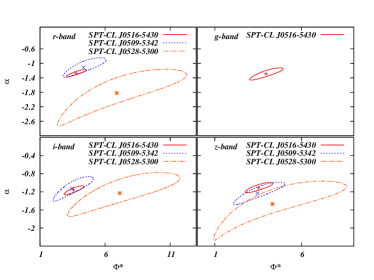
Figure 9.— We plot the 68% confidence region for the LF parameters for each cluster and band combination. Panels are arranged by band with confidence regions for each cluster where a fit for $\alpha$ and $\Phi^{*}$ was possible. The current data suggest steeper than normal faint end parameters $\alpha$ in two of the clusters and there is a tendency for the higher redshift systems to have higher characteristic galaxy densities, as expected in an evolving universe. Values including those at fixed $\alpha$ are given in Table 3.

Table 3HON parameters

ID	$\Phi_{g}^{*}$	$\alpha_{g}$	$m^{*}_{g}$	$HON$	$\chi^{2}$	$\Phi_{r}^{*}$	$\alpha_{r}$	$m^{*}_{r}$	$HON$	$\chi^{2}$
	$[Mpc^{-3}]$			$(m_{g}^{*}+2)$		$[Mpc^{-3}]$			$(m_{r}^{*}+2)$
SPT-CL J0516-5430	$3.95^{+0.98}_{-0.94}$	$-1.29^{+0.16}_{-0.18}$	20.73	$327^{+157}_{-112}$	0.44	$3.78^{+0.81}_{-0.76}$	$-1.27^{+0.10}_{-0.10}$	19.28	$308^{+105}_{-83}$	0.81
SPT-CL J0509-5342	$7.07^{+1.11}_{-1.11}$	-1.1a	22.27	$191^{+30}_{-30}$	0.35	$4.36^{+1.71}_{-1.59}$	$-1.11^{+0.26}_{-0.28}$	20.74	$119^{+95}_{-57}$	0.58
SPT-CL J0528-5300	—	—	24.34	—	—	$6.89^{+5.37}_{-4.54}$	$-1.82^{+0.66}_{-0.91}$	22.52	$149^{+691}_{-122}$	0.16
SPT-CL J0546-5345	—	—	25.92	—	—	—	—	23.85	—	—
ID	$\Phi_{i}^{*}$	$\alpha_{i}$	$m^{*}_{i}$	$HON$	$\chi^{2}$	$\Phi_{z}^{*}$	$\alpha_{z}$	$m^{*}_{z}$	$HON$	$\chi^{2}$
	$[Mpc^{-3}]$			$(m_{i}^{*}+2)$		$[Mpc^{-3}]$			$(m_{z}^{*}+2)$
SPT-CL J0516-5430	$3.59^{+0.78}_{-0.74}$	$-1.17^{+0.10}_{-0.10}$	18.76	$266^{+88}_{-71}$	1.67	$3.52^{+0.82}_{-0.77}$	$-1.11^{+0.11}_{-0.11}$	18.42	$248^{+89}_{-71}$	0.93
SPT-CL J0509-5342	$3.45^{+1.65}_{-1.40}$	$-1.13^{+0.27}_{-0.28}$	19.99	$96^{+87}_{-49}$	0.39	$3.45^{+1.58}_{-1.38}$	$-1.23^{+0.24}_{-0.26}$	19.57	$105^{+92}_{-53}$	0.29
SPT-CL J0528-5300	$7.15^{+4.57}_{-4.02}$	$-1.23^{+0.46}_{-0.52}$	21.42	$84^{+148}_{-58}$	0.64	$4.34^{+4.25}_{-3.46}$	$-1.47^{+0.50}_{-0.82}$	20.78	$65^{+265}_{-56}$	0.51
SPT-CL J0546-5345	$25.43^{+4.03}_{-4.04}$	-1.1a	22.83	$337^{+53}_{-53}$	0.88	$15.2^{+5.57}_{-5.58}$	-1.1a	21.75	$202^{+74}_{-74}$	1.19

4.3. Halo Occupation Number

Based on the Press & Schechter formalism (Press & Schechter, 1974), the halo occupation distribution (HOD) is a powerful analytical tool for understanding the physical processes driving galaxy formation (Seljak, 2000; Berlind et al., 2003). Also the HOD can be used to constrain cosmological parameters (Zheng & Weinberg, 2007).

One of the key ingredients in the HOD formalism is $\langle N\rangle(M)$, the mean number of galaxies per halo or the Halo Occupation Number (HON). In the hierarchical scenario, the HON is expected to increase slower than the mass. While a fraction of the accreted galaxies merged, the galaxy production becomes less efficient as larger haloes are also hotter and less efficient in gas cooling (Cole et al., 2000). Observationally, several studies with cluster samples selected optically and through their X-ray emission have been performed, reinforcing that picture. For example, from samples of optically selected clusters and groups, Marinoni & Hudson (2002) found $N\propto M^{0.83\pm 0.15}$ for systems with $M\gtrsim 10^{13}h_{75}^{-1}M_{\odot}$. Also, Muzzin et al. (2007c) found $N_{500}\propto M_{500}^{0.71\pm 0.11}$ in the $\sim 2\times 10^{14}M_{\odot}-2\times 10^{15}M_{\odot}$ mass range. In the X-ray selection method counterpart, Lin et al. (2004) found, from a sample of 93 nearby clusters and groups, $N\propto M^{0.87\pm 0.04}$. Combining X-ray and optically selected clusters, Popesso et al. (2007a) found $N\propto M_{200}^{0.92\pm 0.03}$. A similar picture was found by Rines et al. (2004), who used nearby X-ray luminous Abell clusters of mass $\sim 3\times 10^{14}h^{-1}M_{\odot}$ and found $N\propto M^{0.74\pm 0.15}$.

Here we test whether the HON of SZE selected clusters exhibits a $N\propto M^{\beta}$, with $\beta<1$, behavior shown by other selection methods.

Due to the small sample presented here, our approach is to construct the HON and compare our results to the N-M scaling relation and evolution constraints obtained by Lin et al. (2004, 2006). That scaling relation is appropriate in this analysis as it covers the mass and redshift range of this SZE sample. The scaling relation was constructed using X-ray selected clusters in the $3\times 10^{13}M_{\odot}$ - $2\times 10^{15}M_{\odot}$ mass range using nearby clusters with 2MASS K-band photometry, and later, Lin et al. (2006), counting galaxies to the depth m*+2, expanded the study to the 0-0.9 redshift range showing that the relation does not strongly evolve.

The Lin et al. (2004) N-M relation is,

$$N_{200}=(36\pm 3)(M_{200}/(10^{14}h^{-1}_{70}M_{\odot}))^{0.87\pm 0.04}$$

To calculate $N_{200}$ we integrate the cluster luminosity function to $L(m_{MODEL}^{*}+2)$ using the parameters of the Schechter luminosity function fit, $\phi_{*}$, L_∗ and $\alpha$ computed in §4.2. The total number of galaxies is

$$N=1+N^{s},\ with\ N^{s}=V\phi_{*}\int^{\infty}_{y_{low}}y^{\alpha}e^{-y}\ dy$$

where the 1 comes from the BCG, which is not part of the LF fitting, V is the cluster volume, and $y_{low}=L_{low}/L_{*}$. We use the derived $M_{200,Y_{X}}$ masses and uncertainties as explained in §3.2 from Andersson et al. (2010) Chandra and XMM observations. The uncertainty in $N_{200}$ is estimated by propagating the 1 $\sigma$ uncertainty in $\phi_{*}$ and $\alpha$ through the integration of the LF to $m^{*}+2$.

The $N_{200}$ with their X-ray mass for the four clusters in the four observed band, along with the HON relation found by Lin et al. (2004), are shown in Fig. 10. Agreement between these SPT clusters and the published results on the X-ray selected sample is good. As with the concentration and the LF faint end, there is no significant evidence that the galaxy properties differ from those already extracted from previous X-ray selected cluster samples.

Figure 10.— We present the halo occupation number (HON(m^∗+2)) within each band for each cluster where the LF is measured in more than three bins. Masses and uncertainties on the horizontal axis come from X-ray analysis of Chandra observations (Andersson et al., 2010). HON uncertainties are derived from the variation of HON due to the 1$\sigma$ uncertainty in the LF ($\alpha$ and $\Phi$*). The dotted lines show the HON derived from a K-band analysis of a large sample of X-ray selected clusters (Lin et al., 2004, 2006). These SPT selected clusters appear to be neither richer nor poorer.

4.4. Blue fractions

Another property of the galaxy populations used to study their evolution in clusters of galaxies is the blue fraction ($f_{b}$). In their seminal work Butcher & Oemler (1984, BO hereafter), using a samples of 33 optically selected clusters of galaxies, estimated $f_{b}$ and showed that it increased with look-back time (termed the Butcher-Oemler effect). Later studies, such as Rakos & Schombert (1995) (0 $<z<$ 1) and Margoniner & de Carvalho (2000) (0.03$\lesssim z\lesssim$0.38), using optically selected clusters, also have found a strong increase in $f_{b}$ with redshift.

With the advent of new optical surveys with hundreds or thousands of clusters the analyses have been strengthened statistically. Using a sample of $\approx$1000 clusters, in a wide redshift range (0$\lesssim z\lesssim$0.9), drawn from the Red-Sequence Cluster Survey (RCS), Loh et al. (2008) found a mild correlation between the red fraction and redshift. Hansen et al. (2009), using thousands of clusters and groups from SDSS, found an evolving $f_{b}$ in the two redshift bins studied (0.1-0.25 and 0.25-0.3), also noticing that $f_{b}$ evolution was weaker for optical masses above $10^{14}h^{-1}M_{\odot}$.

Studies using samples of X-ray selected clusters, have been contradictory. Kodama & Bower (2001) used a sample of seven clusters, in the redshift range of 0.23-0.43, and found a blue fraction trend consistent with BO, while Fairley et al. (2002), using a sample of eight clusters in a 0.23-0.58 redshift range found virtually no trend with redshift. More recently, Urquhart et al. (2010) used CFHT MegaCam $g$ and $r$ photometry on 34 X–ray selected clusters in the redshift range 0.15-0.41 to study $f_{b}$ correlation with other intrinsic cluster properties, found that $f_{b}$ correlated with mass ($T_{X}$) and redshift.

Also there are environmental factors to be considered. Smail et al. (1998) used 10 X-ray selected clusters at similar redshift (0.22 to 0.28) and found a low blue fraction of $\overline{f_{b}}=0.04\pm 0.02$ with a variation of $\Delta f_{b}=0.06$, explained by ’small accretion events’ which contribute blue members to the clusters without much increase of other parameters such as mass or X-ray luminosity. Such events could be a source of scatter in the galaxy populations of clusters selected by any selection method. To analyze $f_{b}$ correlation with other cluster parameters De Propris et al. (2004) used a sample of clusters from 2dF Galaxy Redshift Survey (2dFGRS) at redshift $<$ 0.11, finding a large variation ($f_{b}\sim$ 0.1-0.5 for $M^{*}+1.5$ at $r_{200}$) from cluster to cluster.

The apparent contradiction between X-ray and optically selected samples and the sensitivity to environmental effects, raises questions about how much of the observed $f_{b}$ is due to a selection method, how much it is due to the intrinsic scatter, and if these two effects can conspire to produce an apparent trend where no trend exists.

What is needed is a sample of galaxy clusters which possess two main characteristics: (1) the selection of clusters is made in a way that is independent of the quantity whose evolution is being studied to avoid possible bias (Newberry et al., 1988; Andreon & Ettori, 1999), and (2) the sample must contain the same class of clusters (i.e. same mass range) at different redshift to help in separating mass trends from redshift evolution (Andreon & Ettori, 1999). A sample of SZE selected clusters of galaxies fulfills these requirements. The selection of the SZE clusters is closely related to mass, and that mass selection is approximately independent of redshift, allowing a comparison of the same type of clusters at different epochs.

Figure 11.— Color magnitude diagram for galaxies around each cluster. The blue population is defined to be more than 0.22 mags bluer than the red sequence. Selection in magnitude uses the BCG on the bright end and $m^{*}+\delta$ on the faint end, where this limit corresponds to the 90% completeness limit for SPT-CL J0528-5300 ($0.36L^{*}_{MODEL}$). The visually identified red sequence cluster galaxies are shown using circles.

Historically $f_{b}$ has been measured in different ways. Initially the average color of the E/S0 galaxies, within a radius of R₃₀ from the cluster center that is the radius that contains 30% of all galaxies that belong to the cluster, and a concentration index, were use to define $f_{b}$ (see Butcher & Oemler, 1984; Rakos & Schombert, 1995; Margoniner & de Carvalho, 2000; Fairley et al., 2002). Another approach is using the red sequence from the color-magnitude diagram of the clusters and $r_{200}$ (Popesso et al., 2007b; Barkhouse et al., 2007) or a combination of both methods, that is using the color-magnitude diagram but R₃₀ (Kodama & Bower, 2001; Fairley et al., 2002).

Here we follow the approach of using the red sequence to define the red and blue populations, and $r_{200}$ to define the radial extent. This ensures we are using the same portion of the cluster virial region, independent of redshift, and that we are exploring populations with colors defined with respect to a passively evolving SSP model.

The galaxies used for the $f_{b}$ measurement are inside the $r_{200}$ cluster radius and are fainter than the BCG and brighter than $0.36L^{*}_{MODEL}$. They are classified as red if they are located within $\pm$3 times the average dispersion of the Gaussian fit to the color-magnitude relation ($\pm$ 0.22 mag; López-Cruz et al., 2004), and blue if they are more than 0.22 mags bluer than the Red Sequence. We choose a limit of $0.36L^{*}_{MODEL}$ to allow a meaningful comparison among three of our four clusters, as it is the deepest magnitude that we can detect with good completeness for the three of them. For the fourth cluster, SPT-CL J0546-5345, we currently do not have deep enough photometry for this analysis.

The color magnitude diagram used for the clusters depends on the red sequence identification: g-i/i for SPT-CL J0516-5430, r-i/i for SPT-CL J0509-5342, and i-z/z for SPT-CL J0528-5300 and SPT-CL J0546-5345 (see fig.  11). The blue fraction is defined as the statistically background corrected number of blue galaxies $n_{b}$ divided by the total number of statistically background corrected galaxies $n_{t}$. The blue fraction and its gaussian propagated uncertainty are:

$$f_{b}=\frac{n_{b}}{n_{r}+n_{b}};\ \ \sigma_{f_{b}}^{2}=\sum_{i=r,b}\left(\frac{\partial{f}}{\partial{n_{i}}}\right)^{2}\sigma_{n_{i}}^{2}$$ (1)

Where $n_{b}$ and $n_{r}$ are the blue and red statistically background subtracted number of galaxies:

$$n_{i}=N_{i}-\overline{N}_{i}^{(bkg)}$$

The uncertainties are expressed as

$$\sigma_{n_{i}}^{2}=\sigma_{N_{i}}^{2}+\sigma_{\overline{N}_{i}^{(bkg)}}^{2}$$

assuming $\sigma_{N_{i}}$ Poissonian. The last term is calculated directly by measuring the RMS of the Gaussian distribution observed on histograms constructed from the blue and red (or total) number of galaxies background corrected in a circle of radius $r_{200}$ on $n$ random position outside the cluster radius (background($r_{200}$)-$\overline{background}$) in order to account for background variations on the observed 36’$\times$36’ patch of the sky.

A special mention for SPT-CL 0509-5342 is required. In the center of the cluster are three bright stars leaving only a few visible galaxies; we have corrected this effect by accounting for the area masked around these stars. Nevertheless, the statistical background subtraction leads to negative blue galaxy counts in the $\sim 0.6r_{200}$ inner part of the cluster area.

The blue fraction of three of the four clusters, at redshifts 0.295, 0.463 and 0.763, are shown in Fig. 12. The measurements suggest an increase with redshift, as shown for optically selected clusters, although the result could be consistent with a constant blue fraction over the range of redshift that we explored with our limited sample. Future optical follow up of SPT-SZE selected clusters using larger aperture telescopes on the high redshift end will be necessary to understand the Butcher-Oemler effect in this cluster mass range within the SZE selected sample.

Figure 12.— Blue fraction versus redshift using the populations shown in Figure 11. The Butcher & Oemler (1984) relation is shown (dashed line). The blue fraction is calculated using statistical background correction within $r_{200}$ and to a depth of $0.36L^{*}_{MODEL}$ for each system.

5. Conclusions

We present the results of a careful examination of the multiband optical properties of the galaxy populations in the first four SZE selected galaxy clusters. This analysis builds upon the selection by the South Pole Telescope survey, deep multiband optical data from the Blanco Cosmology Survey, Chandra and XMM mass estimates and published spectroscopic redshifts.

The radial distributions of galaxies in the four systems are consistent with NFW profiles with low concentration in the 2.2-3.6 range, although the constraints in our highest redshift clusters are weak due to the imaging depth. One system shows a clear secondary peak, which is evidence of multiple galaxy components. The observed galaxy concentrations in these SPT systems are consistent with X-ray and optical selected cluster samples as well as simulations.

We showed that the characteristic luminosities in bands $griz$ are consistent with passively evolving populations emerging from a single burst at redshift $z=3$. This is observed by direct comparison of the $griz$ $m^{*}$ measurements with the evolution of the red sequence expected from the SSP model.

The slope of the luminosity function, $\alpha$, in all four bands showed an average of $-1.2$ consistent with previous studies and roughly independent of redshift, although in the high redshift systems the constraints are weaker and the $\Phi-\alpha$ contours are much more extended (see Fig. 9) due to the depth of the data.

Halo occupation numbers (to $m^{*}+2$) for these systems appear to be consistent with the relation measured in X-ray selected clusters. As shown previously (Lin et al., 2004), this well behaved and simple galaxy populations is unfortunately not easy to use as a mass indicator with optical data alone, because the HON varies with the adopted virial radius of the cluster.

The blue fractions $f_{b}$ observed in these systems are consistent with those seen in clusters selected using other means. Although the meassured $f_{b}$ suggest a redshift evolution (as optical studies show), it is within the errors also consistent with a constant $f_{b}$. It is clear that definitive conclusions should be drawn with a larger number of clusters for more robust statistics. A larger sample and deeper multiband data on the high redshift end is needed.

The SPT selection provides a powerful means of choosing similar mass systems over a broad range of redshift, making the future larger cluster sample particularly interesting for this study.

In summary, our systematic analysis of the galaxy populations in the first SZE selected galaxy clusters spanning the redshift range $0.3<z<1.1$ provides no clear evidence that the galaxy populations in these SPT selected clusters differ from populations studied in other X-ray and optically selected samples. An extension of our analysis to the full SPT sample will enable a more precise test of the effects of selection. In addition, comparison of the observed properties of the SPT cluster galaxy populations and their evolution to numerical simulations of galaxy formation should allow for clean tests of the range of physical processes that are responsible in determining the formation and evolution of cluster galaxies.

References

- Abell (1958) Abell, G. O. 1958, ApJS, 3, 211
- Abell et al. (1989) Abell, G. O., Corwin, Jr., H. G., & Olowin, R. P. 1989, ApJS, 70, 1
- Andersson et al. (2010) Andersson, K., et al. 2010, ArXiv e-prints, 1006.3068
- Andreon & Ettori (1999) Andreon, S., & Ettori, S. 1999, ApJ, 516, 647
- Barkhouse et al. (2007) Barkhouse, W. A., Yee, H. K. C., & López-Cruz, O. 2007, ApJ, 671, 1471
- Bartelmann (1996) Bartelmann, M. 1996, A&A, 313, 697
- Berlind et al. (2003) Berlind, A. A., et al. 2003, ApJ, 593, 1
- Bertin (2006) Bertin, E. 2006, in Astronomical Society of the Pacific Conference Series, Vol. 351, Astronomical Data Analysis Software and Systems XV, ed. C. Gabriel, C. Arviset, D. Ponz, & S. Enrique, 112–+
- Bertin & Arnouts (1996) Bertin, E., & Arnouts, S. 1996, A&AS, 117, 393
- Bertin et al. (2002) Bertin, E., Mellier, Y., Radovich, M., Missonnier, G., Didelon, P., & Morin, B. 2002, in Astronomical Society of the Pacific Conference Series, Vol. 281, Astronomical Data Analysis Software and Systems XI, ed. D. A. Bohlender, D. Durand, & T. H. Handley, 228–+
- Birkinshaw (1999) Birkinshaw, M. 1999, Physics Reports, 310, 97
- Biviano & Poggianti (2009) Biviano, A., & Poggianti, B. M. 2009, ArXiv e-prints, 0912.0365
- Böhringer et al. (2004) Böhringer, H., et al. 2004, A&A, 425, 367
- Brimioulle et al. (2008) Brimioulle, F., Lerchster, M., Seitz, S., Bender, R., & Snigula, J. 2008, ArXiv e-prints, 0811.3211
- Brodwin et al. (2010) Brodwin, M., et al. 2010, ApJ, 721, 90
- Bruzual & Charlot (2003) Bruzual, G., & Charlot, S. 2003, MNRAS, 344, 1000
- Butcher & Oemler (1984) Butcher, H., & Oemler, Jr., A. 1984, ApJ, 285, 426
- Carlberg et al. (1996) Carlberg, R. G., Yee, H. K. C., Ellingson, E., Abraham, R., Gravel, P., Morris, S., & Pritchet, C. J. 1996, ApJ, 462, 32
- Carlberg et al. (1997) Carlberg, R. G., et al. 1997, ApJ, 485, L13+
- Carlstrom et al. (2009) Carlstrom, J. E., et al. 2009, submitted to PASP, arXiv:0907.4445
- Carlstrom et al. (2002) Carlstrom, J. E., Holder, G. P., & Reese, E. D. 2002, ARA&A, 40, 643
- Cohn et al. (2007) Cohn, J. D., Evrard, A. E., White, M., Croton, D., & Ellingson, E. 2007, MNRAS, 382, 1738
- Cole et al. (2000) Cole, S., Lacey, C. G., Baugh, C. M., & Frenk, C. S. 2000, MNRAS, 319, 168
- Collins et al. (1995) Collins, C. A., Guzzo, L., Nichol, R. C., & Lumsden, S. L. 1995, MNRAS, 274, 1071
- De Lucia et al. (2004) De Lucia, G., et al. 2004, ApJ, 610, L77
- De Propris et al. (2003) De Propris, R., et al. 2003, MNRAS, 342, 725
- De Propris et al. (2004) ——. 2004, MNRAS, 351, 125
- de Propris et al. (1999) de Propris, R., Stanford, S. A., Eisenhardt, P. R., Dickinson, M., & Elston, R. 1999, AJ, 118, 719
- De Propris et al. (2007) De Propris, R., Stanford, S. A., Eisenhardt, P. R., Holden, B. P., & Rosati, P. 2007, AJ, 133, 2209
- Ebeling et al. (1996) Ebeling, H., Voges, W., Bohringer, H., Edge, A. C., Huchra, J. P., & Briel, U. G. 1996, MNRAS, 281, 799
- Eisenhardt et al. (2008) Eisenhardt, P. R. M., et al. 2008, ApJ, 684, 905
- Elston et al. (2006) Elston, R. J., et al. 2006, ApJ, 639, 816
- Fairley et al. (2002) Fairley, B. W., Jones, L. R., Wake, D. A., Collins, C. A., Burke, D. J., Nichol, R. C., & Romer, A. K. 2002, MNRAS, 330, 755
- Gehrels (1986) Gehrels, N. 1986, ApJ, 303, 336
- Giacconi et al. (1972) Giacconi, R., Murray, S., Gursky, H., Kellogg, E., Schreier, E., & Tananbaum, H. 1972, ApJ, 178, 281
- Gladders et al. (1998) Gladders, M. D., Lopez-Cruz, O., Yee, H. K. C., & Kodama, T. 1998, ApJ, 501, 571
- Goto et al. (2004) Goto, T., Yagi, M., Tanaka, M., & Okamura, S. 2004, MNRAS, 348, 515
- Guzzo et al. (1999) Guzzo, L., et al. 1999, The Messenger, 95, 27
- Hansen et al. (2009) Hansen, S. M., Sheldon, E. S., Wechsler, R. H., & Koester, B. P. 2009, ApJ, 699, 1333
- High et al. (2010) High, F. W., et al. 2010, ApJ, 723, 1736
- High et al. (2009) High, F. W., Stubbs, C. W., Rest, A., Stalder, B., & Challis, P. 2009, AJ, 138, 110
- Holden et al. (2004) Holden, B. P., Stanford, S. A., Eisenhardt, P., & Dickinson, M. 2004, AJ, 127, 2484
- Johnston et al. (2007) Johnston, D. E., et al. 2007, ArXiv e-prints, 0709.1159
- Kodama & Bower (2001) Kodama, T., & Bower, R. G. 2001, MNRAS, 321, 18
- Koester et al. (2007) Koester, B. P., et al. 2007, ApJ, 660, 239
- Komatsu et al. (2010) Komatsu, E., et al. 2010, accepted by ApJS, arXiv:1001.4538
- Lin et al. (2006) Lin, Y., Mohr, J. J., Gonzalez, A. H., & Stanford, S. A. 2006, ApJ, 650, L99
- Lin et al. (2003) Lin, Y., Mohr, J. J., & Stanford, S. A. 2003, ApJ, 591, 749
- Lin et al. (2004) ——. 2004, ApJ, 610, 745
- Loh et al. (2008) Loh, Y., Ellingson, E., Yee, H. K. C., Gilbank, D. G., Gladders, M. D., & Barrientos, L. F. 2008, ApJ, 680, 214
- López-Cruz et al. (2004) López-Cruz, O., Barkhouse, W. A., & Yee, H. K. C. 2004, ApJ, 614, 679
- Lucey (1983) Lucey, J. R. 1983, MNRAS, 204, 33
- Margoniner & de Carvalho (2000) Margoniner, V. E., & de Carvalho, R. R. 2000, AJ, 119, 1562
- Marinoni & Hudson (2002) Marinoni, C., & Hudson, M. J. 2002, ApJ, 569, 101
- McInnes et al. (2009) McInnes, R. N., Menanteau, F., Heavens, A. F., Hughes, J. P., Jimenez, R., Massey, R., Simon, P., & Taylor, A. 2009, MNRAS, 399, L84
- Menanteau et al. (2009) Menanteau, F., et al. 2009, ApJ, 698, 1221
- Mohr et al. (2008) Mohr, J. J., et al. 2008, in Society of Photo-Optical Instrumentation Engineers (SPIE) Conference Series, Vol. 7016, Society of Photo-Optical Instrumentation Engineers (SPIE) Conference Series
- Muzzin et al. (2008) Muzzin, A., Wilson, G., Lacy, M., Yee, H. K. C., & Stanford, S. A. 2008, ApJ, 686, 966
- Muzzin et al. (2007a) Muzzin, A., Yee, H. K. C., Hall, P. B., Ellingson, E., & Lin, H. 2007a, ApJ, 659, 1106
- Muzzin et al. (2007b) Muzzin, A., Yee, H. K. C., Hall, P. B., & Lin, H. 2007b, ApJ, 663, 150
- Muzzin et al. (2007c) ——. 2007c, ApJ, 663, 150
- Nagai & Kravtsov (2005) Nagai, D., & Kravtsov, A. V. 2005, ApJ, 618, 557
- Navarro et al. (1997) Navarro, J. F., Frenk, C. S., & White, S. D. M. 1997, ApJ, 490, 493
- Newberry et al. (1988) Newberry, M. V., Kirshner, R. P., & Boroson, T. A. 1988, ApJ, 335, 629
- Ngeow et al. (2006) Ngeow, C., et al. 2006, in Society of Photo-Optical Instrumentation Engineers (SPIE) Conference Series, Vol. 6270, Society of Photo-Optical Instrumentation Engineers (SPIE) Conference Series
- Paolillo et al. (2001) Paolillo, M., Andreon, S., Longo, G., Puddu, E., Gal, R. R., Scaramella, R., Djorgovski, S. G., & de Carvalho, R. 2001, A&A, 367, 59
- Popesso et al. (2007a) Popesso, P., Biviano, A., Böhringer, H., & Romaniello, M. 2007a, A&A, 464, 451
- Popesso et al. (2007b) Popesso, P., Biviano, A., Romaniello, M., & Böhringer, H. 2007b, A&A, 461, 411
- Popesso et al. (2005) Popesso, P., Böhringer, H., Romaniello, M., & Voges, W. 2005, A&A, 433, 415
- Press & Schechter (1974) Press, W., & Schechter, P. 1974, ApJ, 187, 425
- Press et al. (1992) Press, W. H., Teukolsky, S. A., Vetterling, W. T., & Flannery, B. P. 1992, Numerical recipes in C. The art of scientific computing, ed. Press, W. H., Teukolsky, S. A., Vetterling, W. T., & Flannery, B. P. (Cambridge: University Press, —c1992, 2nd ed.)
- Rakos & Schombert (1995) Rakos, K. D., & Schombert, J. M. 1995, ApJ, 439, 47
- Rines et al. (2004) Rines, K., Geller, M. J., Diaferio, A., Kurtz, M. J., & Jarrett, T. H. 2004, AJ, 128, 1078
- Romeo et al. (2005) Romeo, A. D., Portinari, L., & Sommer-Larsen, J. 2005, MNRAS, 361, 983
- Roncarelli et al. (2010) Roncarelli, M., Pointecouteau, E., Giard, M., Montier, L., & Pello, R. 2010, A&A, 512, A20+
- Saro et al. (2006) Saro, A., Borgani, S., Tornatore, L., Dolag, K., Murante, G., Biviano, A., Calura, F., & Charlot, S. 2006, MNRAS, 373, 397
- Schechter (1976) Schechter, P. 1976, ApJ, 203, 297
- Seljak (2000) Seljak, U. 2000, MNRAS, 318, 203
- Smail et al. (1998) Smail, I., Edge, A. C., Ellis, R. S., & Blandford, R. D. 1998, MNRAS, 293, 124
- Stanford et al. (2005) Stanford, S. A., et al. 2005, ApJ, 634, L129
- Stanford et al. (1997) Stanford, S. A., Elston, R., Eisenhardt, P. R., Spinrad, H., Stern, D., & Dey, A. 1997, AJ, 114, 2232
- Staniszewski et al. (2009) Staniszewski, Z., et al. 2009, ApJ, 701, 32
- Sunyaev & Zel’dovich (1972) Sunyaev, R. A., & Zel’dovich, Y. B. 1972, Comments on Astrophysics and Space Physics, 4, 173
- Sutherland (1988) Sutherland, W. 1988, MNRAS, 234, 159
- Szalay et al. (1999) Szalay, A. S., Connolly, A. J., & Szokoly, G. P. 1999, AJ, 117, 68
- Toft et al. (2004) Toft, S., Mainieri, V., Rosati, P., Lidman, C., Demarco, R., Nonino, M., & Stanford, S. A. 2004, A&A, 422, 29
- Urquhart et al. (2010) Urquhart, S. A., Willis, J. P., Hoekstra, H., & Pierre, M. 2010, ArXiv e-prints, 1004.0020
- van Breukelen et al. (2006) van Breukelen, C., et al. 2006, MNRAS, 373, L26
- Vanderlinde et al. (2010) Vanderlinde, K., et al. 2010, submitted to ApJ, arXiv:1003.0003
- Vikhlinin et al. (2009) Vikhlinin, A., et al. 2009, ApJ, 692, 1060
- Vikhlinin et al. (1998) Vikhlinin, A., McNamara, B., Forman, W., Jones, C., Quintana, H., & Hornstrup, A. 1998, ApJ, 502, 558
- Voges et al. (1999) Voges, W., et al. 1999, A&A, 349, 389
- Voges et al. (2000) ——. 2000, VizieR Online Data Catalog, 9029, 0
- Williamson et al. (2011) Williamson, R., et al. 2011, ArXiv e-prints, 1101.1290
- Zhang et al. (2006) Zhang, Y.-Y., Böhringer, H., Finoguenov, A., Ikebe, Y., Matsushita, K., Schuecker, P., Guzzo, L., & Collins, C. A. 2006, A&A, 456, 55
- Zheng & Weinberg (2007) Zheng, Z., & Weinberg, D. H. 2007, ApJ, 659, 1