Two proposals for testing quantum contextuality of continuous-variable states

Abstract

We investigate the violation of non-contextuality by a class of continuous variable states, including variations of entangled coherent states (ECS’s) and a two-mode continuous superposition of coherent states. We generalise the Kochen-Specker (KS) inequality discussed in A. Cabello, Phys. Rev. Lett. 101, 210401 (2008) by using effective bidimensional observables implemented through physical operations acting on continuous variable states, in a way similar to an approach to the falsification of Bell-CHSH inequalities put forward recently. We test for state-independent violation of KS inequalities under variable degrees of state entanglement and mixedness. We then demonstrate theoretically the violation of a KS inequality for any two-mode state by using pseudo-spin observables and a generalized quasi-probability function.

I Introduction

Non-contextuality is commonly intended as a property of mutually compatible observables. Two observables $A$ and $B$ are said to be compatible when the outcome of a measurement of $A$ performed on a system does not depend on any prior or simultaneous measurement of $B$. A set of mutually compatible observables defines a context, so that the above examples defines a situation where the measurement of A does not depend on the context or is non-contextual. Clearly, non-contextuality is a property inherent in the classical world. In a maieutic game played by Alice and Bob, if Alice asks a question, then clearly the answer is not affected by any prior or simultaneous compatible question asked by Bob.

For quantum observables to assume such a property may at first hand seem reasonable. It would be equally reasonable to assume functional consistency (realism), i.e. for the commuting operators $A_{1}$, $A_{2}$ and $A_{3}=f(A_{1},A_{2})$ to assume that the results of their measurements (even if not performed) would satisfy the same relation as the operators, e.g. $a_{1}$, $a_{2}$ and $f(a_{1},a_{2})$. On the other hand, the two assumptions taken together are incompatible with quantum mechanics.

In fact, the Kochen-Specker (KS) theorem Specker1 ; Specker2 ; Specker3 states that no non-contextual hidden variable (NCHV) theory can reproduce quantum mechanics. This is complementary to the well-known Bell theorem bell , which states that no local hidden variable theory can reproduce quantum mechanics and provides an equally viable tool to gaining insight into the open question to where exactly the boundary between the classical and quantum may lie. Kochen and Specker Specker2 originally produced a set of 117 observables, associated with the squares of the components of the angular momentum operator along 117 different directions to demonstrate a contradiction with non-contextuality. Almost twenty five years later, Peres found a much simpler counter-example peres involving only six Pauli spin operators in the four-dimensional space of two spin-${1}/{2}$ particles. Peres’ formulation of the problem, however, is strictly dependent on the form of the state of the two particles. Mermin mermin made a further simplification by extending the example to include three additional operators, thereby illustrating state-independence. The state-independent nature of the KS theorem is a rather distinctive feature: inequalities based on non-contextual hidden variable theories (herein dubbed as KS inequalities) might be violated by any quantum state, regardless of their degree of entanglement.

It should be remarked how the falsification of a KS inequality faces rather challenging hurdles related to the feasibility of tests that, while are capable of maintaining state independence, also guarantee that all the necessary observables are measured in a context-independent way guhene . Cabello cabello has recently addressed these points by providing inequalities that strictly meet the criteria mentioned above. One such inequality is built from the observables used in the proof of the KS theorem for two qubit systems proposed by Peres and Mermin peres ; mermin . In a seminal experiment, Kirchmair et al. Kirchmair have demonstrated the violation of such an inequality using trapped ions, were two energy levels of an ion are selected so as to embody the single-qubit logical states. The KS inequality was thus tested using ten different quantum states, ranging from entangled to separable, from quasi-pure to almost fully mixed states, hence providing compelling evidence of the state-independent character of the inequality being probed.

Any experimentally testable state-independent KS inequality proposed so far deal with states belonging to Hilbert spaces of finite dimension and dichotomic observables. Plastino and Cabello Plastino have extended the notion of quantum contextuality to include harmonic oscillators by deriving a KS inequality involving 18 observables based on position and momentum. Their conclusion is that it may indeed be possible to experimentally reveal state-independent quantum contextuality for any quantum system admitting two continuous position observables and corresponding canonically conjugate momenta. However, the required measurements might be quite demanding to implement in actual experiments using specific physical systems.

Here, at variance with Plastino and Cabello, we tackle the falsification of non-contextuality inequalities in unbounded Hilbert spaces using a different viewpoint. In fact, while we keep the dichotomic structure of the observable entering the KS inequalities to test, we explicitly consider systems living in infinite-dimensional Hilbert spaces. In order to accomplish our goal, we take advantage of the well-known possibility to violate Bell-like inequalities using dichotomic non-Gaussian observables and continuous-variable (CV) systems prepared in quantum correlated Gaussian states Banaszek ; Chen as well as non-Gaussian states embedding a qubit state Jeong ; Paternostro . In particular, two-mode entangled coherent states (ECSs) sanders and binned homodyne detections have been used by Stobińska et al. Stobinska to show the violation of a Bell-Clauser-Horn-Shimony-Holt (Bell-CHSH) inequality up to Tsirelson’s bound (i.e. the maximum degree of violation allowed by quantum mechanics). In this case, the observables needed for the Bell-CHSH inequality are given by effective rotations built form a series of Kerr non-linearities, displacement operations and phase shifters. This approach to ‘mimic’ the standard Bell-CHSH inequality proved to be quite efficient in demonstrating further the nonlocal properties of highly mixed states close to classicality jeong , non-local realism MP ; lee and multipartite non-locality of a class of multi-qubit states GMcK .

On a parallel line, motivated by feasibility in quantum optical systems, dichotomic observables based on on/off photodetection have been extensively employed to demonstrate violation of Bell-CHSH inequalities using realistic, not fully efficient, photodetectors with either qubit-like states or genuinely continuous-variable ones ban02 ; cinv05 ; so05 . In this paper, we take a similar approach to show that a KS inequality can be violated, in a state independent manner, using qubit states encoded into genuinely infinite dimensional systems. We use the same inequality as in Ref. Kirchmair , which is constructed by means of the effective bidimensional observables that have been exploited for Bell-CHSH inequalities mentioned above. While, on one hand, the number of observables necessary for our task is strictly the same as for discrete-variable systems, our proposal may pave the way to a foreseeable experimental implementation faithful to the constraint of context independence. We then further our study to test a KS inequality using a class of states that do not embed an effective qubit state.This makes the formulation of an analogy with the discrete-system case quite problematic. The paradigm for such a situation is embodied by a two-mode squeezed state. We overcome the difficulties by using the ‘pseudo-spin’ formalism introduced in Ref. Chen . Maximum violation of the KS inequality proves interesting for this class of states that, in the limit of infinite squeezing, approximate the original version of the Einstein-Podolski-Rosen (EPR) state and thus strengthen the claim on the nonexistence of a hidden variable theory to describe quantum mechanics. We generalize our approach by proving that it is indeed possible to violate a KS inequality with any bipartite state of two harmonic oscillators, such as two modes of the radiation field. To achieve this we used a generalised $P$ representation to describe any two-mode state Glauber . As we show, the application of pseudo-spin operators to construct the KS inequality warrants state-independence.

The remainder of this paper is organized as follows. In Sec. II we briefly review the KS formalism, introduce the non-contextual inequality that will be tested throughout our work and introduce the class of effective two-qubit operations with which we build up the observables to be used. Sec. III assesses the violation of the KS inequality by a CV class of Werner state, which we build using ECS form of entangled states (we defer to an Appendix the more formal aspects of our study). We show that, regardless of the degree of entanglement and purity that characterize the states, a large enough amplitude of the coherent states involved guarantees for the state-independent maximum violation of a KS inequality. The case of pseudo-spin operators applied to a test-bed state embodied by a two-mode squeezed vacuum is discussed in Sec. IV and then generalized to any two-mode state, towards full state independence, in Sec. V. Finally, in Sec. VI we summarize our results and leave some open questions.

II Kochen-Specker inequality and general formalism

II.1 The KS inequality

We briefly introduce and discuss the KS inequality that has been experimentally tested in Ref. Kirchmair and is assessed in this paper. The inequality is constructed using nine observables, along the lines of the arguments put forward by Peres and Mermin peres ; mermin to prove the incompatibility between quantum mechanics and non-contextuality. Such observables are arranged in a 3$\times$3 array $\hat{\bm{A}}$, known as the Peres-Mermin square, in such a way that the entries $\hat{A}_{ij}~{}(i,j{=}1,2,3)$ in each column and row are mutually compatible and have dichotomic outcomes $\nu{(\hat{A}_{ij})}{=}\pm{1}$. Denote the products of rows and columns as

$$\hat{R}_{k} =\hat{A}_{k1}\hat{A}_{k2}\hat{A}_{k3}$$

$$\hat{C}_{k} =\hat{A}_{1k}\hat{A}_{2k}\hat{A}_{3k}\,,$$

respectively: Assuming non-contextuality implies that

$$\nu(\hat{R}_{k}) =\nu(\hat{A}_{k1})\nu(\hat{A}_{k2})\nu(\hat{A}_{k3})$$

$$\nu(\hat{C}_{k}) =\nu(\hat{A}_{1k})\nu(\hat{A}_{2k})\nu(\hat{A}_{3k})\,.$$

Thus the total product becomes $\Pi_{k=1}^{3}\nu(R_{k})\nu(C_{k})=1$, since any $\nu(\hat{A}_{ij})$ appears twice in the product. However, this is in contrast with the predictions of quantum mechanics, where a Peres-Mermin square can be built out of the dichotomic Pauli operators

$$\hat{\sigma}_{x}=\begin{pmatrix}0&1\\ 1&0\end{pmatrix},~{}~{}\hat{\sigma}_{y}=\begin{pmatrix}0&-i\\ i&0\end{pmatrix},~{}~{}\hat{\sigma}_{z}=\begin{pmatrix}1&0\\ 0&-1\end{pmatrix},~{}~{}$$

associated with two spin-$1/2$ systems as

$$\hat{\bm{A}}=\left[\begin{matrix}\hat{\sigma}_{z}^{(1)}{\otimes}\hat{\openone}^{(2)}&\hat{\openone}^{(1)}{\otimes}\hat{\sigma}_{z}^{(2)}&\hat{\sigma}_{z}^{(1)}{\otimes}\hat{\sigma}_{z}^{(2)}\\ \hat{\openone}^{(1)}{\otimes}\hat{\sigma}_{x}^{(2)}&\hat{\sigma}_{x}^{(1)}{\otimes}\hat{\openone}^{(2)}&\hat{\sigma}_{x}^{(1)}{\otimes}\hat{\sigma}_{x}^{(2)}\\ \hat{\sigma}_{z}^{(1)}{\otimes}\hat{\sigma}_{x}^{(2)}&\hat{\sigma}_{x}^{(1)}{\otimes}\hat{\sigma}_{z}^{(2)}&\hat{\sigma}_{y}^{(1)}{\otimes}\hat{\sigma}_{y}^{(2)}\end{matrix}\right]$$ (1)

In this case, the product of each row and column gives $\openone$, except those of the last column that gives $-\openone$. Hence, in this case we have the additional property of compatibility for $\hat{R}_{k}$ and $\hat{C}_{k}$ (k=1,2,3) and so, assuming non-contextuality, $\Pi_{k=1}^{3}\nu(\hat{R}_{k})\nu(\hat{C}_{k}){=}\nu\left(\Pi_{k=1}^{3}\hat{R}_{k}\hat{C}_{k}\right){=}{-}1$. This witnesses the contradiction between a non-contextual assumption and the predictions of quantum mechanics. Such a conflicting outcome is formalized by the KS-like inequality cabello

$$\langle\hat{\chi}_{{}_{\hbox{\footnotesize\sc ks}}}\rangle=\langle\hat{R}_{1}\rangle+\langle\hat{R}_{2}\rangle+\langle\hat{R}_{3}\rangle+\langle\hat{C}_{1}\rangle+\langle\hat{C}_{2}\rangle-\langle\hat{C}_{3}\rangle\leq 4.$$ (2)

In Ref. cabello it has been proven that this inequality is bounded by 4 for any NCHV theory, while $\langle\hat{\chi}_{{}_{\hbox{\footnotesize\sc ks}}}\rangle=6$ for any state of two spin-$1/2$ particles. Eq. (2) will be used throughout this paper.

II.2 General formalism for CV states and effective bidimentional dichotomic observables

In this Section we introduce the class of CV states of interest and the effective observables necessary for the falsification of the KS inequality discussed above. The class of state that will be used in the first part of our work are built on coherent states $\left|\alpha\right\rangle$ ($\alpha{\in}\mathbb{C}$), which are obtained by applying the displacement operator $\hat{D}(\alpha){=}\exp(\alpha\hat{a}^{\dagger}{-}\alpha^{\ast}\hat{a})$ to the vacuum state $\left|0\right\rangle$ barnett . Here, $\hat{a}$ ($\hat{a}^{\dagger}$) is the annihilation (creation) operator of a bosonic system. Although two coherent states with opposite phases $\left|\alpha\right\rangle$ and $\left|-\alpha\right\rangle$ are strictly non-orthogonal, we have $\left\langle\alpha|-\alpha\right\rangle{=}\exp[-2|\alpha|^{2}]{\rightarrow}0$ in the limit of $\alpha{\gg}{1}$. In such conditions, $\{\left|\alpha\right\rangle,\left|-\alpha\right\rangle\}$ form a basis in a two-dimensional Hilbert space. This reasoning paves the way for extending the KS inequality in Eq. (2) to deal with CV systems represented in the coherent-state qubit basis. As it will be clarified in Sec. III, in our investigation we consider mixed states of two coherent-state qubits having a variable degree of entanglement between them.

The second important point is embodied by the provision of appropriate observables able to mimic the Pauli spin-${1}/{2}$ ones entering $\hat{\bm{A}}$ in Eq. (1). To do this, we take advantage of the results reported in Stobinska ; MP , where effective rotations are introduced in order to run a Bell-CHSH test. Such operations are generally given by the 2$\times$2 transformation matrix acting on the space spanned by the coherent-state qubit $\{\left|\alpha\right\rangle,\left|-\alpha\right\rangle\}$

$$\hat{O}(\theta,\phi)=\left(\begin{array}[]{cc}\sin\frac{\theta}{2}&\text{e}^{i\phi}\cos\frac{\theta}{2}\\ \text{e}^{-i\phi}\cos\frac{\theta}{2}&-\sin\frac{\theta}{2}\\ \end{array}\right).$$ (3)

For proper choices of parameters $\theta\in[0,\pi]$ and $\phi\in[0,2\pi]$, any spin-$1/2$ transformation can be realized. Eq. (3) can be simulated by a sequence of building-block operations given by displacement operations given by $\hat{D}(i\eta/2\alpha)$ (for proper choices of $\eta\in\mathbb{C}$) and the single-mode Kerr-like nonlinearity $\hat{U}_{NL}{=}\exp[-i\pi(\hat{a}^{\dagger}\hat{a})^{2}/2]$ walls . More precisely, a simulation of Eq. (3) is provided by

$$\hat{O}(\theta,\phi)\simeq\hat{D}(-i\phi/4\alpha)\hat{U}_{NL}\hat{D}(i\theta/4\alpha)\hat{U}_{NL}\hat{D}(i\phi/4\alpha),$$ (4)

where the symbol $\simeq$ is used to remind that the approximation improves as $|\alpha|$ grows. The explicit transformations experienced by $\left|\pm\alpha\right\rangle$ are given by MP

$$\left|\alpha\right\rangle\rightarrow\frac{1}{2}\left[\text{e}^{\frac{i\theta}{4}}\left(\left|\alpha+\frac{i\theta}{4\alpha}\right\rangle+i\text{e}^{\frac{i\phi}{2}}\left|-\alpha-\frac{i\phi}{2\alpha}-\frac{i\theta}{4\alpha}\right\rangle\right)\right.$$ (5)

$$\left.+i\text{e}^{-\frac{i\theta}{4}}\left(\text{e}^{\frac{i\phi}{2}}\left|-\alpha-\frac{i\phi}{2\alpha}+\frac{i\theta}{4\alpha}\right\rangle+i\left|\alpha-\frac{i\theta}{4\alpha}\right\rangle\right)\right],$$

$$\left|-\alpha\right\rangle\rightarrow\frac{1}{2}\left[i\text{e}^{\frac{i\theta}{4}}\left(i\left|-\alpha-\frac{i\theta}{4\alpha}\right\rangle+\text{e}^{\frac{-i\phi}{2}}\left|\alpha-\frac{i\phi}{2\alpha}+\frac{i\theta}{4\alpha}\right\rangle\right)\right.$$

$$\left.+\text{e}^{-\frac{i\theta}{4}}\left(i\text{e}^{-\frac{i\phi}{2}}\left|\alpha-\frac{i\phi}{2\alpha}-\frac{i\theta}{4\alpha}\right\rangle+\left|-\alpha+\frac{i\theta}{4\alpha}\right\rangle\right)\right].$$

Eqs. (5) are crucial in the construction of $\langle\hat{\chi}_{{}_{\hbox{\footnotesize\sc ks}}}\rangle$.

(a)                                               (b)                                               (c)      

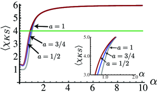
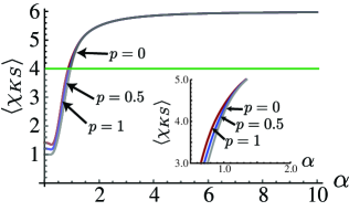
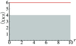
Figure 1: (a) Violation of non-contextuality by a CV Werner state at increasing values of the amplitude $\alpha\in\mathbb{R}$. We plot three KS functions, each corresponding to $p=1$ in Eq. (6). The three curves correspond to $a=1,3/4$ and $1/2$. Maximum violation of the non-contextual KS inequality in Eq. (2) is achieved independently of the degree of entanglement. The inset shows a magnification of the region given by $\alpha\in[0.5,2]$. In panel (b) we have plotted the KS functions corresponding to $a=0.5$, thereby working with maximally entangled coherent states, for $p=1,0.5$ and $0$ in a CV Werner state. Maximum violation of the KS inequality is achieved, regardless of the degree of mixedness within the state. The inset shows a magnification of the region given by $\alpha\in[0.5,2]$. (c) Violation of KS inequality by a two mode-squeezed state plotted against the squeezing parameter $r$. The KS inequality is given by Eq. (2), where the Pauli observables within each $\hat{A}_{ij}$ are replaced by the corresponding pseudo-spin operator in Eq. (12). In all the panels, the shaded region corresponds to the constraints imposed by NCHV theories on the KS function.

III Violation of the KS inequality by a CV Werner state

Here, we discuss the performance of the KS inequality when tested using a CV Werner-like class of states. These are defined as

$$\rho_{w}(a,p)= {p}\left|\text{ECS}(a)\rangle\langle\text{ECS}(a)\right|+$$ (6)

$$\frac{1}{4}(1-p)\Big{[}\left|\alpha,\alpha\rangle\langle\alpha,\alpha\right|{+}\left|\alpha,-\alpha\rangle\langle\alpha,-\alpha\right|$$

$$+\left|-\alpha,\alpha\rangle\langle-\alpha,\alpha\right|{+}\left|-\alpha,-\alpha\rangle\langle-\alpha,-\alpha\right|\Big{]}\,.$$

State $\left|\text{ECS}(a)\right\rangle$ denotes a pure ECS reading

$$\left|\text{ECS}(a)\right\rangle{=}N(\sqrt{a}\left|\alpha,\alpha\right\rangle{+}\sqrt{1{-}a}\left|-\alpha,-\alpha\right\rangle)\,,$$

whose degree of entanglement is parameterised by $a\in[0,1]$ with

$$N{=}[1{+}2\sqrt{(1-a)a}\text{e}^{-4|\alpha|^{2}}]^{-1/2}$$

being a normalization factor. For $a{=}0,1$ the state is fully separable, while at $a{=}{1}/{2}$ and $|\alpha|\gg{1}$ it approximates a maximally entangled two-qubit Bell state. The parameter $p\in[0,1]$ accounts for the degree of mixedness of $\rho_{w}(a,p)$, which is a statistical mixture (a pure ECS state) for $p=0$ ($p=1$). The combined tuning of $a$ and $p$ gives us access to a broad range of states that can be used to test the KS inequality for a state-independent violation.

The KS function $\langle\hat{\chi}_{{}_{\hbox{\footnotesize\sc ks}}}\rangle$ for this Werner-like class of states is built from the correlators $\langle\hat{R}_{i}\rangle$, $\langle\hat{C}_{i}\rangle$ ($i=1,2,3$) as in Eq. (2). Given the general transformation matrix defined by Eq. (3), the Pauli spin-1/2 matrices $\hat{\sigma}_{x}$, $\hat{\sigma}_{y}$ and $\hat{\sigma}_{z}$ are given by $\hat{O}(\theta=0,\phi=0)$, $\hat{O}(\theta=0,\phi=-\pi/2)$ and $\hat{O}(\theta=\pi,\phi=0)$, respectively. The correlator $\langle\hat{\Gamma}_{i}\rangle$ ($\hat{\Gamma}\in\{\hat{R},\hat{C}\}$ and $i\in\{1,2,3\}$) is written as

$$\langle\hat{\Gamma}_{i}\rangle ={(1-p)}\!\sum_{s_{1,2}=\pm}{\left\langle s_{1}\alpha,s_{2}\alpha\right|\hat{\Gamma}_{i}\left|s_{1}\alpha,s_{2}\alpha\right\rangle}/{4}$$ (7)

$$+p\left\langle\text{ECS}(a)\right|\hat{\Gamma}_{i}\left|\text{ECS}(a)\right\rangle$$

where

$$\left\langle\text{ECS}(a)\right|\hat{\Gamma}_{i}\left|\text{ECS}(a)\right\rangle=a\left\langle\alpha,\alpha\right|\hat{\Gamma}_{i}\left|\alpha,\alpha\right\rangle$$ (8)

$$+\sqrt{a(1-a)}(\left\langle\alpha,\alpha\right|\hat{\Gamma}_{i}\left|-\alpha,-\alpha\right\rangle+h.c.)$$

$$+(1-a)\left\langle-\alpha,-\alpha\right|\hat{\Gamma}_{i}\left|-\alpha,-\alpha\right\rangle.$$

Each correlator, $\hat{\Gamma}_{i}$, is given more explicitly in table 1 written in terms of the Pauli operators, described by the general transformation matrix in Eq. (3).

Table 1: Table providing the explicit products of general transformation matrices for each correlator building the KS function $\langle\hat{\chi}_{{}_{\hbox{\footnotesize\sc ks}}}\rangle$.

$\hat{\Gamma}_{i}$	Operator products entering the Peres-Mermin square
$\hat{R}_{1}$	$\left[\hat{O}^{(1)}(\pi,0)\otimes\hat{\openone}^{(2)}\right]\times\left[\hat{\openone}^{(1)}\otimes\hat{O}^{(2)}(\pi,0)\right]\times\left[\hat{O}^{(1)}(\pi,0)\otimes\hat{O}^{(2)}(\pi,0)\right]$
$\hat{R}_{2}$	$\left[\hat{\openone}^{(1)}\otimes\hat{O}^{(2)}(0,0)\right]\times\left[\hat{O}^{(1)}(0,0)\otimes\hat{\openone}^{(2)}\right]\times\left[\hat{O}^{(1)}(0,0)\otimes\hat{O}^{(2)}(0,0)\right]$
$\hat{R}_{3}$	$\left[\hat{O}^{(1)}(\pi,0)\otimes\hat{O}^{(2)}(0,0)\right]\times\left[\hat{O}^{(1)}(0,0)\otimes\hat{O}^{(2)}(\pi,0)\right]\times\left[\hat{O}^{(1)}(0,-\pi/2)\otimes\hat{O}^{(2)}(0,-\pi/2)\right]$
$\hat{C}_{1}$	$\left[\hat{O}^{(1)}(\pi,0)\otimes\hat{\openone}^{(2)}\right]\times\left[\hat{\openone}^{(1)}\otimes\hat{O}^{(2)}(0,0)\right]\times\left[\hat{O}^{(1)}(\pi,0)\otimes\hat{O}^{(2)}(0,0)\right]$
$\hat{C}_{2}$	$\left[\hat{\openone}^{(1)}\otimes\hat{O}^{(2)}(\pi,0)\right]\times\left[\hat{O}^{(1)}(0,0)\otimes\hat{\openone}^{(2)}\right]\times\left[\hat{O}^{(1)}(0,0)\otimes\hat{O}^{(2)}(\pi,0)\right]$
$\hat{C}_{3}$	$\left[\hat{O}^{(1)}(\pi,0)\otimes\hat{O}^{(2)}(\pi,0)\right]\times\left[\hat{O}^{(1)}(0,0)\otimes\hat{O}^{(2)}(0,0)\right]\times\left[\hat{O}^{(1)}(0,-\pi/2)\otimes\hat{O}^{(2)}(0,-\pi/2)\right]$

The decomposition and effective realization of the transformation matrices $\hat{O}(0,0)$, $\hat{O}(0,-\pi/2)$ and $\hat{O}(\pi,0)$ are given in Eq. (4), while the result of their application to $\left|\pm\alpha\right\rangle$ is determined by using Eq. (5). The corresponding explicit form of the correlators as functions of $\alpha$, $p$ and $a$ are too lengthy to be shown here. However, the expressions are analytic and allow us to obtain the full behavior of the KS function $\langle\hat{\chi}_{{}_{\hbox{\footnotesize\sc ks}}}\rangle$ against $\alpha$, for any degree of entanglement and mixedness.

(a)                                    (b)

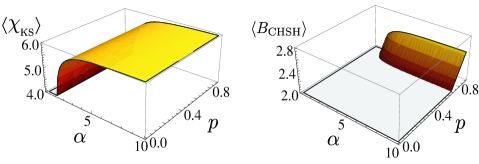
Figure 2: (Color online) (a): Violation of the KS inequality Eq. (2) by a CV Werner state with $a=1/2$. We plot $\langle\chi_{{}_{\hbox{\footnotesize\sc ks}}}\rangle$ against the amplitude $\alpha$ and the purity parameter $p$. As discussed in Fig. 1 (b), the violation of the KS inequality is quasi-insensitive to variations of $p$. (b): Violation of Bell-CHSH inequality by a CV Werner state with $a=1/2$, plotted against $\alpha$ and $p$. As purity grows, $\langle\hat{B}_{\text{CHSH}}\rangle$ violates the local realistic bound of $2$.

In Fig. 1 (a) and (b), we show two significant cases of the quasi-state independence of the KS function $\langle\hat{\chi}_{{}_{\hbox{\footnotesize\sc ks}}}\rangle$ achieved in our model (for simplicity, we have taken $\alpha\in\mathbb{R}$). The analytic expression for each KS function is given, for completeness, in the Appendix. Here, we focus on the general features of such functions. Panel (a) is for $p=1$ and three different values of the entanglement within the state, from full separability to maximum entanglement. On the other hand, panel (b) studies the effects that mixedness has on the behavior of $\langle\hat{\chi}_{{}_{\hbox{\footnotesize\sc ks}}}\rangle$. We set $a=0.5$, so that the CV Werner state is maximally entangled, and tune $p$ from a fully pure state to maximum mixedness. The results are clear: at small amplitudes of the coherent states involved in $\rho_{w}(a,p)$, the KS function is an increasing function that trespasses the bound imposed by NCHV’s in a narrow region around $\alpha{\sim}1$. In these conditions, we observe some minor dependence of the KS function from the various states being used. Those having larger degrees of entanglement and purity become larger than $4$ for slightly smaller values of $\alpha$. The situation changes as the amplitude grows, nullifying the differences highlighted above and delivering a truly state-independent KS function that quickly reaches $6$, the value that is known to be achieved by $\langle\hat{\chi}_{{}_{\hbox{\footnotesize\sc ks}}}\rangle$ in the discrete-variable case and regardless of the state being used. Although Figs. 1 (a) and (b) address only a few significant cases, we have checked that the description provided here is valid for any other choice of $a$ and $p$.

It is also interesting to compare the predictions for non-classicality given by the violation of a KS inequality to those regarding the violation of a local realism Specker3 ; bell . By following the approach described and used in Refs. Stobinska ; jeong ; MP , one can easily build up the Bell-CHSH function $\hat{B}_{{}_{\hbox{\footnotesize\sc chsh}}}$ associated with state $\rho_{w}(a,p)$ in Eq. (6) by means of local rotations realized through the operator $\hat{O}(\theta,\phi)$ and dichotomized homodyne projections onto quadrature eigenstates. In the qubit case, the violation the Bell-CHSH inequality requires rotations performed only on the equatorial plane of the Bloch sphere and this feature is carried over to the case at hand here. We thus have to consider the set of transformations (5) obtained by setting $\phi{=}0$. Moreover, we can restrict the study to projections onto the eigenstates $\left|x\right\rangle$ of the position-like quadrature $(\hat{a}+\hat{a}^{\dagger})/\sqrt{2}$ of a bosonic system barnett . Using the general formula for the projection of a coherent state $\left|\alpha\right\rangle$ (with $\alpha=\alpha_{r}+i\alpha_{i}$) over a position-like quadrature eigenstates $\left|x\right\rangle$

$$\langle{x}|\alpha\rangle=\frac{1}{\sqrt[4]{2\pi}}\text{e}^{i\alpha\alpha_{i}-(x/2-\alpha)^{2}}$$ (9)

one can evaluate $\hat{B}_{{}_{\hbox{\footnotesize\sc chsh}}}$ analytically and then maximize it numerically over the parameters of the local rotations. The results are given in Fig. 2, where a comparison is performed between the Bell-CHSH function and the KS one corresponding to $\rho_{w}(1/2,p)$ (we have taken $a=1/2$ here simply as a significant representative of the general behavior observed for an arbitrary choice of $a$). While panel (a) summarizes the findings reported in Fig. 1 (b), i.e. the quasi-independence of $\langle\hat{\chi}_{{}_{\hbox{\footnotesize\sc ks}}}\rangle$ of the value of $p$ entering the state under scrutiny, panel (b) shows the sensitivity of a Bell-CHSH test to the degree of mixedness of $\rho_{w}(1/2,p)$. This is in line with the idea that KS tests are expected to be generally more powerful than CHSH ones in revealing the quantumness of a physical system.

IV Violation of the KS inequality by a continuous superposition of coherent states

We would like now to extend the class of systems that we use for our goals from the discrete superposition of quasi-orthogonal states that builds up an ECS to a continuous distribution. As the archetypal example of such case, we consider the state produced by superimposing a single-mode squeezed state to a vacuum mode at a 50:50 beam splitter barnett ; knight . The former can be written in the coherent-state basis as the continuous Gaussian-weighted distribution ${\cal N}\int\!d\alpha\,{\cal G}(r,\alpha)\left|\alpha\right\rangle$ with

$${\cal G}(r,\alpha)={\text{e}}^{-\frac{(1-\tanh r)\alpha^{2}}{2\tanh r}},~{}~{}~{}(\alpha\in\mathbb{R})$$ (10)

where $r$ is the squeezing parameter and ${\cal N}{=}1/\sqrt{2\pi\sinh r}$ is the normalization factor knight . It is worth stressing that such a choice of resource state does not limit the validity of the results to come and is merely due to the experimental-friendly nature of the state, which can be routinely produced in many linear-optics labs. Any other choice would be equally valid for our purposes. After the admixture at the beam splitter, we get the two-mode state Paternostro

$$\left|\xi\right\rangle={\cal N}\int\!\!d\alpha\,{\cal G}(r,\alpha)\,|{{\alpha}/{\sqrt{2}},{\alpha}/{\sqrt{2}}}\rangle.$$ (11)

For this class of states any attempt to violate the KS inequality given in Eq. (2) by applying the same set of observables as done for the Werner state, would be meaningless because of the difficulties in identifying, in $\left|\xi\right\rangle$, a bipartite bidimensional system: although the series of displacement operators and Kerr-like nonlinearities introduced above can be used to sufficiently approximate the Pauli matrices entering each $\hat{A}_{ij}$, the possibility of relating the state $\left|\xi\right\rangle$ to that of a ‘two-qubit coherent state’ is undermined by the continuous nature of the distribution in Eq. (11).

However it is not futile to try and falsificate the KS inequality (2) by choosing a different set of observables than those assessed so far. Our reasoning originates from the results by Chen et al. Chen , whereby a generalisation of the Bell-CHSH inequality for two-qubit systems to a two-mode state obtained superimposing a single-mode squeezed vacuum state with a vacuum state at a balanced beam splitter has been shown to be possible. In Ref. Chen , the Bell-CHSH function for the two-mode squeezed vacuum state is built from “pseudo-spin” operators having the form

$$\hat{s}_{x} =\sum_{n=0}^{\infty}\left(\left|2n+1\rangle\langle 2n\right|+\left|2n\rangle\langle 2n+1\right|\right),$$ (12)

$$\hat{s}_{y} =i\sum_{n=0}^{\infty}\left(\left|2n\rangle\langle 2n+1\right|-\left|2n+1\rangle\langle 2n\right|\right),$$

$$\hat{s}_{z} =\sum_{n=0}^{\infty}\left(\left|2n+1\rangle\langle 2n+1\right|-\left|2n\rangle\langle 2n\right|\right).$$

Here, $\left|n\right\rangle$ is a Fock state of $n$ excitations. These operators share identical commutation relations to those of the spin-1/2 systems and for this reason the vector $\hat{\bm{s}}{=}(\hat{s}_{x},\hat{s}_{y},\hat{s}_{z})$ can be regarded as the counterpart of the Pauli one $\hat{\bm{\sigma}}=(\hat{\sigma}_{x},\hat{\sigma}_{y},\hat{\sigma}_{z})$. It acts upon the parity space of a boson and is for this reason dubbed as a vector of parity-spin operators. Pseudospin operators have been used to reveal bipartite and tripartite nonlocality for quantum states with positive Wigner function Chen ; Fer05 . It can be seen as a generalization to continuous variable systems of the one introduced by Gisin and Peres for the case of discrete variable systems gis92 , hence, for the case of a pure bipartite system, it is equivalent to an entanglement test Jeong .

Our goal here is to prove that the KS function in Eq. (2) can indeed be tested using $\hat{\bm{s}}$ and $\left|\xi\right\rangle$. This is straightforwardly done by replacing each Pauli spin operator $\hat{\sigma}_{l}~{}(l{=}x,y,z)$ present in each $\hat{A}_{ij}$ with the analogous pseudo-spin operator $\hat{s}_{l}$. Each $\hat{R}_{k}$ and $\hat{C}_{k}$ is then constructed in the same fashion as in Sec. II. The expectation value of the operator $\hat{\Gamma}_{i}$ over the state $\left|\xi\right\rangle$ is given by

$$\left\langle\xi\right|\!\hat{\Gamma}_{i}\!\left|\xi\right\rangle{=}{\cal N}^{2}\int\!\!d\alpha\,d\beta\,{\cal G}(r,\alpha){\cal G}(r,\beta)\left\langle{\alpha^{\prime}},{\alpha^{\prime}}\right|\hat{\Gamma}_{i}\left|{\beta^{\prime}},{\beta^{\prime}}\right\rangle\,,$$ (13)

where $\gamma^{\prime}{=}\gamma/\sqrt{2}~{}(\gamma{=}\alpha,\beta)$.

Given that $\hat{s}_{x}\hat{s}_{x}{=}\hat{\openone},\hat{s}_{z}\hat{s}_{z}{=}\hat{\openone},\hat{s}_{z}\hat{s}_{x}\hat{s}_{y}{=}i\hat{\openone},\hat{s}_{x}\hat{s}_{z}\hat{s}_{y}{=}-i\hat{\openone}$, it easily follows that, for $\hat{\Gamma}_{i}=\hat{R}_{1},\hat{R}_{2},\hat{R}_{3},\hat{C}_{1},\hat{C}_{2}$, we have

$$\left\langle\xi\right|\!\hat{\Gamma}_{i}\!\left|\xi\right\rangle{=}{\cal N}^{2}\int\!\!d\alpha\,d\beta\,{\cal G}(r,\alpha){\cal G}(r,\beta)\left\langle{{\alpha^{\prime}}}|{\beta^{\prime}}\right\rangle^{2}{=}1\,$$ (14)

while

$$\left\langle\xi\right|\!\hat{C}_{3}\!\left|\xi\right\rangle{=}{\cal N}^{2}\int\!\!d\alpha\,d\beta\,{\cal G}(r,\alpha){\cal G}(r,\beta)i^{2}\left\langle{{\alpha^{\prime}}}|{\beta^{\prime}}\right\rangle^{2}{=}-1.$$ (15)

Fig. 1 (c) shows the behavior of the resulting KS function against the squeezing parameter $r$. Clearly, the KS inequality is maximally violated for any degree of squeezing. This result is in virtue of the perfect dichotomization of the unbound Hilbert space where $\left|\xi\right\rangle$ lives performed by the parity-spin operators. This is in contrast with what is obtained for the violation of the Bell-CHSH inequality, which occurs only within a finite window of squeezing. However, the difference stems from the explicit state-dependent nature of the non-locality inequalities, which is in striking contrast with the state independence typical of a KS inequality. Incidentally, we see that the original EPR state, , which is the limiting case of $|\xi\rangle$ for infinite squeezing, maximally violates the KS inequality.

V State independence of the KS inequality with pseudo-spin operators

So far we have successfully shown the violation of the KS inequalities for important classes of CV systems, including pure, mixed, entangled and separable ones. Yet the range of states that have been used to probe the KS inequality is still limited and a generalization able to undeniably prove the claimed state independence will be highly desirable. This is what we do in this Section, where state independence is verified using the picture given by the generalized quasi-probability function Glauber of a two-mode bosonic state and pseudo-spin operators.

The density operator $\rho$ of a single-mode state is given by the Glauber $R$-representation Glauber , which is based on a function of two complex variables $R(\alpha^{*},\beta)$, analytic throughout the finite $\alpha^{*}$ and $\beta$ planes, and given by

$$R(\alpha^{*},\beta)=\left\langle\alpha\right|\rho\left|\beta\right\rangle\exp[(|\alpha|^{2}+|\beta|^{2})/2].$$ (16)

Given the knowledge of $R(\alpha^{*},\beta)$, the density operator is then written as

$$\rho=\frac{1}{\pi^{2}}\int\!\!d^{2}\alpha\,d^{2}\beta\,\left|\alpha\right\rangle R(\alpha^{*},\beta)\left\langle\beta\right|\text{e}^{-\frac{1}{2}\left(|\alpha|^{2}+|\beta|^{2}\right)}$$ (17)

with the normalization condition ${\pi}^{-1}\int R\left(\beta^{*},\beta\right)\text{e}^{-|\beta|^{2}}d^{2}\beta{=}1$. These expressions are easily generalized to the case of a two-mode state, where

$$R(\alpha_{1}^{*},\alpha_{2}^{*},\beta_{1},\beta_{2})= \left\langle\alpha_{1},\alpha_{2}\right|\rho\left|\beta_{1},\beta_{2}\right\rangle\text{e}^{\frac{1}{2}\sum^{2}_{j=1}(|\alpha_{j}|^{2}+|\beta_{j}|^{2})}$$ (18)

and the density operator

$$\rho =\frac{1}{\pi^{2}}\int\left|\alpha_{1},\alpha_{2}\right\rangle R(\alpha_{1}^{*},\alpha_{2}^{*},\beta_{1},\beta_{2})\left\langle\beta_{1},\beta_{2}\right|$$ (19)

$$\times\text{e}^{-\frac{1}{2}\left(||\alpha_{1}|^{2}+|\beta_{1}|^{2}+|\alpha_{2}|^{2}+|\beta_{2}|^{2}\right)}d^{2}\alpha_{1}d^{2}\beta_{1}d^{2}\alpha_{2}d^{2}\beta_{2}$$

with the normalization

$${\pi}^{-1}\int R\left(\beta_{1}^{*},\beta_{2}^{*},\beta_{1},\beta_{2}\right)\text{e}^{-|\beta_{1}|^{2}-|\beta_{2}|^{2}}d^{2}\beta_{1}d^{2}\beta_{2}=1.$$ (20)

As we have that

$$\langle\beta_{2},\beta_{1}|\hat{\Gamma}_{i}|\alpha_{1},\alpha_{2}\rangle=1$$ (21)

for $\hat{\Gamma}_{i}=R_{1},R_{2},R_{3},C_{1},C_{2}$, while

$$\langle\beta_{2},\beta_{1}|C_{3}|\alpha_{1},\alpha_{2}\rangle=-1,$$ (22)

the KS function, which is given by

$$\left\langle\hat{\chi}_{{}_{\hbox{\footnotesize\sc ks}}}\right\rangle =\text{Tr}\{\rho\hat{R}_{1}\}+\text{Tr}\{\rho\hat{R}_{2}\}+\text{Tr}\{\rho\hat{R}_{3}\}$$

$$+\text{Tr}\{\rho\hat{C}_{1}\}+\text{Tr}\{\rho\hat{C}_{2}\}-\text{Tr}\{\rho\hat{C}_{3}\},$$ (23)

equals $\langle\chi_{K}S\rangle=6$ for any $R$ function, that is without any limitation imposed on the details of the state used in order to calculate the KS function. We can thus conclude that NCHV models are falsified in a state independent manner, which proves our claim.

VI conclusions

We have proposed a means for the violation of the KS inequality by an ample variety of two-mode CV states. The first class of states that we have used in order to discuss this issue is based primarily on mixed ECS’s, mimicking the family of two-mode Werner states. For this case, we have found that effective bidimensional observables achieved through a sequence of displacements and non-linear interactions are well suited for proving the quasi state-independent violation of the KS inequality. The independence from the details of the state being used becomes rigorous under the limit of large-amplitude coherent states, when the CV Werner family mimicks in an excellent way the discrete-variable counterpart.

We extended the study to include a more general class of states, using as a prototypical example the two-mode state obtained by superimposing a single-mode squeezed state to a mode prepared in vacuum. In this case, the use of pseudo-spin operators in place of the usual Pauli-spin operators was proven adequate for the desired task: the violation of a KS inequality was proven to be maximum and rigorously state-independent. Such claim has been strengthened by relying on the Glauber $R$-representation of any two-mode bosonic system.

Our study should be regarded as an attempt to extend the domain of applicability of already formalized frameworks for the violation of NCHV theories in general CV states. Certainly, some open questions remain to be addressed in a more extensive way, especially in relation to the experimental feasibility of compatible measurements to be performed over the test state. We are currently investigating this point and the possibility of employing weak measurement for the effective implementation of the required set of measurements in a non-intrusive way incorso . We conclude our analysis by commenting on the existence of at least an experimental setting where the ingredients required by our protocol for the violation of the KS inequality by CV Werner-like states are all present (at least one by one). In particular, we can consider systems consisting of nano-mechanical oscillators coupled to superconducting qubits operating in the charge regime, which have been the center of an extensive experimental and theoretical interest in the last ten years blencowe . While the oscillators would embody the bosonic modes onto which we encode the state of our CV system, the coupling with the superconducting qubit can be tuned so as to effectively engineer an ECS state of the mechanical systems and realize both the displacement operation and non-linearities of the Kerr-like form, thus potentially providing the whole toolbox needed in our proposal engineering . Alternatively, we can use coupled superconducting co-planar resonators or a bimodal resonator with an embedded charge qubit jacobs , which effectively mimick the same sort of situation described above and have the potential to implement the very same type of effective interactions. We are currently investigating the feasibility of a proof-of-principle test to be conducted along these lines incorso .

APPENDIX: Analytic expressions for the KS functions in Sec. III

In this Appendix we provide the explicit analytic expressions for the KS functions used in Sec. III. We distinguish each function by considering the explicit dependence of $\langle\hat{\chi}_{{}_{\hbox{\footnotesize\sc ks}}}\rangle$ on parameters $p$ and $a$. That is, we consider $\langle\hat{\chi}_{{}_{\hbox{\footnotesize\sc ks}}}\rangle=\langle\hat{\chi}_{{}_{\hbox{\footnotesize\sc ks}}}(p,a)\rangle$. We have

$$\langle\hat{\chi}_{{}_{\hbox{\footnotesize\sc ks}}}(1,1)\rangle=3\text{e}^{-\frac{1024\alpha^{8}+96\pi^{2}\alpha^{4}+\pi^{4}}{256\alpha^{6}+16\pi^{2}\alpha^{2}}}\left[\text{e}^{4\alpha^{2}}+\text{e}^{\frac{32\alpha^{6}}{16\alpha^{4}+\pi^{2}}}\sin\left(\frac{\pi^{3}}{32\alpha^{4}+2\pi^{2}}\right)+\text{e}^{\frac{6\pi^{2}\alpha^{2}}{16\alpha^{4}+\pi^{2}}}-\text{e}^{\frac{6\pi^{2}\alpha^{2}}{16\alpha^{4}+\pi^{2}}}\sin\left(\frac{8\pi\alpha^{4}}{16\alpha^{4}+\pi^{2}}\right)\right.$$ (A-1)

$$\left.+\text{e}^{\frac{2\alpha^{2}\left(32\alpha^{4}+\pi^{2}\right)}{16\alpha^{4}+\pi^{2}}}\sin\left(\frac{8\pi\alpha^{4}}{16\alpha^{4}+\pi^{2}}\right)-\text{e}^{4\alpha^{2}}\sin\left(\frac{\pi^{3}}{32\alpha^{4}+2\pi^{2}}\right)-\text{e}^{\frac{4\alpha^{2}\left(8\alpha^{4}+\pi^{2}\right)}{16\alpha^{4}+\pi^{2}}}\sin\left(\frac{\pi^{3}}{32\alpha^{4}+2\pi^{2}}\right)+2\text{e}^{4\alpha^{2}}\cos^{2}\left(\frac{4\pi\alpha^{4}}{16\alpha^{4}+\pi^{2}}\right)\right.$$

$$\left.+\text{e}^{\frac{64\alpha^{6}+6\pi^{2}\alpha^{2}}{16\alpha^{4}+\pi^{2}}}+2\text{e}^{\frac{64\alpha^{6}+6\pi^{2}\alpha^{2}}{16\alpha^{4}+\pi^{2}}}\sin\left(\frac{8\pi\alpha^{4}}{16\alpha^{4}+\pi^{2}}\right)-2\text{e}^{\frac{32\alpha^{6}+6\pi^{2}\alpha^{2}}{16\alpha^{4}+\pi^{2}}}\sin\left(\frac{\pi^{3}}{32\alpha^{4}+2\pi^{2}}\right)+2\text{e}^{\frac{1024\alpha^{8}+96\pi^{2}\alpha^{4}+\pi^{4}}{256\alpha^{6}+16\pi^{2}\alpha^{2}}}\right.$$

$$\left.-4\text{e}^{\frac{1024\alpha^{8}+192\pi^{2}\alpha^{4}+\pi^{4}}{512\alpha^{6}+32\pi^{2}\alpha^{2}}}\sin\left(\frac{\pi^{3}}{64\alpha^{4}+4\pi^{2}}\right)+4\text{e}^{\frac{2048\alpha^{8}+192\pi^{2}\alpha^{4}+\pi^{4}}{512\alpha^{6}+32\pi^{2}\alpha^{2}}}\cos\left(\frac{\pi^{3}}{64\alpha^{4}+4\pi^{2}}\right)\right]$$

$$\langle\hat{\chi}_{{}_{\hbox{\footnotesize\sc ks}}}(1,3/4)\rangle=\frac{\text{e}^{-\frac{768\alpha^{8}+96\pi^{2}\alpha^{4}+\pi^{4}}{128\alpha^{6}+8\pi^{2}\alpha^{2}}}}{4\sqrt{\sqrt{3}\text{e}^{-4\alpha^{2}}+2}}\left\{4\left(-\text{e}^{2\alpha^{2}}+2\text{e}^{\frac{2\alpha^{2}\left(32\alpha^{4}+\pi^{2}\right)}{16\alpha^{4}+\pi^{2}}}+\sqrt{3}\right)\text{e}^{\frac{1024\alpha^{8}+320\pi^{2}\alpha^{4}+3\pi^{4}}{512\alpha^{6}+32\pi^{2}\alpha^{2}}}\cos\left(\frac{4\pi\alpha^{4}}{16\alpha^{4}+\pi^{2}}\right)\right.$$ (A-2)

$$\left.+\text{e}^{\frac{512\alpha^{8}+\pi^{4}}{256\alpha^{6}+16\pi^{2}\alpha^{2}}}\left[4\text{e}^{\frac{320\pi^{2}\alpha^{4}+\pi^{4}}{512\alpha^{6}+32\pi^{2}\alpha^{2}}}\left(\text{e}^{2\alpha^{2}}+2\text{e}^{\frac{2\alpha^{2}\left(32\alpha^{4}+\pi^{2}\right)}{16\alpha^{4}+\pi^{2}}}+\sqrt{3}\right)\sin\left(\frac{4\pi\alpha^{4}}{16\alpha^{4}+\pi^{2}}\right)+\sqrt{2}\left(\left(2\left(\sqrt{3}-1\right)\text{e}^{\frac{12\pi^{2}\alpha^{2}}{16\alpha^{4}+\pi^{2}}}\right.\right.\right.\right.$$

$$\left.\left.\left.\left.+2\text{e}^{\frac{8\alpha^{2}\left(8\alpha^{4}+\pi^{2}\right)}{16\alpha^{4}+\pi^{2}}}-\left(\sqrt{3}-4\right)\text{e}^{\frac{64\alpha^{6}+12\pi^{2}\alpha^{2}}{16\alpha^{4}+\pi^{2}}}+\sqrt{3}\right)\sin\left(\frac{8\pi\alpha^{4}}{16\alpha^{4}+\pi^{2}}\right)-\text{e}^{\frac{32\alpha^{6}+6\pi^{2}\alpha^{2}}{16\alpha^{4}+\pi^{2}}}\left(\text{e}^{\frac{4\pi^{2}\alpha^{2}}{16\alpha^{4}+\pi^{2}}}+2\text{e}^{\frac{6\pi^{2}\alpha^{2}}{16\alpha^{4}+\pi^{2}}}-1\right)\right.\right.\right.$$

$$\left.\left.\left.\times\sin\left(\frac{\pi^{3}}{32\alpha^{4}+2\pi^{2}}\right)+\text{e}^{\frac{6\pi^{2}\alpha^{2}}{16\alpha^{4}+\pi^{2}}}\left(4\text{e}^{4\alpha^{2}}+\left(2+\sqrt{3}\right)\text{e}^{\frac{6\pi^{2}\alpha^{2}}{16\alpha^{4}+\pi^{2}}}+\left(2+\sqrt{3}\right)\text{e}^{\frac{64\alpha^{6}+6\pi^{2}\alpha^{2}}{16\alpha^{4}+\pi^{2}}}+2\sqrt{3}\text{e}^{\frac{32\pi^{2}\alpha^{4}+\pi^{4}}{256\alpha^{6}+16\pi^{2}\alpha^{2}}}\right.\right.\right.\right.$$

$$\left.\left.\left.\left.+4\text{e}^{\frac{1024\alpha^{8}+96\pi^{2}\alpha^{4}+\pi^{4}}{256\alpha^{6}+16\pi^{2}\alpha^{2}}}-2\sqrt{3}\right)\right)\right]\right\},$$

$$\langle\hat{\chi}_{{}_{\hbox{\footnotesize\sc ks}}}(1,1/2)\rangle=\frac{\text{e}^{-\frac{768\alpha^{8}+96\pi^{2}\alpha^{4}+\pi^{4}}{128\alpha^{6}+8\pi^{2}\alpha^{2}}}}{2\sqrt{\text{e}^{-4\alpha^{2}}+1}}\left\{2\sqrt{2}\left(\text{e}^{\frac{2\alpha^{2}\left(32\alpha^{4}+\pi^{2}\right)}{16\alpha^{4}+\pi^{2}}}+1\right)\text{e}^{\frac{1024\alpha^{8}+320\pi^{2}\alpha^{4}+3\pi^{4}}{512\alpha^{6}+32\pi^{2}\alpha^{2}}}\cos\left(\frac{4\pi\alpha^{4}}{16\alpha^{4}+\pi^{2}}\right)\right.$$ (A-3)

$$\left.+\text{e}^{\frac{512\alpha^{8}+\pi^{4}}{256\alpha^{6}+16\pi^{2}\alpha^{2}}}\left[2\sqrt{2}\text{e}^{\frac{320\pi^{2}\alpha^{4}+\pi^{4}}{512\alpha^{6}+32\pi^{2}\alpha^{2}}}\left(\text{e}^{\frac{2\alpha^{2}\left(32\alpha^{4}+\pi^{2}\right)}{16\alpha^{4}+\pi^{2}}}+1\right)\sin\left(\frac{4\pi\alpha^{4}}{16\alpha^{4}+\pi^{2}}\right)+\left(\text{e}^{\frac{12\pi^{2}\alpha^{2}}{16\alpha^{4}+\pi^{2}}}+\text{e}^{\frac{8\alpha^{2}\left(8\alpha^{4}+\pi^{2}\right)}{16\alpha^{4}+\pi^{2}}}{+}\text{e}^{\frac{64\alpha^{6}+12\pi^{2}\alpha^{2}}{16\alpha^{4}+\pi^{2}}}{+}1\right)\right.\right.$$

$$\left.\left.\times\sin\left(\frac{8\pi\alpha^{4}}{16\alpha^{4}+\pi^{2}}\right)+2\text{e}^{\frac{6\pi^{2}\alpha^{2}}{16\alpha^{4}+\pi^{2}}}\left(\text{e}^{4\alpha^{2}}+\text{e}^{\frac{6\pi^{2}\alpha^{2}}{16\alpha^{4}+\pi^{2}}}+\text{e}^{\frac{64\alpha^{6}+6\pi^{2}\alpha^{2}}{16\alpha^{4}+\pi^{2}}}+\text{e}^{\frac{32\pi^{2}\alpha^{4}+\pi^{4}}{256\alpha^{6}+16\pi^{2}\alpha^{2}}}+\text{e}^{\frac{1024\alpha^{8}+96\pi^{2}\alpha^{4}+\pi^{4}}{256\alpha^{6}+16\pi^{2}\alpha^{2}}}-1\right)\right]\right\},$$

$$\langle\hat{\chi}_{{}_{\hbox{\footnotesize\sc ks}}}(1/2,1/2)\rangle=\frac{\text{e}^{-\frac{1024\alpha^{8}+192\pi^{2}\alpha^{4}+\pi^{4}}{16\alpha^{6}+\pi^{2}\alpha^{2}}}}{8\sqrt{\text{e}^{-4|\alpha|^{2}}+1}}\left(\text{e}^{\frac{1024\alpha^{8}+192\pi^{2}\alpha^{4}+\pi^{4}}{16\alpha^{6}+\pi^{2}\alpha^{2}}}\right)^{15/16}\left[\text{e}^{\frac{8\alpha^{2}\left(8\alpha^{4}+\pi^{2}\right)}{16\alpha^{4}+\pi^{2}}}\sqrt{\text{e}^{-4|\alpha|^{2}}+1}+2\text{e}^{\frac{64\alpha^{6}+10\pi^{2}\alpha^{2}}{16\alpha^{4}+\pi^{2}}}\sqrt{\text{e}^{-4|\alpha|^{2}}+1}\right.$$ (A-4)

$$\left.+3\text{e}^{\frac{64\alpha^{6}+12\pi^{2}\alpha^{2}}{16\alpha^{4}+\pi^{2}}}\sqrt{\text{e}^{-4|\alpha|^{2}}+1}+\left(\text{e}^{\frac{8\alpha^{2}\left(8\alpha^{4}+\pi^{2}\right)}{16\alpha^{4}+\pi^{2}}}\left(\sqrt{\text{e}^{-4|\alpha|^{2}}+1}+2\right)+\text{e}^{\frac{64\alpha^{6}+12\pi^{2}\alpha^{2}}{16\alpha^{4}+\pi^{2}}}\left(3\sqrt{\text{e}^{-4|\alpha|^{2}}+1}+2\right)\right.\right.$$

$$\left.\left.+2\text{e}^{\frac{64\alpha^{6}+10\pi^{2}\alpha^{2}}{16\alpha^{4}+\pi^{2}}}\sqrt{\text{e}^{-4|\alpha|^{2}}+1}+2\text{e}^{\frac{12\pi^{2}\alpha^{2}}{16\alpha^{4}+\pi^{2}}}+2\right)\sin\left(\frac{8\pi\alpha^{4}}{16\alpha^{4}+\pi^{2}}\right)+8\text{e}^{\frac{320\pi^{2}\alpha^{4}+\pi^{4}}{512\alpha^{6}+32\pi^{2}\alpha^{2}}}\left(\text{e}^{\frac{2\alpha^{2}\left(32\alpha^{4}+\pi^{2}\right)}{16\alpha^{4}+\pi^{2}}}\left(\sqrt{\text{e}^{-4|\alpha|^{2}}+1}+1\right)+1\right)\right.$$

$$\left.\cos\left(\frac{\pi^{3}}{64\alpha^{4}+4\pi^{2}}\right)+4\text{e}^{\frac{1024\alpha^{8}+192\pi^{2}\alpha^{4}+\pi^{4}}{256\alpha^{6}+16\pi^{2}\alpha^{2}}}\sqrt{\text{e}^{-4|\alpha|^{2}}+1}-4\text{e}^{\frac{6\pi^{2}\alpha^{2}}{16\alpha^{4}+\pi^{2}}}+4\text{e}^{\frac{12\pi^{2}\alpha^{2}}{16\alpha^{4}+\pi^{2}}}+4\text{e}^{\frac{64\alpha^{6}+10\pi^{2}\alpha^{2}}{16\alpha^{4}+\pi^{2}}}\right.$$

$$\left.+4\text{e}^{\frac{64\alpha^{6}+12\pi^{2}\alpha^{2}}{16\alpha^{4}+\pi^{2}}}+4\text{e}^{\frac{128\pi^{2}\alpha^{4}+\pi^{4}}{256\alpha^{6}+16\pi^{2}\alpha^{2}}}+4\text{e}^{\frac{1024\alpha^{8}+192\pi^{2}\alpha^{4}+\pi^{4}}{256\alpha^{6}+16\pi^{2}\alpha^{2}}}\right],$$

$$\langle\hat{\chi}_{{}_{\hbox{\footnotesize\sc ks}}}(0,1/2)\rangle=\frac{1}{4}\text{e}^{-\frac{64\pi^{2}\alpha^{4}+\pi^{4}}{256\alpha^{6}+16\pi^{2}\alpha^{2}}}\left[2\text{e}^{\frac{2\pi^{2}\alpha^{2}}{16\alpha^{4}+\pi^{2}}}+3\text{e}^{\frac{4\pi^{2}\alpha^{2}}{16\alpha^{4}+\pi^{2}}}+\left(2\text{e}^{\frac{2\pi^{2}\alpha^{2}}{16\alpha^{4}+\pi^{2}}}+3\text{e}^{\frac{4\pi^{2}\alpha^{2}}{16\alpha^{4}+\pi^{2}}}+1\right)\sin\left(\frac{8\pi\alpha^{4}}{16\alpha^{4}+\pi^{2}}\right)\right.$$ (A-5)

$$\left.+4\text{e}^{\frac{64\pi^{2}\alpha^{4}+\pi^{4}}{256\alpha^{6}+16\pi^{2}\alpha^{2}}}+8\text{e}^{\frac{128\pi^{2}\alpha^{4}+\pi^{4}}{512\alpha^{6}+32\pi^{2}\alpha^{2}}}\cos\left(\frac{\pi^{3}}{64\alpha^{4}+4\pi^{2}}\right)+1\right].$$

These functions are used in order to produce the plots shown in Fig. 1 (a) and (b).

References

- (1) E. P. Specker, Dialectica 14, 239 (1960).
- (2) S. Kochen and E. P. Specker, J. Math. Mech. 17, 59 (1967).
- (3) J. S. Bell, Rev. Mod. Phys. 38, 447 (1966).
- (4) J. S. Bell, Physics 1, 195 (1964); J. S. Bell, Speakable and Unspeakable in Quantum Mechanics (Cambridge University Press 1987)
- (5) A. Peres, Phys. Lett. A 151, 107 (1990).
- (6) N. D. Mermin, Phys. Rev. Lett. 65, 3373 (1990).
- (7) O. Gühne, M. Kleinmann, A. Cabello, J.-A. Larsson, G. Kirchmair, F. Zähringer, R. Gerritsma, and C. F. Roos, Phys. Rev. A 81, 022121 (2010).
- (8) A. Cabello, Phys. Rev. Lett. 101, 210401 (2008).
- (9) G. Kirchmair, F. Zähringer, R. Gerritsma, M. Kleinmann, O. Gühne, A. Cabello, R. Blatt, and C. F. Roos, Nature 460, 494 (2009).
- (10) Á. R. Plastino and A. Cabello, Phys. Rev. A 82, 022114 (2010).
- (11) K. Banaszek and K. Wódkiewicz, Phys. Rev. A 58, 4345 (1998); Phys. Rev. Lett. 82, 2009 (1999).
- (12) Z. B. Chen, J. W. Pan, G. Hou, and Y. D. Zhang, Phys. Rev. Lett. 88, 040406 (2002).
- (13) H. Jeong, W. Son, M. S. Kim, D. Ahn, and C. Brukner, Phys. Rev. A 67, 012106 (2003).
- (14) M. Paternostro, H. Jeong, and T. C. Ralph, Phys. Rev. A 79, 012101 (2009).
- (15) B. C. Sanders, Phys. Rev. A 45, 6811 (1992); B. C. Sanders, K. S. Lee, and M. S. Kim, Phys. Rev. A 52, 735 (1995).
- (16) M. Stobińska, H. Jeong, and T. C. Ralph, Phys. Rev. A 75, 052105 (2007); H. Jeong and Nguyen Ba An, ibid. 74, 022104 (2006).
- (17) H. Jeong, M. Paternostro, and T. C. Ralph, Phys. Rev. Lett. 102, 060403 (2009).
- (18) M. Paternostro and H. Jeong, Phys. Rev. A 81, 032115 (2010).
- (19) C.-W. Lee, M. Paternostro, and H. Jeong, Phys. Rev. A 83, 022102 (2011).
- (20) G. McKeown, F. L. Semião, H. Jeong, and M. Paternostro, Phys. Rev. A 82, 022315 (2010).
- (21) K. Banaszek, A. Dragan, K. Wódkiewicz, and C. Radzewicz, Phys. Rev. A 66, 043803 (2002).
- (22) C. Invernizzi, S. Olivares, M. G. A. Paris, and K. Banaszek, Phys. Rev. A 72, 042105 (2005).
- (23) S. Olivares, and M. G. A. Paris, J. Opt. B: Quantum Semiclass. Opt. 7, 392 (2005).
- (24) R. J. Glauber, Phys. Rev. 131, 2766 (1963).
- (25) S. M. Barnett and P. M. Radmore, Methods in Theoretical Quantum Optics (Clarendon, Oxford, 1997).
- (26) D. F. Walls and G. J. Milburn, Quantum Optics (Springer, Heidelberg, 2008).
- (27) J. Janszky and A. V. Vinogradov, Phys. Rev. Lett. 64, 2771 (1990); V. Bužek, A. Vidiella-Barranco, and P. L. Knight, Phys. Rev. A 45, 6570 (1992).
- (28) A. Ferraro, and M. G. A. Paris, J. Opt. B: Quantum Semiclass. Opt. 7, 174 (2005).
- (29) N. Gisin, and A. Peres, Phys. Lett. A 162, 15 (1992).
- (30) G. McKeown et al. (to be published).
- (31) M. P. Blencowe, Contemp. Phys. 46, 249 (2005).
- (32) K. Jacobs, L. Tian, and J. Finn, Phys. Rev. Lett. 102, 057208 (2009); K. Jacobs and A. Landahl, Phys. Rev. Lett. 103, 067201 (2009); F. L. Semião, K. Furuya, and G. J. Milburn, Phys. Rev. A 79, 063811 (2009).
- (33) F. W. Strauch, K. Jacobs, and R. W. Simmonds, Phys. Rev. Lett. 105, 050501 (2010); F. Marquardt, Phys. Rev. B 76, 205416 (2007).