Magnetic field barriers in graphene: an analytically solvable model

Abstract

We study the dynamics of carriers in graphene subjected to an inhomogeneous magnetic field. For a magnetic field with an hyperbolic profile the corresponding Dirac equation can be analyzed within the formalism of supersymmetric quantum mechanics, and leads to an exactly solvable model. We study in detail the bound spectra. For a narrow barrier the spectra is characterized by a few bands, except for the zero energy level that remains degenerated. As, the width of the barrier increases we can track the bands evolution into the degenerated Landau levels. In the scattering regime a simple analytical formula is obtained for the transmission coefficient, this result allow us to identify the resonant conditions at which the barrier becomes transparent.

I Introduction

The discovery of graphene novo:666 ; novo:197 ; zhan:201 , a single layer of carbon in a honeycomb lattice has generated a lot of excitement, due to its unique electronic properties kats:20 ; novo:1379 ; novo:177 and its potential application in electronic devices. Electrons in graphene are described by a massless two dimensional relativistic Dirac equation wall:622 ; seme:2449 ; castro:109 , that yields a gapless linear spectrum near to the $K$ and $K^{\prime}$ points of the first Brillouin zone. Graphene exhibits a variety of pseudo relativistic phenomena, providing an unexpected connection between condensed matter physics and quantum-relativistic phenomena. Among others we can cite: the Zitterbewegung and its relation with the minimal electrical conductivity at vanishing carrier concentration novo:197 ; zieg:233407 ; castro:109 , the unconventional quantum hall effect novo:197 ; zhan:201 ; gusy:146801 , and the Klein tunneling kats:620 ; chei:041403 ; kats:157 ; youn:222 . The Klein tunneling effect has important implications for the future design of graphene based electronic devices, because massless Dirac fermions cannot be effectively confined by electrostatic barriers, in particular for normal incidence the barrier becomes complete transparent chei:041403 .

Some schemes have been proposed in order to avoid the obstacle that represents the Klein tunneling, in order to confine electrons in graphene based structures. An interest proposal refers to the use of inhomogeneous magnetic fields that produce magnetic barriers mart:066802 . Previous studies have consider the cases of single mart:066802 , doubleoros:081403 or multiple magnetic barriers masi:235443 ; anna:1918 . All of these refer to square magnetic barriers with sharp edges. In this paper we consider a magnetic barrier in which the edges are smoothed out. We select a magnetic field with an hyperbolic profile. We show that the corresponding Dirac equations can be analyzed within the formalism of supersymmetric quantum mechanics, and leads to an exactly solvable model. We study in detail the bound spectra. For a narrow barrier the spectra displays a series of bands separated by gaps, as the width of the barrier increases the bands evolve into the degenerated Landau levels. In the scattering regime a simple analytical formula is obtained for the transmission coefficient, this result allow us to identify the resonant conditions at which the barrier becomes transparent.

The use of inhomogeneous magnetic fields has received considerable attention both in the experimental lee:1 ; vancu:5074 ; carm:3009 ; ye:3013 ; novo:233312 and theoretical lee:1 ; peet:15166 ; matu:1518 ; hand:161308 study of two-dimensional electron gases (2DEG) in semiconductor heterostructures. Various configurations of local inhomogeneous magnetic fields have been created and studied, using microfabricated ferromagnetic and superconducting structures deposited on top of a 2DEG. Interesting transports phenomena have observed, among others: magnetoresistance and commensurable oscillations, anomalous transport along special e.g., snakelike trajectories, etc. Although there exist to date no experimental realization of similar configurations in graphene, they should be produced in the near future. The configuration for the hyperbolic magnetic field, see below Eq. (1), provides a good approximation to the shape of the magnetic barrier produced by a ferromagnetic film deposited in a 2DEG vancu:5074 . Hence we expect, that apart of its intrinsic theoretical interest, the results obtained in this work will be useful in order to analyze the confinement by magnetic barriers in graphene samples.

The paper is organized as follows. In section II we study the model for Dirac fermion dynamics in graphene when the system is subjected to an inhomogeneous magnetic field. We show that the system can be analyzed within the formalism of supersymmetric quantum mechanics. The effective potentials and the explicit analytical solution for the wave function are discussed. In section III we study in detail the bound spectra and analyze it corresponding degeneracy, both for a narrow barrier, and also in the limit in which the barrier width becomes comparable to the size of the system. In section IV the dispersion regime is analyzed in detail. In section V the conclusions are presented.

II Graphene in an inhomogeneous magnetic field

We focus on an electron in a single graphene layer subject to an inhomogeneous perpendicular magnetic field, which varies along the $x$ direction. In order to study an smooth magnetic barrier we select a profile given by

$$\mathbf{B}=B_{0}Sech^{2}\left(\frac{x}{2\,d}\right)\,\boldsymbol{e}_{z}\,,$$ (1)

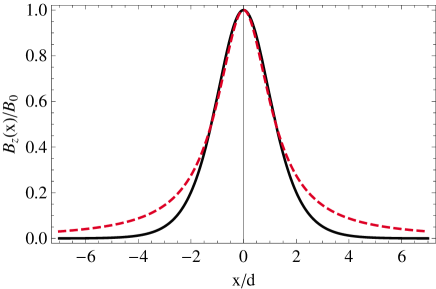
Figure 1: (color online) Magnetic field profile for the hyperbolic expression in Eq. (1) (solid line) as compared to the profile $B_{z}(x)=-(\mu_{0}M/4\pi)\ln[(x^{2}+k^{2})/(x^{2}+(l+h)^{2})]$, vancu:5074 produced by a ferromagnetic strip with a magnetization $\mu_{0}M$, thickness $l$ and separated a distance $h$ from the two dimensional system (dashed line). The parameters are selected in such a way that the peak and half width of both profiles have the same value.

here $\boldsymbol{e}_{z}$ is the unit vector normal to the graphene plane. This expression for the magnetic field presents several advantages: $(i)$ We obtain an analytically solvable model, that allows us to analyze in detail the bound spectra, as well as the transmission through the magnetic barrier. $(ii)$ In order to have conditions that are physically relevant to the study of graphene, we need a magnetic field $B(x)$ that varies slowly on the scale of the graphene lattice spacing, $a=0.246\,nm$. Selecting $a\ll d$, we observe that both the half-width ($\Lambda\approx 3.25\,d)$ and the edge smearing length $|(1/B)(dB/dx)|\sim d$ of the magnetic barrier satisfy the required conditions. $(iii)$ As shown in Fig.(1) the magnetic field in Eq. (1) provides a good approximation to the shape of the magnetic field barrier that is produced by a ferromagnetic film deposited on the top of a two dimensional system vancu:5074 . Thus the present formalism could be useful to analyze a similar arrange of inhomogeneous magnetic barriers in graphene samples.

The gauge can be selected in such a way that the vector potential is written as $\mathbf{A}=\hat{e}_{y}\,A(x)$ with

$$A(x)=2\,B_{0}\,d\,tanh\left(\frac{x}{2\,d}\right)\,.$$ (2)

Notice that if we consider that the system is confined within a square box of area $L\times L$, then in the $d>>L$ limit, the magnetic field can be consider homogeneous, and the vector potential reduces to the Landau gauge expression $\mathbf{A}=B_{0}\,(0,x,0)$.

On low energy scales the dynamics of quasiparticles in graphene is described by two independent 2+1 dimensional Dirac equations, the equations remain decoupled in the presence of smoothly varying magnetic field. The resulting time-independent Dirac equation describing low energy excitations around the $K$ point in the Brillouin zone is written as

$$H\,\psi(x,y)\,=\,v_{F}\vec{\sigma}\cdot\left[\mathbf{p}+e\mathbf{A}(x)\right]\,\psi(x,y)\,=\,E\psi(x,y)\,,$$ (3)

here the Fermi velocity is $v_{F}\approx c/300$, $\mathbf{p}=-i\hbar\nabla$ is the momentum operator and the isospin Pauli matrices $\sigma_{i}$ operate in the spinor $\psi(x,y)=\left(\psi_{A}\,,\,\psi_{B}\right)^{T}$, that represent the electron amplitude on two sites ($A$ and $B$) in the unit cell of the graphene lattice. Taking into account the translational invariance along the $y$ direction we seek solution of the form $\psi_{A}=exp(i{k_{y}\,y})\psi_{+}$ and $\psi_{B}=exp(i{k_{y}\,y})\psi_{-}$. The Dirac equation yields the coupled equations

$$\Delta\,\psi_{+}(x) = \left(-i\,\frac{\partial}{\partial{\tilde{x}}}-iW(x)\right)\psi_{-}(x)\,,$$

$$\Delta\,\psi_{-}(x) = \left(-i\,\frac{\partial}{\partial{\tilde{x}}}+iW(x)\right)\psi_{+}(x)\,,$$ (4)

with the magnetic length defined as $l_{B}=\sqrt{\hbar/eB_{0}}$, ${\tilde{x}}=x/l_{B}$, and $\Delta=E\,l_{B}/\hbar v_{F}$. The function $W(x)$ is given by

$$W(x)\,=\,l_{B}k_{y}+\frac{el_{B}A(x)}{\hbar}\,=\,l_{B}k_{y}+\frac{2d}{l_{B}}\tanh\left(\frac{x}{2\,d}\right)\,.$$ (5)

Combining the two equations in (II) we obtain the decoupled equations

$$H_{\pm}\,\psi_{\pm}(x)=\left(-\frac{d^{2}}{d{\tilde{x}}^{2}}+V_{\pm}\right)\,\psi_{\pm}(x)=\Delta^{2}\,\psi_{\pm}(x)\,,$$ (6)

where the effective potentials $V_{\pm}$ are given by

$$V_{\pm}(x)=W^{2}\pm\frac{dW}{d{\tilde{x}}}=\left[\left(l_{B}k_{y}+\frac{2d}{l_{B}}\,\tanh\left(\frac{x}{2\,d}\right)\right)^{2}\,\pm\,\,sech^{2}\left(\frac{x}{2\,d}\right)\right]\,.$$ (7)

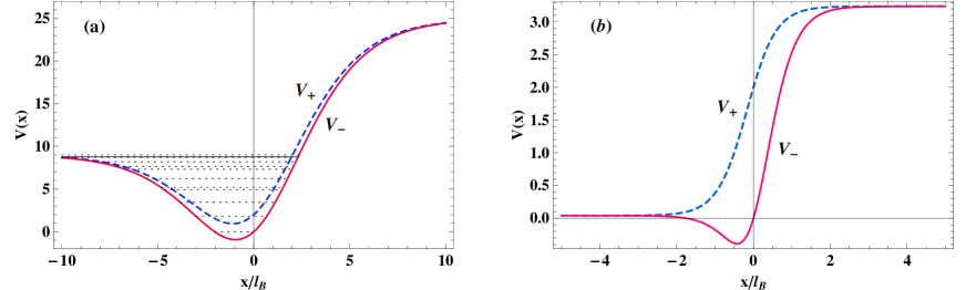
Figure 2: (color online) Plots of the effective potentials $V_{-}$ (solid lines) and $V_{+}$ (dashed lines) versus $x/l_{B}$. (a) The parameters $k_{y}l_{B}=1$, $d/l_{B}$ = 2 satisfy the condition in (18). The $\Delta^{2}(k_{y})$ eigenvalues are represented by the dotted lines. (b) $k_{y}l_{B}=1$, $d/l_{B}=0.4$, notice that in this case the condition in (18) is not satisfied, and therefore bounds states are not supported.

Both the shape and the depth of the effective potentials depend on the transverse momentum $k_{y}$. As seen in Fig.(2), depending on the values of $k_{y}$ and $d$, the effective potentials can assume the form of potential wells or steps. In next sections the bound state spectrum and scattering properties will be analyzed in detail.

It is interesting to point out that the Dirac equation in the presence of an external magnetic fields posses a formal structure that can be analyzed within the formalism of supersymmetric quantum mechanics (SUSY-QM) coop:267 ; coop:0 ; kuru:455305 . The potentials $V_{+}$ and $V_{-}$ in (7) are known as the super-partner potentials, they are obtained from the superpotential function $W(x)$ by the relation in (7). The explicit expressions for $V_{\pm}$ for the gauge potential in (2) are identified as the Rosen-Morse II potentials coop:267 ; coop:0 and the corresponding Schrödinger equations are exactly solvable. There are important property of SUSY-QM that relate the spectrum and eigenfunctions of the effective hamiltonians of $H_{+}$ and $H_{-}$ in Eq. (6). In particular, except from the ground state, $H_{+}$ and $H_{-}$ have the same spectrum for $\Delta^{2}$.

It is convenient to define the operators

$$L^{\pm}\,=\,-i\frac{d}{d{\tilde{x}}}\pm i\,W(x)\,.$$ (8)

In terms of these operators the relation between the upper and lower spinor components in (II) simply read

$$\,\psi_{+}(x)=\frac{1}{\Delta}L^{-}\psi_{-}(x)\,,\hskip 42.67912pt\,\psi_{-}(x)=\frac{1}{\Delta}L^{+}\psi_{+}(x)\,.$$ (9)

Let us introduce the dimensionless variable

$$\xi=\frac{1}{1+exp(x/d)}\,,$$ (10)

that varies from $0$ to $1$, as $x$ goes from $\infty$ to $-\infty$. In the new variable equations (6) become

$$\left[\frac{d^{2}}{d\xi^{2}}+\frac{1-2\xi}{\xi(1-\xi)}\frac{d}{d\xi}+\left(\frac{d}{l_{B}}\right)^{2}\frac{\Delta-\left[k_{y}l_{B}+2d/l_{B}(1-2\xi)\right]^{2}\pm 4\xi(1-\xi)}{\xi^{2}(1-\xi)^{2}}\right]\psi_{\pm}=0\,.$$ (11)

These equations have the asymptotic solutions: $\psi_{\pm}\sim\xi^{\rho}$ for $\xi\to 0$ ($x\to\infty$) and $\psi_{\pm}\sim(1-\xi)^{\sigma}$ for $\xi\to 1$ ($x\to-\infty$), where the asymptotic behavior is determined by

$$\rho\,=\,\frac{d}{l_{B}}\sqrt{\left(l_{B}\,k_{y}+\frac{2d}{l_{B}}\right)^{2}-\Delta^{2}}\,,\hskip 42.67912pt\sigma\,=\,\frac{d}{l_{B}}\sqrt{\left(l_{B}\,k_{y}-\frac{2d}{l_{B}}\right)^{2}-\Delta^{2}}\,.$$ (12)

In order to obtain consistent solutions, we recall that besides solving the effective Schrödinger equation in (11), the wave function components are interrelated by the Dirac equation via (9). Then, one can consider the following options: (a) Equation (11) is solved for the lower component $\psi_{-}$, the corresponding upper component $\psi_{+}$ is obtained from the first relation in (9). (b) Equation (11) is solved for the upper component $\psi_{+}$, and the lower component is obtained from the second relation in (9). We consider the first option, the second option gives equivalent solutions, except for the $n=0$ state. Taking into account the asymptotic behavior, we propose an ansatz of the form $\psi_{-}(\xi)=\xi^{\rho}(1-\xi)^{\sigma}f(\xi)$, substituting in Eq. (11) we find that $f(\xi)$ satisfies the Hypergeometric equation. Two linear independent solutions can be chosen as abra:00 : $f(\xi)=F\left(\alpha,\beta,\gamma;\xi\right)$ and $f(\xi)=\xi^{-2\rho}F\left(\alpha-\gamma+1,\beta-\gamma+1,2-\gamma;\xi\right)$; where $F\left(\alpha,\beta,\gamma;\xi\right)$ is the Hypergeometric function. However, the second solution has not the correct asymptotic behavior and has to be discarded. The corresponding upper component is obtained from the first equation in (9). The complete spinor solution is then given as

$$\psi=C\,e^{ik_{y}y}\xi^{\rho}\,\left(1-\xi\right)^{\sigma}\left(\begin{array}[]{c}\frac{il_{B}}{\Delta d}\,\left[G(\xi)\,F\left(\alpha,\beta,\gamma;\xi\right)+\xi(1-\xi)\frac{\alpha\beta}{\gamma}F\left(\alpha+1,\beta+1,\gamma+1;\xi\right)\right]\\ \\ F\left(\alpha,\beta,\gamma;\xi\right)\end{array}\right)\,,$$ (16)

where $G(\xi)\,=\,\left[(\rho-2d^{2}/l^{2}_{B})(1-\xi)-\xi(\sigma-2d^{2}/l^{2}_{B})-k_{y}d\right]$, $C$ is the normalization constant and

$$\alpha=\rho+\sigma-4\,\left(\frac{d}{l_{B}}\right)^{2}\,,\hskip 42.67912pt\beta=\rho+\sigma+4\,\left(\frac{d}{l_{B}}\right)^{2}+1\,,\hskip 42.67912pt\gamma=2\,\rho+1\,.$$ (17)

III Bound sates

Our aim is now to discuss the bound states spectrum. First we notice that the the electron-hole symmetry is preserved by the inhomogeneous magnetic field. This follow from the fact that the Hamiltonian in (3) anticommutes with the $\sigma_{3}$ matrix: $\{H,\sigma_{3}\}=0$. Then, if $\psi$ is an eigenvector of $H$ with eigenvalues $E$, $\sigma_{3}\psi$ is also an eigenvector with eigenvalue $-E$.

The fact that the Hamiltonians $H_{+}$ and $H_{-}$ share the same eigenvalues, implies that the existence of bound states requires that both $V_{+}$ and $V_{-}$ have the form of potential wells. This condition is obtained if the minima of $V_{\pm}$ are attained for a finite value of $x$, it is given by

$$l_{B}^{2}\,|k_{y}|<2\,d\,.$$ (18)

As seen in Fig.(2a), when the previous condition holds both $V_{+}$ and $V_{-}$ have the form of asymmetric potential wells around the guiding center position

$$x_{c}\,=\,2d\,arctanh\left(\frac{k_{y}}{2d}\right)\,.$$ (19)

Bounds states are found if the wells are sufficiently deep. In the limit in which the transverse momentum vanishes ($k_{y}=0$), the effective potentials reduce to symmetric wells centered at the maximum of $B(x)$. For values of $k_{y}$ in which the condition (18) is not obeyed at least one of $V_{\pm}$ take the form of a potential step Fig.(2b), and bounds states are not supported.

The solution in Eq. (16) leads to a divergence in $\xi\to 1(x\to-\infty)$ except for $\alpha$ or $\beta$ being a negative integer. Letting $\alpha=-n$, and utilizing Eq. (17) we obtain the energy spectrum, that can be conveniently written as

$$E_{n,k_{y}}=\pm\sqrt{2\hbar ev_{F}^{2}B_{0}}\sqrt{\left(n-\frac{(nl_{B})^{2}}{8d^{2}}\right)\left(1-\left(\frac{l_{B}^{2}k_{y}/2d}{1-n(l_{B}/2d)^{2}}\right)^{2}\right)}\,.$$ (20)

The index $n$ take the values $n=0,1,2,3.....n_{max}$. Both the allowed values of $n$ and and $k_{y}$ are restricted in order to satisfy the square integrability condition, explicitly they yield

$$n_{max}\leq 4\,\left(\frac{d}{l_{B}}\right)^{2}\,,\hskip 42.67912ptk^{d}_{y,\,max}\leq\,\frac{\left[4d^{2}-nl_{B}^{2}\right]^{2}}{8d^{3}\,l_{B}^{2}}\,.$$ (21)

The first condition determines the highest bound state supported for a given width of the barrier and eliminates the possible singularity in (20). Whereas, the second condition determines the allowed values of $k_{y}$ for a given $n$ and is related to the fact that the electron group velocity is limited by the free velocity in graphene, $i.e.$ $|\partial E_{n,k_{y}}/\partial p_{y}|\leq v_{F}$. The two conditions guarantee that $E_{n,k_{y}}\,<\,(\hbar v_{F}/l_{B})\,min\,\{V_{\pm}(\pm\infty)\}$, so the electron does not escape towards $\pm\infty$; equivalently the coefficients in (12) that determine the wave function asymptotic behavior satisfy $\rho\,,\,\sigma>0$.

The wave function for the zero energy level takes a simple form that can be obtained by solving the first equation in (II) when $\Delta=0$, it reads

$$\psi=C\,e^{ik_{y}y}e^{-k_{y}x}\left[Sech\left(\frac{x}{2d}\right)\right]^{4(d/l_{B})^{2}}\,\left(\begin{array}[]{c}0\\ \\ 1\end{array}\right)\,.$$ (25)

Whereas, for other values of $n$ the Hypergeometric functions become Jacobi polynomials with energy dependent indices, the wave function is given by

$$\psi=Ce^{ik_{y}y}(1+z)^{\rho}\,\left(1-z\right)^{\sigma}\,\left(\begin{array}[]{c}\frac{il_{B}}{2\Delta d}\,\left[M(z)\,P_{n}^{(\gamma-1,-n+\beta-\gamma)}(z)-(1-z^{2})\,\frac{\alpha\beta}{2n}\,P_{n}^{(\gamma-1,1-n+\beta-\gamma)}(z)\right]\\ \\ P_{n}^{(\gamma-1,-n+\beta-\gamma)}(z)\end{array}\right)\,,$$ (29)

where $z=2\xi-1=tanh(x/2)$ and $M(z)\,=(\rho-2d^{2}/l^{2}_{B})(1-z)-(\sigma-2d^{2}/l^{2}_{B})(1+z)-2k_{y}d$.

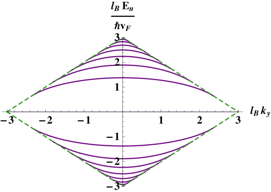
Figure 3: (color online) Bound states energy spectrum $E_{n}(k_{y})$ as a function of $k_{y}$ for a magnetic barrier with $d=1.5\,l_{B}$. According to (21) $n_{max}=9$. For every $n-$level the allowed values of $k_{y}$ are delimited by the free-electron spectrum $E=\pm\hbar v_{F}k_{y}$ (dashed lines).

The dispersion relation in (20) shows that the inhomogeneity of $B$ lifts the degeneracy for every quantum level $n$ and gives rise to a $k_{y}$-dependent dispersion relation, which leads to a drift velocity along the $y$ axis. This is valid, except for the $n=0$ level that has zero energy, independent on the magnetic field for all values of $k_{y}$. The energy spectrum for $d=1.5l_{B}$ is displayed in Fig.(3) as a function of $k_{y}$. For the selected values we have $n_{max}=9$, and each level $n$ results in a band as the transverse momentum sweeps from $k_{y}=0$ to the maximum value $k_{y,max}^{d}$ in (21).

The previous results apply when the width of the barrier is small in comparison with the system dimensions. We now analyze the behavior of the spectrum as we change from a narrow to a broad barrier, considering that the system is confined within a square box of length $L\times L$. For a narrow barrier the values of $k_{y}$ are limited by the second equation in (21). Instead, when the size of the barrier is comparable to $L$, the number of allowed states is limited by those that can be accommodated in the square box. Assuming periodic conditions for the wave function in (29) along the $y-$direction, yield $k_{y}=2\pi\,j/L$ with $j$ an integer. But according to Eq. (19) $k_{y}$ also determines the center position $x_{c}$ of the electron, hence $x_{c}<L/2$ and the number of quantum states is given by $N=j_{max}=(2dL/\pi l_{B}^{2})\tanh\left(L/4d\right)$, whereas the momentum limit imposed by the size of the system reads $k^{L}_{y,\,max}=2(d/l_{B}^{2})\tanh\left(L/4d\right)$. It is interesting to notice, that similarly to the homogeneous case, the degeneracy can be written as $N=\Phi/\Phi_{0}$, where the magnetic flux produced by the field in (1) through the sample is $\Phi=4B_{0}dL\tanh\left(L/4d\right)$ and $\Phi_{0}=h/e$ is the elementary fluxon. In order to track the degeneracy evolution as the barrier is modified from narrow to broad as compared to $L$, we define

$$\frac{1}{K_{y,\,max}}=\frac{1}{k^{L}_{y,\,max}}+\frac{1}{k^{d}_{y,\,max}}\,$$ (30)

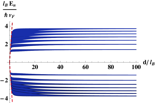
Figure 4: (color online) Energy spectrum as a function of $d$ for a magnetic barrier when the system is confined by a square box of area $L\times L$ with $L=50l_{B}$. The dark zones are the allowed energy values. The dashed line $El_{B}/\hbar v_{F}=2d/l_{B}$ delimitates the minimum barrier width that supports bound states. For every level $n$ the transverse momentum varies between $k_{y}=0$ and $k_{y}=K_{y,\,max}$.

as a cut for the transverse momentum. Notice that $K_{y,\,max}$ interpolates between $k^{d}_{y\,max}$ valid for a narrow barrier, and $k^{L}_{y,\,max}$ valid when $d>L$. Fig.(4) shows the resulting energy spectrum, the dark zones are the allowed energy values. For every level $n$ the transverse momentum varies between $k_{y}=0$ and $k_{y}=K_{y,\,max}$. The restriction on the level index $n$ given by the first equation in (21), translates into the following equation for the separatrix $E=2\hbar v_{F}d/l^{2}_{B}$ (dashed line), energies to the left of this line are not allowed. For small value of $d/l_{B}$ a few bands and gaps can be identified for the first values of $n$, as the energy is increased we observe a continuous energy region up to the maximum allowed value $n_{max}$. As the size of the barrier increases a larger number of energy gaps appear. When the size of the magnetic barrier becomes comparable to $L$ the width of the bands decrease. Finally in the homogeneous $B$ limit, $d\gg L$, the energy eigenvalues reduce to the relativistic massless Landau levels observed in graphene: $E_{n,k_{y}}=\pm\sqrt{2\hbar ev_{F}^{2}B_{0}\,n}$, independently of $k_{y}$, whereas the degeneracy reduces to the well known result $N=\Phi/\Phi_{0}$, with $\Phi=B_{0}L^{2}$.

IV Scattering

We now consider the scattering regime. A plane wave incident from $x\to-\infty\,,(\xi\to 1)$ propagates at an angle $\phi$ with respect to the $x$ axis. Taking into account the gauge selection in (2) the incoming momenta are parametrized as

$$l_{B}\,k_{x}=\Delta\cos\phi\,,\hskip 42.67912ptl_{B}\,k_{y}=\Delta\sin\phi+\frac{2d}{l_{B}}\,.$$ (31)

The transmitted wave has a longitudinal momentum $k_{x}^{\prime}=\frac{\Delta}{l_{B}}\cos\phi^{\prime}$ where $\phi^{\prime}$ is the refracted angle. The conservation of $k_{y}$ gives the relation between the incident and refracted angle as follows

$$\sin\phi^{\prime}=\sin\phi+\frac{4\,d}{l_{B}\,\Delta}\,,$$ (32)

whereas energy conservation allow us to relate the transmitted and incident longitudinal momenta as

$$l_{B}\,k_{x}^{\prime}=\sqrt{\left(l_{B}\,k_{x}\right)^{2}-\ \left(\frac{4d}{l_{B}}\right)^{2}-8k_{y}d}\,.$$ (33)

Eq. (32) implies that for a critical angle $\phi_{c}=\arcsin\left(1-4d/l_{B}\Delta\right)$ no transmission is possible. Furthermore, when the following condition applies

$$\frac{El_{B}}{\hbar v_{F}}\,\leq\,2\,\frac{d}{l_{B}}\,,$$ (34)

the transmission vanishes regardless of the incident angle $\phi$. The condition in (34) establish that states with an average cyclotron radius (in the barrier region) smaller that $2d$ will bend by the magnetic field and are completely reflected, a similar condition was obtained in the case of a square-well magnetic barrier mart:066802 . Comparing the equations (31) with (12), we observe that the longitudinal momenta $k_{x}$ and $k_{x}^{\prime}$ are related to the asymptotic coefficients $\rho$ and $\sigma$ as follows: $\sigma=-ik_{x}\,d$ and $\rho=d\,\sqrt{-k_{x}^{\prime 2}}$. It is verified that if condition (34) holds $\rho$ is real, instead when (34) is not valid we replace $\rho=-ik_{x}^{\prime}\,d$. Utilizing the properties of the Hypergeometric functions it is verified that in the limit $x\to\infty\,(\xi\to 0)$ the wave function in (16) yields the correct asymptotic expression

$$\psi\sim\,e^{i(k_{x}^{\prime}x+k_{y}y)}\,\left(\begin{array}[]{c}s\,e^{-i\phi^{\prime}}\\ \\ 1\end{array}\right)\,,$$ (38)

where $s=sgn\,E$. The asymptotic value of the wave function for $x\to-\infty\,(\xi\to 1)$, is obtained using the linear transformation formulasabra:00 that relate $F(\alpha,\beta,\gamma,\xi)$ with Hypergeometric functions evaluated at $1-\xi$, to obtain

$$\psi\sim\,e^{i(k_{x}x+k_{y}y)}\,\frac{\Gamma\left(\gamma\right)\Gamma\left(\gamma-\alpha-\beta\right)}{\Gamma\left(\gamma-\alpha\right)\Gamma\left(\gamma-\beta\right)}\,\left(\begin{array}[]{c}s\,e^{i\phi}\\ \\ 1\end{array}\right)\,\,+\,\,\,e^{i(-k_{x}x+k_{y}y)}\,\frac{\Gamma\left(\gamma\right)\Gamma\left(\alpha+\beta-\gamma\right)}{\Gamma\left(\alpha\right)\Gamma\left(\beta\right)}\left(\begin{array}[]{c}-s\,e^{-i\phi}\\ \\ 1\end{array}\right)\,.$$ (45)

From this equation the reflection coefficient $R$ is obtained as

$$R=\Bigg{|}\frac{\Gamma\left(\rho-ik_{x}d+(2d/l_{B})^{2}+1\right)\Gamma\left(\rho-ik_{x}d-(2d/l_{B})^{2}\right)}{\Gamma\left(\rho+ik_{x}d+(2d/l_{B})^{2}+1\right)\Gamma\left(\rho+ik_{x}d-(2d/l_{B})^{2}\right)}\Bigg{|}^{2}\,.$$ (46)

Under condition (34) $\rho$ is real, thus $R=1$ and, as expected, the transmission coefficient vanishes. Instead, if the condition (34) is not obeyed, $\rho$ is substituted by $\rho=-idk_{x}^{\prime}$, and the transmission probability $T=1-R$ can be written in a simple closed form as

$$T\,=\,\frac{\sinh\left[2\pi l_{B}k_{x}\right]\,\sinh\left[2\pi l_{B}k_{x}^{\prime}\right]}{\sin^{2}\left[4\pi\left(\frac{d}{l_{B}}\right)^{2}\right]\,+\,\sinh^{2}\left[\pi l_{B}(k_{x}+k_{x}^{\prime})\right]}\,.$$ (47)

A plot for the transmission coefficient as a function of the incidence angle is shown in Fig.(5) for a fixed energy and several values of $d$. The qualitative behavior in this plot is similar to those obtained for the case of a square well magnetic barrier mart:066802 . However an advantage of the the result in (47) is that it allow us to identify the resonant conditions at which the barrier becomes transparent ($T\sim 1$), it is given by

$$d=\frac{\sqrt{j}}{2}\,l_{B}\,\hskip 42.67912ptj=1,2,3,.....$$ (48)

In this case the barrier acts as an asymmetric filter, it behaves as perfectly transparent for angles in the region $-\pi/2<\phi<\phi_{c}$ Fig.(6a). In particular for energy values slightly above the threshold condition in (34), $\Delta=d/l_{B}+\epsilon$, with $\epsilon\ll 1$, the width of the transparency region can be very narrow.

On the other hand, under the condition

$$d=\frac{\sqrt{j+\frac{1}{2}}}{2}\,l_{B}\,\hskip 42.67912ptj=0,1,2,3,.....$$ (49)

the value of $T$ is reduced, in particular for values of the energy slightly above the threshold condition in (34), $\Delta=d/l_{B}+\epsilon$, with $\epsilon\ll 1$, the transmission coefficient is strongly reduced, Fig.(6b). Another way to contrast these results is shown in Fig.(7) where a contour plot for the transmission coefficient $T$ is shown. A can be seen in Fig.(7(a) corresponding to the resonant condition in Eq. (48) there is a wider region for the transmission that is not present in Fig.(7(b) corresponding to the minima condition in Eq. (49).

V Conclusions

In conclusion, we consider the dynamics of carriers in graphene subjected to an inhomogeneous hyperbolic magnetic field. The corresponding Dirac equations was analyzed within the formalism of supersymmetric quantum mechanics. We found compact analytical solutions for the energy eigenvalues and eigenfunctions for electrons and holes. The dispersion relation in (20) shows that the inhomogeneity of $B$ lifts the degeneracy for every quantum level $n$ and gives rise to a $k_{y}$-dependent dispersion relation, which leads to a drift velocity along the $y$ axis. This is valid, except for the $n=0$ level that has zero energy, independent on the magnetic field for all values of $k_{y}$. For a narrow barrier the spectra displays a series of bands separated by gaps, as the width of the barrier increases we can track the levels evolution into the degenerated Landau levels. In the scattering regime a simple analytical formula is obtained for the transmission coefficient, this result allow us to identify the resonant conditions at which the barrier becomes transparent. We expect that the results obtained in this work will be useful in order to analyze the confinement by magnetic barriers in graphene samples. In a future work we plan to address the problem of calculating the longitudinal conductivity as well as the Hall conductivity for the case of graphene under inhomogeneous magnetic fields.

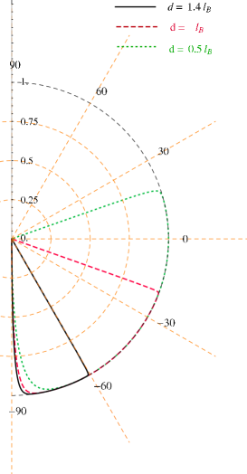
Figure 5: (color online) Angular dependence of the transmission coefficient $T$ through a barrier with energy $\Delta=El_{B}/\hbar v_{F}=3$ and different values for $d$: $d=1.4l_{B}$ (continuos line), $d=l_{B}$ (dashed line), and $d=0.5l_{B}$ (dotted line).

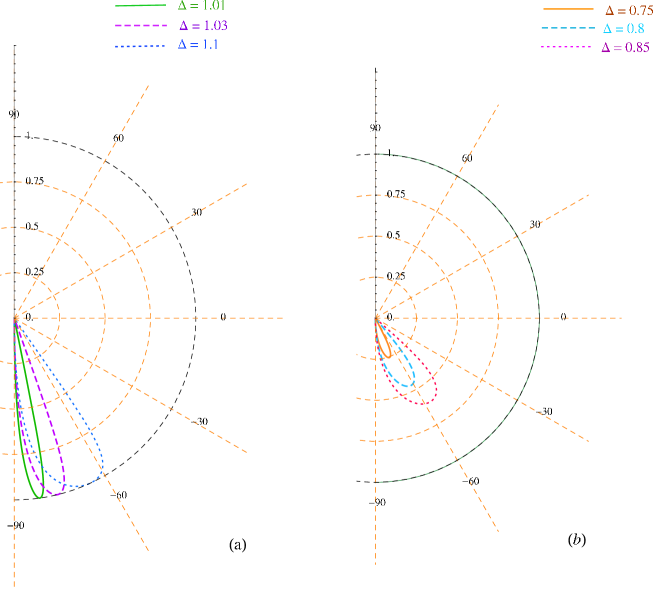
Figure 6: (color online) (a) Angular dependence of the transmission coefficient $T$ through a barrier with $d=l_{B}/2$ (resonant condition in Eq. (48) with $j=1$), and the following values of the energy: $\Delta=1.01$ continuos line, $\Delta=1.03$ dashed line, and $\Delta=1.1$ dotted line. (b) As in (a) for $d=l_{B}/\sqrt{8}$ (Eq. (49) with $j=0$) and the following values of the energy: $\Delta=0.75$ (continuos line), $\Delta=0.8$ (dashed line), and $\Delta=0.85$ (dotted line).

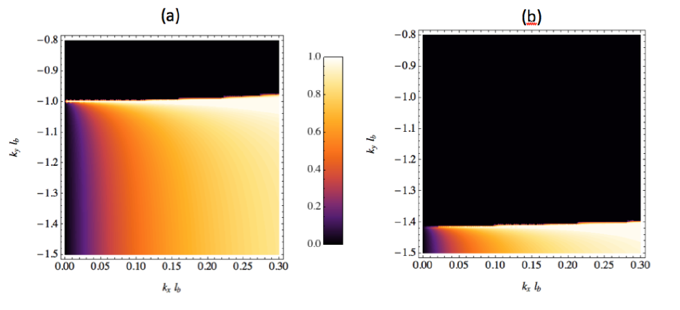
Figure 7: (color online) a) Contour plot of the transmission coefficient $T$ through a barrier with $d=l_{B}/2$ (resonant condition in Eq. (48) with $j=1$), (b) As in (a) for $d=l_{B}/\sqrt{8}$ (Eq. (49) with $j=0$).

- (1) K. Novoselov, A. Geim, S. Morozov, D. Jiang, Y. Zhang, S. Dubonos, I. Grigorieva, and A. Firsov, Science 306, 666 (2004).
- (2) K. Novoselov, A. Geim, S. Morozov, D. Jiang, M. Katsnelson, I. Grigorieva, S. Dubonos, and A. Firsov, Nature 438, 197 (2005).
- (3) Y. Zhang, Y. Tan, H. Stormer, and P. Kim, Nature 438, 201 (2005).
- (4) M.I. Katsnelson, Materials Today 10, 20 (2007).
- (5) K. S. Novoselov, Z. Jiang, Y. Zhang, S. V. Morozov, H. L. Stormer, U. Zeitler, J. C. Maan, G. S. Boe- binger, P. Kim, and A. K. Geim, Science 315, 1379 (2007).
- (6) K. S. Novoselov, E. McCann, S. V. Morozov, V. I. Fal ko, M. I. Katsnelson, U. Zeitler, D. Jiang, F. Schedin, A. K. Geim, Nature Physics 2, 177 (2006).
- (7) P.R. Wallace, Phys. Rev 71, 622 (1947).
- (8) G.W. Semenoff, Phys. Rev. Lett. 53, 2449 (1984).
- (9) A. H. Castro Neto, F. Guinea, N. M. R. Peres, K. S. Novoselov, and A. K. Geim, Rev. Mod. Phys. 81, 109 (2009).
- (10) K. Ziegler, Phys. Rev. B 75, 233407 (2007).
- (11) V. P. Gusynin, and S. G. Sharapov, Phys. Rev. Lett. 95, 146801 (2005).
- (12) M.I. Katsnelson, K. S. Novoselov, and A. K. Geim, Nature Phys. 2, 620 (2006).
- (13) V. V. Cheianov, and V. I. Fal’ko Phys. Rev. B 74 , 041403 (R) (2006).
- (14) M.I. Katsnelson, European Phys. J. B 51, 157 (2006).
- (15) A. F. Young, and P. Kim, Nature Phys. 5, 222 (2009).
- (16) A. De Martino, L. Dell’ Anna, and R.Egeger, Phys. Rev. lett. 98, 066802 (2007).
- (17) M. Ramezani Masir, P. Vasilopoulos, A. Matulis, and F. M. Peeters, Phys. Rev. B 77, 235443 (2008).
- (18) L. Dell’ Anna, and A. De Martino, cond-mat,mes-hall/1101.1918v1 (2011).
- (19) L. Oroszlany, P. Rakyta, A. Kormanyos, C. J. Lambert, and J. Csert, Phys. Rev. B 77, 081403 (R) (2008).
- (20) S. J. Lee, S. Souma, G. Ihm, and K. J. Chang, Phys. Rep. 394, 1 (2004).
- (21) T. Vancura, T. Ihn, S. Broderick, K. Ensslin, W. Wegscheider, and M. Bichler, Phys. Rev. B 62, 5074 (2000).
- (22) H. A. Carmona, A. K. Geim, A. Nogaret, P. C. Main, T. J. Foster, and M. Henini, Phys. Rev. Lett. 74, 3009 (1995).
- (23) P. D. Ye, D. Weiss, R. R. Gerhardts, M. Seeger, K. von Klitzing, K. Eberl, and H. Nickel, Phys. Rev. Lett. 67, 3013 (1995).
- (24) K. S. Novoselov, A. K. Geim, S. V. Dubonos, Y. G. Cornelissens, F. M. Peeters, and J. C. Maan, Phys. Rev. B 65, 233312 (2002).
- (25) F. M. Peeters, and A. Matulis Phys. Rev. B 48, 15166 (1993).
- (26) A. Matulis, F. M. Peeters, and P. Vasilopoulos, Phys. Rev. Lett. 72, 1518 (1994).
- (27) K. Handrich, Phys. Rev. B 72, 161308 (R) (2005).
- (28) F. Cooper, A. Khare, and U. Sukhatme, Phys. Rep. 251, 267 (1995).
- (29) F. Cooper, A. Khare, and U. Sukhatme, “Supersymmetry in Quantum Mechanics”, World Scientific, Inc. Singapore, New Jersey, London, and Hong Kong (2001).
- (30) S. Kuru, J. Negro, and L. M. Nieto, J. Phys. Cond. Matter 21, 455305 (2009).
- (31) M. Abramowitz, I. A. Stegun, “Handbook of mathematical functions”, Dover Publications, Inc. New York (1972).