Modeling the Dispersal of an Active Region: Quantifying Energy Input into the Corona

Abstract

In this paper a new technique for modeling non-linear force-free fields directly from line of sight magnetogram observations is presented. The technique uses sequences of magnetograms directly as lower boundary conditions to drive the evolution of coronal magnetic fields between successive force-free equilibria over long periods of time. It is illustrated by applying it to MDI observations of a decaying active region, NOAA AR 8005. The active region is modeled during a 4 day period around its central meridian passage. Over this time, the dispersal of the active region is dominated by random motions due to small scale convective cells. Through studying the build up of magnetic energy in the model, it is found that such small scale motions may inject anywhere from $2.5-3\times 10^{25}$ ergs s^-1 of free magnetic energy into the coronal field. Most of this energy is stored within the center of the active region in the low corona, below 30 Mm. After 4 days the build-up of free energy is 10$\%$ that of the corresponding potential field. This energy buildup, is sufficient to explain the radiative losses at coronal temperatures within the active region. Small scale convective motions therefore play an integral part in the energy balance of the corona. This new technique has wide ranging applications with the new high resolution, high cadence observations from the SDO:HMI and SDO:AIA instruments.

1 Introduction

The solar corona is a complex environment, where much of its complexity is due to magnetic fields. These magnetic fields are produced through a dynamo action near the base of the convection zone (Charbonneau, 2005). Once formed they may become buoyantly unstable, rise through the convective zone and break through the photosphere (Archontis et al., 2004; Magara, 2004; Galsgaard et al., 2007; Murray & Hood, 2008; Fan, 2009) where they are observed as either sunspots in white light or active regions in magnetograms. Such active regions structure the Sun’s atmosphere and provide energy for eruptive phenomena such as solar flares (Benz, 2008) and CMEs (Cremades et al., 2006).

Once active regions form, small scale motions such as granular and supergranular flows result in the decay of the active region and the dispersal of magnetic flux across the solar surface in a random walk (Leighton, 1964). This random walk leads to the convergence and cancellation of magnetic flux along Polarity Inversion Lines (PILs), in addition to the spreading of magnetic fields. Such evolution of magnetic elements in the photosphere acts as a driver for the build up of free magnetic energy in the solar corona. The subsequent evolution of the coronal field through quasi-static equilibria, in response to these motions, may be mathematically modeled through force-free magnetic fields, magnetic fields which satisfy $\bf{j}\times\bf{B}=0$ where ${\bf j}=\alpha{\bf B}$ (Priest, 1982).

In recent years, non-linear force-free field modeling has received much attention (Schrijver et al., 2006; Metcalf et al., 2008). A non-linear force-free field, is a special class of force-free field, where the scalar function $\alpha(r)$ is a function of position, but must be constant along any field line. Non-linear force-free fields are of particular interest as they may contain free magnetic energy (Woltjer, 1958). The construction of non-linear force-free fields (NLFFF) may be broadly split into two groups: static and time-dependent models. Examples of static modeling are the “extrapolation” of photospheric vector magnetic fields into the corona (Schrijver et al., 2006; Regnier & Priest, 2007; De Rosa et al., 2009; Wheatland & Régnier, 2009; Jing et al., 2010), and direct fitting of NLFFF models to observed filaments and coronal structures (van Ballegooijen, 2004; Bobra et al., 2008; Su et al., 2009b; Savcheva & van Ballegooijen, 2009). Static modeling involves constructing either individual NLFFFs or independent sequences of magnetic configurations, where there is no direct correlation or evolution between the different fields.

In contrast, time-dependent quasi-static modeling evolves the coronal magnetic field through continuous sequences of related non-linear force-free fields based on the evolution of a continuous time dependent lower boundary condition. This boundary condition may be specified through either idealized magnetic field configurations (van Ballegooijen et al., 2000; Mackay & Gaizauskas, 2003; Mackay & van Ballegooijen, 2005, 2006a, 2009) or from observations (Mackay et al., 2000; Yeates et al., 2007, 2008). Only through using dynamic models can the build up of free magnetic energy and magnetic helicity in the corona be studied, along with the evolution of isolated flux and current systems. Such a technique has been successfully applied in the past to model the evolution of the global corona (Mackay & van Ballegooijen, 2006a, b; Yeates & Mackay, 2009), determine the origin and evolution of solar filaments (Yeates et al., 2008; Mackay & van Ballegooijen, 2009), study the formation and lift off of magnetic flux ropes (Mackay & van Ballegooijen, 2006b; Yeates & Mackay, 2009; Yeates et al., 2010) and finally the origin of the Sun’s Open Magnetic Flux (Mackay & van Ballegooijen, 2006b; Yeates et al., 2010).

In this paper we apply time dependent quasi-static non-linear force-free modeling to model the effect that the dispersal of an active region has on the overlying coronal magnetic field. A key difference between this paper and previous studies is the manner in which the time dependent lower boundary condition is applied. In previous studies either idealized magnetic field distributions or simplified surface configurations derived from observations were prescribed. In the present study, a new technique of prescribing the time dependent lower boundary condition is presented. The technique allows the use of observed line of sight component magnetograms directly as lower boundary conditions, reproducing as observed, the dispersal of the photospheric flux of the active region. From this the effect of the surface motions on the coronal magnetic field and the subsequent energy input into the corona is determined.

The active region chosen to illustrate this new technique is NOAA AR 8005. It is chosen as it was an isolated region and during the period of observations there appears to be no significant flux emergence and the flux is well balanced throughout. The structure of the paper is as follows. In Section 2 the main properties of the decaying active region are discussed. In Section 3 the modeling technique for both the photospheric and coronal fields are described. The results of the simulation are given in Section 4, while in Section 5 some simple calculations are compared to the simulations to verify the results. Finally a discussion and conclusions are given in Section 6.

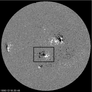
Figure 1: SoHO MDI $96$ min line of sight component magnetogram for 18^th Dec 1996 where white represents positive magnetic polarities and black negative magnetic polarities. The active region of interest, NOAA 8055, lies in the southern hemisphere at central meridian and is enclosed by the black box.

2 Observations

The decaying active region considered in this study is NOAA AR 8005. It emerged on the far side of the Sun and as it rotated onto the limb only dispersed magnetic polarities, without sunspots were present. In Figure 1 a full disk SOHO:MDI (Scherrer et al., 1995) $96$min line of sight component magnetogram from 18^th Dec 1996 can be seen. The active region of interest lies at central meridian just below the equator. It has a simple magnetic morphology with a single positive and negative polarity.

To study the evolution of the active region, SoHO:MDI $96$min magnetograms are obtained from 19.12.05 UT on 16^th December 1996 to 20.47.05 UT on 20^th December 1996, spanning a period of four days. The four day period was chosen to include, two days before and two days after central meridian passage, which occurs late on 18^th December. During this period as LOS projection effects are minimized, the measurements of the magnetic flux are known to be the most reliable. In total 61, $96$ min magnetograms cover the period of interest. The data are corrected for the area foreshortening that occurs away from central meridian using the IDL Solar Software routine drot_map. An area of $181\times 126$ pixels is cut out of the rotated magnetograms centered on NOAA 8055 where each pixel is $1.977^{\prime\prime}$. A time sequence of these can be seen in Figure 2. The area was chosen to be large enough to encompass the whole active region, but small enough that approximate flux balance is achieved. The active regions that lie to the north and south of NOAA 8005 have no contribution to the flux in the area considered.

On studying the magnetograms over the period of interest, the evolution of NOAA 8005 is dominated by the dispersal of magnetic flux from the main flux concentrations. There is no significant emergence of new magnetic bipoles. On studying Figure 2 or the movie of the evolution (movie1.mpg), the motion of the magnetic elements is clearly dominated by a random walk due to supergranular flows and no strong shear or vortical flows are present. In Figure 3 the separation distance ($S(t)$) between the centers of flux in both the positive and negative polarities can be seen, given as a function of time ($t$). This separation is defined as $S=\mid{\bf{S}}(t)\mid$ where ${\bf{S}}(t)$ is the vector pointing between the centers of flux in each polarity,

$${\bf{S}}(t)=\frac{\sum_{B_{z}>0}B_{z}(i,j){\bf{R}}_{i,j}}{\sum_{B_{z}>0}B_{z}(i,j)}-\frac{\sum_{B_{z}<0}B_{z}(i,j){\bf{R}}_{i,j}}{\sum_{B_{z}<0}B_{z}(i,j)}$$ (1)

where $B_{z}(i,j)$ is the line of sight component of the field at the $i^{th}$,$j^{th}$ pixel and ${\bf{R}}_{i,j}$ is the position vector of the i^th,j^th pixel from the origin. The origin is defined to be the lower left corner of the magnetogram. Throughout the four day period, as the active region crosses central meridian, the separation of the polarities is seen to slightly increase from $68,000$km to $80,000$km. This increase is only $18\%$ that of the initial separation. While in general, the region is diverging, there are several instances where patches of strong magnetic flux separate from the main polarities and cancel along the Polarity Inversion Line. A key point to note is that during the evolution no systematic shear motions or vortical motions of the magnetic flux are seen. The motions of magnetic elements are mainly due to the buffeting as a result of supergranular motions. Although supergranular motions provide the only obvious flow pattern, due to the large latitudinal extent of the active region differential rotation may have a small non-negligible effect. The evidence and consequences of this will be discussed in Section 6.

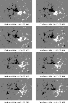
Figure 2: Time sequence of de-rotated SoHO MDI $96$ min line of sight component magnetograms of NOAA 8005. The time sequence covers the evolution of the active region 2 days before and 2 days after central meridian passage (18^th Dec 1996) where white represents positive magnetic polarities and black negative magnetic polarities. The images show the active region after it has been corrected for flux balance.

In Figure 4(a) the variation of the total unsigned magnetic flux within the selected active region can be seen as a function of time. The flux values are given in units of $10^{22}$Mx and time in days from 16^th December 1996 19.12.05 UT. The solid line in Figure 4(a) shows the total unsigned flux as derived from the individual magnetograms. The flux values are consistent with a medium sized active region. Initially over the first day the flux values are seen to increase slightly, possibly due to LOS changes as the region rotates toward central meridian and the emergence of a small bipole on the south-western edge of the active region. However, between days 1-4 the flux decays away as cancellation becomes significant along the internal PIL (Green & Kliem, 2009). By the end of day 4 the flux has dropped by $20\%$ of its original value. This behavior fits well with the observation that it is a decaying active region. The peak flux densities found within both the positive and negative polarities are around $1$kG. In Figure 4(b) the flux difference (flux imbalance) calculated for each magnetogram can be seen as a function of time. Over the four day period the imbalance is systematically negative, possibly due to a dominantly negative surrounding small scale fields. At worst it is $10\%$ that of the total flux of the active region. As this value is small, the active region may be regarded to be in flux balance to a high degree of accuracy.

To use the magnetograms as a lower boundary condition in the numerical simulations complete flux balance is required. Therefore in each magnetogram the imbalance per pixel is determined and subtracted from each pixel. This correction varies from one magnetogram to the next. In general it is less than $\mid 6\mid$G and so is comparable to the noise level within the magnetograms and significantly less that the peak flux density. After correction, the variation of the total unsigned flux is given by the dotted line in Figure 4(a). It can be seen that this line follows the uncorrected flux very closely and applying the correction does not significantly effect the net flux of the active region.

Figure 3: Separation between the center of flux of the positive and negative polarities as a function of time in days from 16^th December 1996 19:12 UT.

Figure 4: (a) Total unsigned flux ($10^{22}$Mx) as a function of time (days). The solid line denotes the value determined from the de-rotated data. The dashed line is once a correction has been applied to ensure flux balance. (b) Imbalance of flux ($10^{20}$Mx) as a function of time (days). In both panels, time is from 16^th December 1996 19:12 UT.

3 The Model

3.1 Coronal Model

To simulate the evolution of the coronal magnetic field above the active region a magnetofrictional relaxation technique is applied. This technique evolves the coronal magnetic field through a sequence of related non-linear force-free equilibria. The technique is similar to that described in the papers of van Ballegooijen et al. (2000) and Mackay & van Ballegooijen (2006a) where the code described in these papers is adapted to a local cartesian frame of reference. Previously the technique has been successfully applied to consider the coronal field based on evolving photospheric boundary conditions in either idealized setups (Mackay & Gaizauskas, 2003; Mackay & van Ballegooijen, 2005, 2009) or approximations to observed magnetograms (Mackay et al., 2000; Yeates et al., 2007, 2008). A key element of these simulations is that through considering a time sequence of evolved equilibria, this allows the memory of previous flux connectivities and currents to be maintained from one time to the next as energy and magnetic helicity is injected into the corona. Such a feature is significantly different compared to independent extrapolations which do not maintain such memory.

Figure 5: Field line plot showing the initial potential field used in the simulation. The thin solid/dashed lines denote positive/negative contours of the normal field component on the base, while the thick lines are the field lines.

The magnetic field, ${\bf B}=\nabla\times{\bf A}$, is evolved by the induction equation,

$$\frac{\partial{\bf{A}}}{\partial t}={\bf{v}}\times{\bf{B}}$$ (2)

where ${\bf{v}}({\bf{r}},t)$ is the plasma velocity and for the present study non-ideal terms are not included. To ensure that the coronal field evolves through a series of force-free states a magneto-frictional method is employed (Yang et al., 1986). We assume that the plasma velocity within the interior of the box (representing the solar corona) is given by,

$${\bf{v}}=\frac{1}{\nu}\frac{{\bf{j}}\times{\bf{B}}}{B^{2}},$$ (3)

where ${\bf{j}}=\nabla\times{\bf{B}}$ and $\nu$ is the coefficient of friction. Equation (3) represents in an approximate manner, the fact that in the corona the Lorentz force is dominant and simulates the plasma experiencing a frictional force as it moves with respect to the reference frame. This ensures that as the coronal field is perturbed via boundary motions it evolves through a series of quasi-static non-linear force-free field distributions, satisfying ${\bf{j}}\times{\bf{B}}=0$. To carry out the computations a staggered grid is used to obtain second order accuracy for all derivatives and closed boundary conditions are applied on the side and top boundaries to match those given in Section 3.2.

A key new feature within this study is that the evolution of the coronal field is driven directly through the insertion of a time sequence of observed line of sight component magnetograms. This means that the evolution of the photospheric field occurs in exactly the same way as is seen in the observations. No simplifications, idealization or smoothing is applied to the observed data and the data is inserted as observed (with only a small correction for flux balance applied). The technique of specifying the sequences of the lower boundary conditions is discussed next.

3.2 Lower Boundary Condition and Initial Condition

To model the evolution of the active region, 61 magnetograms taken at discrete intervals of $96$ min are available, covering the four day period around central meridian passage. From these magnetograms a continuous time sequence of lower boundary conditions is produced. This sequence of lower boundary conditions is designed to match each observed magnetogram, pixel by pixel, every 96 minutes. However, to model the evolution of the coronal field, $A_{xb}$ and $A_{yb}$ the horizontal components of the vector potential A on the base that correspond to this magnetogram must be determined. To determine these and produce a continuous time sequence the following process is applied,

1. Each of the observed magnetograms, $B_{z}(x,y,k)$ for $k=1\rightarrow 61$ are taken, where $k$ represents the discrete 96 min time index.

2. Next the horizontal components of the vector potential at the base, $z=0$, are written in the form,

   $$A_{xb}(x,y,k)=\frac{\partial\Phi}{\partial y},$$

   $$A_{yb}(x,y,k)=-\frac{\partial\Phi}{\partial x}$$

   where $\Phi$ is a scalar potential.

3. For each discrete time index $k$, the equation

   $$B_{z}=\frac{\partial A_{yb}}{\partial x}-\frac{\partial A_{xb}}{\partial y}$$

   then becomes,

   $$\frac{\partial^{2}\Phi}{\partial x^{2}}+\frac{\partial^{2}\Phi}{\partial y^{2}}=-B_{z}.$$ (4)

   which is solved using a multigrid numerical method. Details of this method can be found in the papers by Finn et al.(1994) and Longbottom (1998) and references therein. For a full description of the boundary conditions applied see Mackay & van Ballegooijen (2009).

Figure 6: Field line plots showing (a) the non-linear force-free field after 4 days of evolution and (b) a potential field corresponding to the same normal field component as that of the non-linear force-free field after 4 days.

On solving for the scalar potential, $\Phi$ this determines the horizontal components of the vector potential on the base ($A_{xb},A_{yb}$) for each discrete time interval, $96$ min apart. To produce a continuous time sequence between each of the observed distributions a linear interpolation of $A_{xb}$ and $A_{yb}$ between each time interval $k$ and $k+1$ is carried out. To interpolate the fields 500 interpolation steps are used. By linearly interpolating the horizontal components of the vector potential on the base, this effectively evolves the magnetic field from one state to the other. Therefore techniques such as local correlation tracking are not required to determine the horizontal velocity. Numerically it also means that undesirable effects such as numerical overshoot or flux pile up at cancellation sites do not occur and no additional numerical techniques to remove these problems have to be applied.

The technique described above means that there are two time-scales involved in the evolution of the lower boundary condition. The first which is $96$ min is the time scale between observations, the second which is $11.52$s is the time-scale introduced to produce the advection of the magnetic polarities between observed states by interpolation along with the relaxation of the coronal field. The process described above reproduces the observed magnetograms at each $96$ min discrete time interval and therefore produces a highly accurate description of the magnetogram observations.

In movie2.mpg a comparison of the actual observations (left) and normal magnetic field component produced by the above technique (right) can be seen. A good agreement between the two is found. The new technique means that neither feature tracking, nor Local Correlation Tracking is required to derive horizontal velocity profiles, in order to simulate the evolution of magnetic fields between observed distributions, therefore removing a source of uncertainty. At this point it should be noted that the above technique only specifies $A_{xb},A_{yb}$ on $z=0$. It however does not specify $A_{z}$ which lies, $1/2$ a grid point in the box and is determined by Equation 2, the coronal evolution equation. Non-potential effects near the base, as a result of the evolving lower boundary condition, may be contained within this term. These are systematically produced as the horizontal field components on the lower boundary evolve in time.

Figure 7: (a) Total magnetic energy ($10^{32}$ Ergs) versus time from 16^th December 1996 19:12 UT. The solid line represents the energy of a potential field, while the dashed line is for the non-linear force-free field. (b) Free magnetic energy ($10^{30}$ Ergs) versus time.

The choice and construction of the initial condition for the coronal field is now discussed. For the initial condition, a wide variety of choices may be made. These range from potential to non-linear force-free fields. One method to constrain this is to use coronal images of the active region to determine the field geometry. The most realistic form of the initial condition is the non-linear force-free field. However, since no vector magnetic field data are available to us, such a field cannot be constructed. On comparing various linear force-free field solutions with coronal images we find that no single value of the force-free parameter $\alpha$ fits the whole corona structure. Therefore as vector magnetic field data are not available, we choose the initial condition to be a potential field, as the solution is both unique and stable. By choosing this initial condition, when analysing the evolution of the active region we restrict ourselves to studying trends in quantities, rather than absolute values. In future with SDO:HMI vector field observations this restriction of only considering trends will be removed. In Section 6 the consequences of changing the initial condition from that of a potential field is discussed.

To construct a potential field the equation

$$\nabla^{2}{\bf A}=0,$$ (5)

is solved in a cube with sides ranging from $0<x,y,z<6$ on a 256³ grid where $1$ unit = $60,733$km. The cube represents an isolated region of the solar surface, where flux may only enter or leave through the lower boundary ($z=0$). As flux may only enter/leave through the lower boundary all field lines must start and end in the $z=0$ plane, and no field lines may leave through the side boundaries. This means that $B_{n}$, the normal component of ${\bf B}$, vanishes on each of the faces except $z=0$ (which represents the photosphere). To satisfy this it is assumed that the tangential components of ${\bf A}$ are zero on each of the faces, except $z=0$. In addition, the normal derivative of the normal component of ${\bf A}$ is set to zero on each of these faces. If Equation (5) is solved subject to the above boundary conditions it is straight forward to show that the solution will have $\nabla.{\bf A}=0$ everywhere within the domain (Finn et al., 1994). Thus the initial condition is a potential field associated with the imposed normal field on the boundary with the choice of the Coulomb gauge ($\nabla.{\bf A}=0$). The initial potential field is constructed from the first observed magnetogram at 19.12.05 UT on 16^th December 1996.

4 Simulation Results

4.1 Magnetic Field Lines

In Figure 5 an illustration of the field lines of the potential field used as the initial condition can be seen. From these field lines it is clear that the decaying active region has a simple bipolar form. The field lines connecting between the positive flux (solid contours) and negative flux (dashed contours) form semi-circular loops.

In Figure 6(a) the illustration shows the field lines for the non-linear force-free field after 4 days of evolution. This figure can be compared to Figure 6(b) where the corresponding field lines for a potential field, deduced from the same normal field component on the base are plotted. In each case the starting point for the field lines is taken on the base within the positive flux region. On comparing the two images it is clear that there are many differences in the connectivity and structure of the field. The main differences occur low down along the PIL between the two main polarities. Here the field lines of the non-potential field have a much more sheared structure as a result of energy and helicity being injected along the field lines by the small scale convective motions.

Another major difference is that for the field lines lying at the southern end, the connectivity of the field is very different from that of the potential field. This is because the connectivity within the non-linear force-free simulation is initially defined at the start of the simulation and is preserved throughout the simulation (except where numerical diffusion becomes large). The largest field lines within the simulation are only slightly different as the small scale convective motions have not been able to inject helicity along the full length of these field lines during the time period of the simulation.

4.2 Magnetic Energy

In Figure 7(a) the graph of total magnetic energy stored within the coronal field can be seen as a function of time. The dotted line is for the non-linear force-free field simulation, while the solid line is for a potential field deduced from the same normal field component on the lower boundary as that of the non-linear force-free field (see Section 3.2). Both values are initially equal to one-another as the initial condition is a potential field. For both cases the total energy is of the order of $10^{32}$ ergs which is typical for a small active region.

Initially over the first day the energy of both the non-linear force-free field and potential field increase. This increase is due to the increasing flux values, however after 1 day the magnetic energy in both peaks and then starts to decrease as the level of flux decreases due to cancellation. While both the non-linear force-free field and the potential field have a similar behaviour, it can be seen that the non-linear force-free field has a systematically higher energy compared to the potential field. This increased energy is due to the small scale convective motions which inject a Poynting flux into the corona and evolve the initial coronal field away from potential.

In Figure 7(b) a graph of the total free magnetic energy within the coronal field is plotted as a function of time. The total free energy is defined as the difference between that of the non-potential and potential fields when integrated over the entire volume. This quantity is always positive and by the end of the simulation the free magnetic energy is approximately $8\times 10^{30}$ ergs which is $10\%$ that of the potential field. An interesting feature is that throughout the simulation the free magnetic energy as a result of the convective motions increases steadily. The rate of increase is around $2.5\times 10^{25}$ ergs s^-1 indicating that the small scale motions deduced from the magnetograms may inject large amounts of energy into the corona.

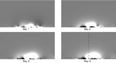
Figure 8: Images showing the locations of free magnetic energy storage in the x-z plane summed along the y-direction for the non-linear force free field. White denotes locations where there is excess free magnetic energy compared to that of a potential field. The image is set to saturate at $\pm 1\times 10^{27}$ ergs.

In Figure 8 the images illustrate the locations of free magnetic energy storage for days 1-4. The plots are in the x-z plane and give the free magnetic energy summed along the line of sight,

$$E(x,z)=A\int\frac{({\bf B}^{2}-{\bf B_{p}}^{2})}{8\pi}dy$$ (6)

where ${\bf{B}}$ is the magnetic field of the non-linear force-free field and ${\bf{B_{p}}}$ the magnetic field of the potential field satisfying the same normal field components on the boundaries. The factor $A$ represents the area of the column being summed over ($A=2.02\times 10^{16}$ cm²). The area factor is included so that the free energy along the line of sight is computed in units of ergs. In each plot the x-direction represents the full length of the computational box, but the z-direction is only half the height. White locations denote where the non-linear force-free field has a higher energy than the potential field when integrated along the line of sight (i.e locations where free magnetic energy is stored). Black denotes where the non-linear force-free field has a lower energy when integrated along the line of sight (i.e locations where there is no free energy). We note that while the non-linear force-free field must and does have a volume integrated energy that is greater than that of the potential field (see Figure 7), there is no restriction that in any sub-volume that this must always be true. Hence the negative values of the line integral quantity in Equation 6 are physically valid.

Figure 9: Graphs showing the free magnetic energy in units of $10^{27}$ ergs as a function of (a) $x$ at $z=0.12$ units and (b) $z$ at $x=3$ units along the dashed lines shown in Figure 8. Positive values denote locations where the non-linear force-free field energy has a higher energy compared to that of a potential field.

As the small scale convective motions advect the field between days 1 and 4, the locations of free magnetic energy storage expand up into the coronal volume and mainly lie in the center of the box. From these images it is clear that the main locations of free magnetic energy is low down in the corona (below $30$ Mm) and between the two main flux concentrations. It is built up at this location, as here the magnetic fields are the strongest and the energy injection through Poynting Flux the greatest. In addition, these field lines are the shortest and occupy a smaller volume.

While the images shown in Figure 8 are useful for illustrating the general spatial locations of free magnetic energy. Often such scaled images lead to misleading interpretation on the exact values. To quantify this, in Figure 9, graphs of the variation of free magnetic energy can be seen for day 4, along the paths given by the dashed lines in Figure 8. In Figure 9(a) the free magnetic energy can be seen as a function of x at a height of $7,300$ km ($z=0.12$ units). Positive values denote locations where the non-linear force-free field has a higher energy, negative values where it is lower (when integrated along the line of sight). From this graph it is clear that in the coronal volume the free energy is mainly positive. Near the center of the domain there is a small region where the non-linear force-free field has a lower energy than the potential field. However the negative value of the line of sight integrated free energy is small compared to the locations where it is positive. From this it can be seen that the scaling and color shown in Figure 8 exaggerates the level where the free magnetic energy is negative. In Figure 9(b) the variation of free magnetic energy can be seen as a function of $z$, taken at $x=3$ units. It is clear that along this cut the free energy is always positive. In general the amount of free energy available decreases with height in the box.

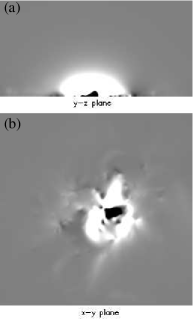
Figure 10: Images showing the locations of free magnetic energy storage on day 4 in (a) the $y-z$ plane summed along the $x$-direction and (b) the $x-y$ plane summed along the $z$-direction for the non-linear force free field. White denotes locations where there is excess free magnetic energy compared to that of a potential field. The same scaling is used as in Figure 8.

Alternative views of the free magnetic energy storage can be seen in Figure 10. In Figure 10(a) it is shown in the $y-z$ plane summed along the x-direction (Equation 7) and in Figure 10(b) for the $x-y$ plane summed along the z-direction (Equation 8). In each case results are shown for day 4 and the same scaling is used as in Figure 8.

$$E(y,z)=A\int\frac{({\bf B}^{2}-{\bf B_{p}}^{2})}{8\pi}dx$$ (7)

$$E(x,y)=A\int\frac{({\bf B}^{2}-{\bf B_{p}}^{2})}{8\pi}dz$$ (8)

Once again it is clear that the locations of free magnetic energy storage exist in the center of the computational box where the main flux concentrations are at their strongest. In Figure 10(b) the main spatial location where the line of sight integrated free energy is negative is surrounded by positive free energy locations. To determine why such a region exits, Figure 11 compares the photospheric magnetic field distribution of the active region to the location where the line of sight free magnetic energy is negative. In this plot thin solid lines denote positive flux, dashed lines negative flux and the thick solid line where the line of sight integrated free energy is $-6\times 10^{26}$ ergs or less. It can be clearly seen that the negative region is spatially correlated with the cancellation site between the positive and negative polarities. Therefore it is due to the removal of photospheric and coronal flux at this location as a result of flux cancellation (Figure 4).

4.3 Magnetic Helicity

As the coronal magnetic field is subjected to the small scale random motions, these motions not only inject magnetic energy into the field but also magnetic helicity (Démoulin & Pariat, 2009). This is seen by the increasing complexity of the field. To quantify this injection a calculation of relative magnetic helicity ($H_{r}$) is carried out. This quantity is defined as

$$H_{r}=\int_{v}{\bf{A.B}}d\tau-\int_{v}{\bf{A_{p}.B_{p}}}d\tau.$$ (9)

where $\bf A$ and $\bf B$ are the vector potential and magnetic field of the non-linear force-free field. Similarly $\bf A_{p}$ and $\bf B_{p}$ are the vector potential and magnetic field of a potential field which satisfies the same normal field components as that of the non-linear force-free field on all boundaries (namely $B_{z}$ on $z=0$ and $B_{n}=0$ on all other faces). The definition of relative magnetic helicity was first introduced by Berger & Field (1984) as an invariant and therefore meaningful measure of magnetic helicity. It should be noted that in constructing the potential field for the relative helicity calculation the technique described in Section 3.2 is used. The horizontal components of the vector potential on the base, $A_{xb}$ and $A_{yb}$, are identical for both the non-linear force-free and potential magnetic fields. This means that the expression for the relative helicity does not include an addition surface integral term.

In Figure 12 the graph shows the variation of the relative magnetic helicity as a function of time (solid line). From the behaviour of the curve it can be seen that over the first day there is no definite trend of helicity injection by the surface motions. The relative helicity oscillates between positive and negative values. In contrast, between days 1-4 there is a definite trend of positive helicity injection, with the relative helicity showing an increasing positive value. Positive helicity injection is consistent with observations that show that active regions in the southern hemisphere have a dominant positive helicity (Pevtsov et al., 1995). The dash-dot line in Figure 12 is a linear best fit to the relative helicity curve between days 1-4. The gradient of the line gives a helicity injection rate of $1.218\times 10^{34}$ Mx²s^-1. Such an increase of helicity within the coronal field can only be as the result of helicity injection through the lower boundary as a result of the relative motion of the magnetic fragments (Démoulin & Berger, 2003; Démoulin & Pariat, 2009) as during the period of observations there is no increase in magnetic flux. However, through considering the evolution of the magnetic elements in the magnetogram, there is no clear indication as to the origin of the helicity injection, as the dominant motion acting on the active region are small scale random motions.

Figure 11: Comparison of the underlying magnetic field distribution with locations were the non-linear force-free field has less energy than the potential field on day 4. In the plot positive and negative photospheric magnetic flux is given by the thin solid and dashed contours. The thick solid contour denotes the area where the non-linear force-free field has an energy less that $6\times 10^{26}$ergs of the corresponding potential field when summed in the z-direction.

In contrast, on comparing Figure 12 to the graphs of flux variation (Figure 4) and separation between the centers of flux elements (Figure 3), it can be seen that the positive helicity injection may possibly be related to large-scale properties of the evolution of the active region. To begin with on day 1 the flux peaks, after which it systematically starts to decrease. This decrease is the result of first convergence and then cancellation of the polarities along the internal PIL of the bipole. Secondly, around the same time the separation of the sources increases, so there is an overall divergence of the active region polarities. Either of these two processes (convergence/divergence) may result in the net positive helicity injection. However, within the present simulation we are unable to determine which. To compute this techniques such as Local Correlation Tracking would have to be applied (Chae, 2001; Pariat et al., 2005; Jeong & Chae, 2007). While there is no clear indication of its origin, a third possibility is that such a positive injection of helicity is consistent with the effect of differential rotation as will be discussed in Section 6.

While the relative helicity has a positive value the amount of helicity is small. Active regions containing fluxes of $1\times 10^{22}$Mx may well contain helicity on the order of $10^{42}-10^{44}$Mx² (Tian & Alexander, 2008). On studying the coronal field in more detail it is found that the random motions inject large amounts of both positive and negative helicity, but in near equal amounts over the four days of the simulation. This is what is expected from such motions, therefore resulting in a low net helicity.

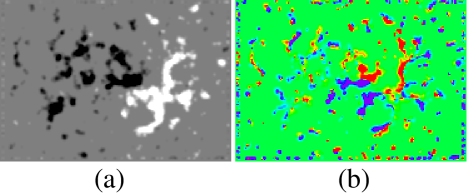
Figure 13: Comparison of (a) magnetic flux distribution and (b) distribution of the force-free parameter $\alpha$ on the base ($z=0$) at the end of day four. The magnetic field values are set to saturate at $\pm 100$G while the values of alpha saturate at $\pm 2.73\times 10^{-9}$ $m^{-1}$.

In Figure 13 a comparison of (a) the normal magnetic field component on the lower boundary and (b) the distribution of $\alpha$ on the lower boundary can be seen for the final time snapshot of the simulation. Similar plots were found at other times. In Figure 13(a) white/black represents positive/negative flux, while in Figure 13(b) red/blue denotes positive/negative values of $\alpha$. The magnetic field values are set to saturate at $\pm 100$G while the $\alpha$ values saturate at $\pm 2.73\times 10^{-9}$ m^-1. On comparing the distributions it can be seen that the spatial distribution of $\alpha$ is well correlated to that of the magnetic field. The distribution of $\alpha$ take two forms. First, in locations of strong field concentrations the $\alpha$ distribution takes the form of large coherent patterns. Secondly, it takes the form of small isolated patches of intermingled sign which lie in small flux concentrations. It is clear from comparing the two images, that within the large concentrations of flux, a single magnetic element of one polarity may contain both positive and negative values of $\alpha$. Such a mixture of positive and negative values of $\alpha$, as a result of small scale convective motions, support the results that the coronal field of the AR cannot be modeled by a linear force-free field as found in Section 2.2. The positive and negative $\alpha$ distributions are similar to the divided distribution of current used in the idealised model of Régnier (2009). An interesting feature of the comparison is that within the large flux concentrations the northern portions appear to contain more positive values of $\alpha$, while the southern portions have more negative values. In addition to the $\alpha$ values that lie within the center of the simulation, values may be seen along the edge of the magnetogram area. Such edge values are a pure boundary effect and should not be considered further.

Figure 12: Variation of relative magnetic helicity within the simulation as a function of time (solid line). The dash-dot line denotes a straight line fit to the positive trend seen between days 1-4. The gradient of the straight line gives an average helicity injection rate over days 1-4 of $1.218\times 10^{34}$ Mx²s^-1.

For the active region considered here no vector magnetogram data are available in order to compare observed $\alpha$ distributions or trends of $\alpha$ in the observations with those obtained within the simulation. In future with the launch of SDO and the SDO:HMI instrument, regular vector magnetic field data will be available which can be compared to future simulations applying this technique. Through this we will be able to determine how much helicity is injected due to small scale motions, and in addition how much must be injected by other effects (e.g. torsional Alfven waves). This provides a new tool for the quantification of such effects which may be applied directly to observations.

5 Simple Calculations

To determine if the rate of energy build-up within the present simulation is realistic, a simple order of magnitude calculation is carried out to determine the rate of inflow of energy into the lower boundary via the Poynting Vector, ${\bf S}=(c/4\pi){\bf E}\times{\bf B}$. The Poynting flux ($P$) through the lower boundary is,

$$P=-\frac{c}{4\pi}\int_{s}({\bf E}\times{\bf B}).{\bf{da}}$$ (10)

where ${\bf E}$ is the electric field and ${\bf{da}}=da{\hat{\bf n}}$. In order of magnitude terms this equation may be simplified to,

$$P\approx\frac{v_{h}B_{z}B_{h}A_{m}}{4\pi}$$ (11)

where $v_{h}$ is the typical horizontal velocity, $B_{z}$ a typical normal field component, $B_{h}$ a typical horizontal field strength and $A_{m}$ the area of energy input. The area of input is taken as the area of the observed magnetogram $A_{m}=4.7\times 10^{20}$ cm², $v_{h}=0.5kms^{-1}$ the peak flow rate of a supergranular cell. The values of the average field components are then taken to be $B_{z}=12$G and $B_{h}=2$G, where these values are determined from the initial potential field. Through this an upper estimate of the Poynting flux becomes $4.5\times 10^{25}$ ergs s^-1. This value is around a factor of 2 greater than the value deduced within the simulations of $2.5\times 10^{25}$ ergs s^-1. Although the order of magnitude calculation is larger by a factor of 2 this value is an over estimate as it assumes (i) the flow is always at the peak rate and (2) flows that are steady and systematic. In reality all elements in the magnetogram do not move at all times and in the simulations the flow is irregular. Taking this into account it can be seen that the simulation produces a realistic energy input into the coronal volume.

In the second calculation, we consider how important the energy input from the small convective motions is relative to an estimate of the radiative losses for the active region. The radiative losses in an optically thin plasma at coronal temperatures is given by,

$$E_{R}=n_{e}^{2}R(T)~{}~{}\mathrm{ergscm^{-3}s^{-1}}$$ (12)

where $n_{e}$ is the electron number density, $T$ the temperature and $R(T)$ the radiative loss function which is given by Rosner et al (1978) as,

$$R(T)\approx 10^{-17.73}T^{-2/3},~{}~{}\mathrm{6.3<log~{}T<7.0}$$ (13)

The average temperature of the active region is determined to be $log~{}T=6.41$ through using the SXT filter ratio technique on the Al.1 and AlMg filters. We take the volume of the coronal emitting plasma to be $10^{29}~{}$cm³. Note that this is not the volume of the computation box but rather an upper estimate of the volume of emitting plasma in the active region. Taking also an upper estimate of the electron number density to be $10^{9}$cm^-3, provides an upper estimate of the coronal radiative losses as $\sim 1\times 10^{25}$ ergs s^-1. This value can be seen to be of the same order as the energy build up due to the small scale convective motions.

While the two values are consistent with one-another, it should be noted that the free magnetic energy in the simulation is held within the coronal field and therefore not immediately accessible to heat the corona and account for the radiative losses. For such a process to take place an additional energy release mechanism, would have to act. Possible mechanisms include nanoflares (Parker, 1988; Browning et al., 2008; Wilmot-Smith et al., 2010) or turbulent reconnection(Heyvaerts & Priest, 1984). At this point it is unclear if such a mechanism may release the energy. Also the simple calculation does not take into account the effect of thermal conduction which is an important factor in the energy balance of hot coronal loops. However, taking these limitations into account, the calculation does show that convective motions may play a key role in the energy build up of the corona.

Using the rates of energy injection determined in the simulation and assuming that it remains constant over the life-time of the active region, it is possible to estimate how much free energy the active region could have on the 16th December, the start day of the present simulations, due to prior evolution as it rotated onto the disk and towards central meridian. Assuming that it emerged just before disk passage the active region would have evolved for 5 days. As a result the small scale convective motions would inject a total of $1.1\times 10^{31}$ergs of free magnetic energy into the coronal field. This value is 10$\%$ of the active region energy on the 16th December. While the energy may have been $10\%$ higher, we cannot use this to constrain the initial condition without having vector magnetic field data to constrain the distribution of $\alpha$ on the lower boundary.

6 Discussion and Conclusions

In this paper a new technique for modeling non-linear force-free fields directly from line of sight component magnetogram observations has been presented. The key new feature of this technique is that sequences of line of sight magnetograms can be directly used as lower boundary conditions to drive the evolution of coronal magnetic fields between successive force-free equilibria. As a result, the lower boundary condition in the model closely follows the observed magnetic field evolution as given by the observed line-of-sight magnetograms over the period of observations.

The technique is illustrated by applying it to MDI observations of a decaying active region, NOAA AR 8005. The active region was close to central meridian and in flux balance to a high degree. It was modeled over a 4 day period, where 61 individual SoHO:MDI 96 min magnetograms where available to use as lower boundary conditions. During this time the dispersal of the active region was mainly dominated by random motions due to small scale convective cells and flux cancellation along the internal polarity inversion line.

Through applying the 61 magnetograms as lower boundary conditions and simulating a continuous evolution of the surface and coronal field between them, the build up of free magnetic energy into the corona was studied. It should be noted here that the initial condition for the coronal field in the simulation was taken to be a potential field. Due to the availability of only line-of-sight component magnetograms this was the only unique choice. However at the time corresponding to the start of the simulation the actual coronal field of the active region need not have been potential. Therefore our aim was not to reproduce the evolution of the coronal loops as seen in coronal observations, but rather to study the trends of energy input over the period of four days, where this is deduced from using observed magnetograms.

When the initial coronal field is taken to be potential, the small-scale motions inject around $2.5\times 10^{25}$ ergs s^-1 of free magnetic energy, this energy is mainly stored in the low corona below 30 Mm. However, even if the initial state on the Sun was different, this would not significantly alter the trends of energy injection found within the simulation. To illustrate this we have repeated the simulation using an initial condition of a linear force-free field, with $\alpha$ values of $1.55\times 10^{-8}$m^-1 and $1.86\times 10^{-8}$m^-1. These values are 80$\%$ and 88$\%$ of the first resonant value of $\alpha$. Only positive values of $\alpha$ are chosen as the active region lies in the southern hemisphere. With these alternative initial conditions similar results and trends are found to those shown in Figure 7. The only difference is that the magnetic field has a higher initial energy. The subsequent rates of energy injection are $2.65\times 10^{25}$ ergs s^-1 and $2.8\times 10^{25}$ ergs s^-1 respectively. These values are consistent to those found when using the potential field. The slightly higher values occur due to the increased horizontal component of field in the linear-force free field leading to a higher Poynting flux. For all cases the energy injection through this new technique is consistent with estimates derived from poynting flux calculations. After just 4 days of evolution the free energy is 10$\%$ that of the potential field. Such energy buildup, is sufficient to explain the radiative losses at coronal temperatures within the active region ($1\times 10^{25}$ ergs s^-1). Therefore small scale convective motions play an integral part in the energy balance of the corona.

Through studying the evolution of the relative magnetic helicity in the coronal field, it was found that near equal amounts of positive and negative helicity are injected into the coronal field, but with a slight preference for positive helicity injection in the later stages. This is consistent with the active region being buffeted by small scale random motions and observations that show that active regions in the southern hemisphere have a preference for positive helicity (Pevtsov et al., 1995). One possible cause of this slight positive helicity injection is the effect of differential rotation. In the southern/northern hemisphere differential rotation will inject positive/negative helicity into the corona (DeVore, 2000). Démoulin et. al (2002) showed that helicity injection by differential rotation is composed of two terms, which for a decayed and dispersed active region are of opposite sign. The injection rate also increases with active region latitude and varies with active region tilt angle. During the short time period of our study, where the active region lies near the equator, we expect differential rotation to play only a minor role in ejecting positive helicity into the active region.

The new technique presented here has wide ranging applications for modeling the evolution of photospheric magnetic fields observed on the Sun and the subsequent effect these have on the coronal field over long periods of time. In future we shall use new high resolution, high cadence full disk vector magnetic field data from SDO:HMI in combination with coronal observations to constrain the initial condition. With this we may then compare the evolution of the coronal magnetic field with that seen in coronal observations. Under such constraints it will become a powerful tool to study the nature and properties of coronal magnetic fields.

DHM would like to thank UK STFC for their financial support and the Royal Society for funding a 81 processor supercomputer under their Research Grants Scheme. LMG would like to thank the Royal Society and Leverhulme Trust for financial support. We acknowledge the use of data provided by the SoHO/MDI instrument. The authors would like to thank the referee for his constructive comments which have improved this paper.

References

- Archontis et al. (2004) Archontis, V., Moreno-Insertis, F., Galsgaard, K., Hood, A., & O’Shea, E. 2004, A&A, 426, 1047
- Benz (2008) Benz, A. O. 2008, Living Reviews in Solar Physics, 5, 1
- Berger & Field (1984) Berger, M. A., & Field, G. B. 1984, Journal of Fluid Mechanics, 147, 133
- Bobra et al. (2008) Bobra, M. G., van Ballegooijen, A. A., & DeLuca, E. E. 2008, ApJ, 672, 1209
- Browning et al. (2008) Browning, P. K., Gerrard, C., Hood, A. W., Kevis, R., & van der Linden, R. A. M. 2008, A&A, 485, 837
- Chae (2001) Chae, J. 2001, ApJ, 560, L95
- Charbonneau (2005) Charbonneau, P. 2005, Living Reviews in Solar Physics, 2, 2
- Cremades et al. (2006) Cremades, H., Bothmer, V., & Tripathi, D. 2006, Advances in Space Research, 38, 461
- Démoulin et. al (2002) Démoulin, P., Mandrini, C. H., van Driel-Gesztelyi, L., López Fuentes, M. C. & Aulanier, G. 2002, Sol. Phys., 207, 87
- Démoulin & Berger (2003) Démoulin, P., & Berger, M. A. 2003, Sol. Phys., 215, 203
- Démoulin & Pariat (2009) Démoulin, P., & Pariat, E. 2009, Advances in Space Research, 43, 1013
- De Rosa et al. (2009) De Rosa, M. L., et al. 2009, ApJ, 696, 1780
- DeVore (2000) DeVore, C. R. 2000, ApJ, 539, 944
- Fan (2009) Fan, Y. 2009, ApJ, 697, 1529
- Galsgaard et al. (2007) Galsgaard, K., Archontis, V., Moreno-Insertis, F., & Hood, A. W. 2007, ApJ, 666, 516
- Green & Kliem (2009) Green, L. M., & Kliem, B. 2009, ApJ, 700, L87
- Heyvaerts & Priest (1984) Heyvaerts, J., & Priest, E. R. 1984, A&A, 137, 63
- Jeong & Chae (2007) Jeong, H., & Chae, J. 2007, ApJ, 671, 1022
- Jing et al. (2010) Jing, J., Tan, C., Yuan, Y., Wang, B., Wiegelmann, T., Xu, Y., & Wang, H. 2010, ApJ, 713, 440
- Leighton (1964) Leighton, R. B. 1964, ApJ, 140, 1547
- Mackay et al. (2000) Mackay, D. H., Gaizauskas, V., & van Ballegooijen, A. A. 2000, ApJ, 544, 1122
- Mackay & Gaizauskas (2003) Mackay, D. H., & Gaizauskas, V. 2003, Sol. Phys., 216, 121
- Mackay & van Ballegooijen (2005) Mackay, D. H., & van Ballegooijen, A. A. 2005, ApJ, 621, L77
- Mackay & van Ballegooijen (2006a) Mackay, D. H., & van Ballegooijen, A. A. 2006, ApJ, 641, 577
- Mackay & van Ballegooijen (2006b) Mackay, D. H., & van Ballegooijen, A. A. 2006, ApJ, 642, 1193
- Mackay & van Ballegooijen (2009) Mackay, D. H., & van Ballegooijen, A. A. 2009, Sol. Phys., 260, 321
- Magara (2004) Magara, T. 2004, ApJ, 605, 480
- Metcalf et al. (2008) Metcalf, T. R., et al.2008, Sol. Phys., 247, 269
- Murray & Hood (2008) Murray, M. J., & Hood, A. W. 2008, A&A, 479, 567
- Parker (1988) Parker, E. N. 1988, ApJ, 330, 474
- Pariat et al. (2005) Pariat, E., Démoulin, P., & Berger, M. A. 2005, A&A, 439, 1191
- Pevtsov et al. (1995) Pevtsov, A. A., Canfield, R. C., & Metcalf, T. R. 1995, ApJ, 440, L109
- Priest (1982) Priest, E. R. 1982, Dordrecht, Holland ; Boston : D. Reidel Pub. Co. ; Hingham,, 74P
- Regnier & Priest (2007) Regnier, S., & Priest, E. R. 2007, ApJ, 669, L53
- Régnier (2009) Régnier, S. 2009, A&A, 497, L17
- Savcheva & van Ballegooijen (2009) Savcheva, A., & van Ballegooijen, A. 2009, ApJ, 703, 1766
- Scherrer et al. (1995) Scherrer, P.H., Bogart, R.S., Bush, R.I., Hoeksema, J.T., Kosovichev, A.G., Schou, J., Rosenburg, W., Springer, L., Tarbell, T.D., et al.: 1995, Sol. Phys., 162, 129
- Schrijver et al. (2006) Schrijver, C. J., et al. 2006, Sol. Phys., 235, 161
- Su et al. (2009a) Su, J. T., Sakurai, T., Suematsu, Y., Hagino, M., & Liu, Y. 2009, ApJ, 697, L103
- Su et al. (2009b) Su, Y., van Ballegooijen, A., Lites, B.W., DeLuca, E.E., Golub, L., Grigis, P.C., Huang, G., & Ji, H. 2009, ApJ, 691, 105
- Tian & Alexander (2008) Tian, L., & Alexander, D. 2008, ApJ, 673, 532
- van Ballegooijen et al. (2000) van Ballegooijen, A. A., Priest, E. R., & Mackay, D. H. 2000, ApJ, 539, 983
- van Ballegooijen (2004) van Ballegooijen, A. A. 2004, ApJ, 612, 519
- Wheatland & Régnier (2009) Wheatland, M. S., & Régnier, S. 2009, ApJ, 700, L88
- Wilmot-Smith et al. (2010) Wilmot-Smith, A. L., Pontin, D. I., & Hornig, G. 2010, A&A, 516, A5
- Woltjer (1958) Woltjer, L. 1958, Proceedings of the National Academy of Science, 44, 489
- Yeates et al. (2007) Yeates, A. R., Mackay, D. H., & van Ballegooijen, A. A. 2007, Sol. Phys., 245, 87
- Yeates et al. (2008) Yeates, A. R., Mackay, D. H., & van Ballegooijen, A. A. 2008, Sol. Phys., 247, 103
- Yeates & Mackay (2009) Yeates, A. R., & Mackay, D. H. 2009, ApJ, 699, 1024
- Yeates et al. (2010) Yeates, A. R., Attrill, G. D. R., Nandy, D., Mackay, D. H., Martens, P. C. H., & van Ballegooijen, A. A. 2010, ApJ, 709, 1238
- Yeates et al. (2010) Yeates, A. R. Mackay, D. H. van Ballegooijen, A.A., 2010, J. Geophys. Res., accepted