Gluon Propagators in Linear Covariant Gauge

Abstract:

The implementation of the linear covariant gauge on the lattice faces a conceptual problem: using the standard compact discretization, the gluon field is bounded, while the four-divergence of the gluon field satisfies a Gaussian distribution, i.e. it is unbounded. This can give rise to convergence problems when a numerical implementation is attempted. In order to overcome this problem, one can use different discretizations for the gluon field or consider an SU($N_{c}$) group with sufficiently large $N_{c}$. One can also consider small values of the gauge parameter $\xi$ and study numerically the limiting case of $\xi\to 0$, i.e. the Landau gauge. These different approaches will be discussed here.

1 Why study the linear covariant gauge?

Extensive numerical simulations on very large lattices [1, 2, 3, 4, 5, 6, 7] have shown that, in three and in four space-time dimensions, the Landau gluon propagator displays a massive solution at small momenta and the Landau ghost propagator is essentially free in the same limit. (For a recent review and various comments, see respectively [8] and [9].) These results are not in agreement with the original Gribov-Zwanziger confinement scenario [10, 11] but they can be explained in the so-called refined Gribov-Zwanziger framework [12, 13].

A natural extension of these works in Landau gauge would be to consider the linear covariant gauge, which has the Landau gauge as a limiting case. However, until recently, the numerical gauge fixing for the linear covariant gauge [14, 15, 16] was not satisfactory. In Reference [17] we introduced a new implementation of the linear covariant gauge on the lattice that solves most problems encountered in earlier implementations. The final goal is to evaluate Green’s functions numerically in the linear covariant gauge and, in particular, in the Feynman gauge. This could allow a nonperturbative evaluation of the gauge-invariant off-shell Green’s functions of the pinch technique [18, 19].

2 The Linear Covariant Gauge on the Lattice

In the continuum, the linear covariant gauge is obtained by imposing the gauge condition

$$\partial_{\mu}A^{b}_{\mu}(x)=\Lambda^{b}(x)\;,$$ (1)

where the real-valued functions $\Lambda^{b}(x)$ are generated using a Gaussian distribution

$$\exp{\left\{\,-\frac{1}{2\xi}\int d^{d}x\sum_{b}\left[\Lambda^{b}(x)\right]^{2}\,\right\}}$$ (2)

with width $\sqrt{\xi}$. The limiting case $\xi\to 0$, which implies $\Lambda^{b}(x)=0$, yields the Landau gauge.

On the lattice, one can fix the Landau gauge by minimizing the functional

$${\cal E}_{LG}[U^{g}]=-\mbox{Tr}\sum_{\mu,x}g(x)U_{\mu}(x)g^{\dagger}(x+e_{\mu})$$ (3)

with respect to the gauge transformations $\{g(x)\}$. Here, $U_{\mu}(x)$ are (fixed) link variables and $g(x)$ are site variables, both belonging to the SU($N_{c}$) group. The sum is taken over all lattice sites $x$ and directions $\mu$, and Tr indicates trace in color space. By considering a one-parameter subgroup

$$g(x,\tau)\,=\,\exp\left[i\tau\gamma^{b}(x)\lambda^{b}\right]$$ (4)

of the gauge transformation $\{g(x)\}$, one can verify that the stationarity condition for the functional ${\cal E}_{LG}[U^{g}]$ implies the (lattice) gauge condition

$$\sum_{\mu}\,A_{\mu}^{b}(x)\,-\,A_{\mu}^{b}(x-e_{\mu})\,=\,0\;,$$ (5)

where

$$A_{\mu}(x)\,=\,(\,2i\,)^{-1}\,\left[U_{\mu}(x)-U_{\mu}^{\dagger}(x)\right]_{traceless}$$ (6)

is the usual lattice discretization for the gluon field. Also, from the second variation of ${\cal E}_{LG}[U^{g}]$ one can obtain a discretized version of the Faddeev-Popov operator

$${\cal M}^{ab}\,=\,-D_{\mu}^{ab}\,\partial_{\mu}\;,$$ (7)

where $\,D_{\mu}^{ab}\,$ is the covariant derivative. Clearly, for the gauge-fixed configurations, i.e. for all local minima of the functional ${\cal E}_{LG}[U^{g}]$, this operator is positive-definite. This set of local minima defines the first Gribov region $\Omega$ [10, 11].

In Reference [17] we have introduced the minimizing functional

$${\cal E}_{LCG}[U^{g},g,\Lambda]\;=\;{\cal E}_{LG}[U^{g}]\,+\,\Re\;Tr\sum_{x}\,i\,g(x)\,\Lambda(x)\;,$$ (8)

which is a natural extension of the Landau functional (3). Here $\Re$ indicates real part. One should stress that, in the numerical minimization, the link variables $U_{\mu}(x)$ are gauge-transformed to $g(x)U_{\mu}(x)g^{\dagger}(x+e_{\mu})$, while the $\Lambda^{b}(x)$ functions do not get modified. It is easy to verify, using again a one-parameter subgroup $g(x,\tau)$, that this functional leads to the lattice linear covariant gauge condition

$$\sum_{\mu}\,A^{b}_{\mu}(x)\,-\,A^{b}_{\mu}(x-e_{\mu})\,=\,\Lambda^{b}(x)\;.$$ (9)

Note that the above relation and periodic boundary conditions yield

$$\sum_{x}\Lambda^{b}(x)\,=\,0\;.$$ (10)

This equality must be enforced numerically, within machine precision, when the functions $\Lambda^{b}(x)$ are generated using the Gaussian distribution (2). Also note that the second variation (with respect to the parameter $\tau$) of the term $\,i\,g(x)\,\Lambda(x)\,$ is purely imaginary and it does not contribute to the Faddeev-Popov matrix ${\cal M}$. Clearly, having a minimizing functional for the linear covariant gauge implies that the set of its local minima defines the first Gribov region $\Omega$ and that the corresponding Faddeev-Popov operator ${\cal M}$ is positive-definite. This should allow the extension of the Gribov-Zwanziger approach to the linear covariant gauge. In particular, one should be able to study the region $\Omega$ for the case of a gauge parameter $\xi\neq 0$ and to compare the results with the analytic study carried out in Reference [20] for small values of $\xi$.

In order to relate the lattice approach to the continuum, one should note [16] that the continuum relation (1) can be made dimensionless by multiplying both sides by $a^{2}g_{0}$. Since in $d$ dimensions and in the SU($N_{c}$) case one has $\beta=2N_{c}/(a^{4-d}g_{0}^{2})$, it is clear that the lattice quantity

$$\frac{\beta/(2N_{c})}{2\xi}\sum_{x,b}\left[a^{2}g_{0}\Lambda^{b}(x)\right]^{2}\,=\,\frac{1}{2\sigma^{2}}\sum_{x,b}\left[a^{2}g_{0}\Lambda^{b}(x)\right]^{2}\,=\,\frac{1}{2\sigma^{2}}\sum_{x,b}\left[\Lambda_{latt}^{b}(x)\right]^{2}$$ (11)

gives

$$\frac{1}{2\xi}\frac{1}{a^{4-d}g_{0}^{2}}\int\frac{d^{d}x}{a^{d}}\sum_{b}\left[a^{2}g_{0}\Lambda^{b}(x)\right]^{2}\;=\;\frac{1}{2\xi}\int d^{d}x\sum_{b}\left[\Lambda^{b}(x)\right]^{2}$$ (12)

in the formal continuum limit. Thus, the continuum gauge parameter $\xi$ corresponds to a width

$$\sigma\,=\,\sqrt{\frac{2N_{c}\xi}{\beta}}$$ (13)

for the Gaussian distribution on the lattice and only for $\beta=2N_{c}$ does one have $\sigma=\sqrt{\xi}$.

3 Numerical Simulations

The functional ${\cal E}_{LCG}[U^{g},g,\Lambda]$ — see Eqs. (3) and (8) — is linear in the gauge transformations $\{g(x)\}$. Thus, the gauge-fixing algorithms usually employed in the Landau case [21, 22, 23] can be used also for the linear covariant gauge and, in principle, the numerical gauge fixing should not be a problem for this gauge. Nevertheless, as explained in the Abstract, any formulation of the linear covariant gauge on the lattice faces a conceptual problem. Indeed, the gluon field $A^{a}_{\mu}(x)$, usually defined as in Equation (6), is bounded while the functions $\Lambda^{b}(x)$ satisfy a Gaussian distribution [see Equation (2)] and are thus unbounded. Then, it is clear that Eq. (9) cannot be satisfied if $\Lambda^{b}(x)$ is too large [24]. As a consequence, one has to deal with convergence problems when numerically imposing the linear covariant gauge condition. Also, these problems become more severe as the width $\sqrt{\xi}$ of the Gaussian distribution becomes larger and/or as the lattice volume becomes larger. On the lattice, as shown above, the width $\sigma$ of the Gaussian distribution is given by $\sigma=\sqrt{2N_{c}\xi/\beta}$. Thus, these convergence problems are more severe also for small values of the coupling $\beta$. In particular, for $\beta<2N_{c}$ the lattice width $\sigma$ is larger than the continuum width $\sqrt{\xi}$.

In References [17, 25] we have presented tests of convergence of the numerical gauge fixing in the SU(2) case for relatively small lattice volumes, $\beta=4$ and values of $\xi$ up to 0.5. [Recall that for $\beta=4$ one has $\sigma=\sqrt{\xi}$ in the SU(2) case.] We have also checked that the quantity $D_{L}(p^{2})p^{2}$, where $D_{L}(p^{2})$ is the longitudinal gluon propagator, is approximately constant for all cases considered, as predicted by Slavnov-Taylor identities. This verification failed in previous formulations of the lattice linear covariant gauge [15, 16].

In order to overcome the convergence problems discussed above and be able to simulate at lattice coupling $\beta$ smaller than $4$ in the SU(2) case, we considered different discretizations of the gluon field. In particular, we used the angle (or logarithmic) projection [26] and the stereographic projection [27] (for a slightly different implementation of the stereographic projection see also [28]). Note that, in the latter case, the gluon field is unbounded even for a finite lattice spacing $a$. Our results [17, 25] clearly show that the angle projection is already an improvement compared to the standard discretization and that the best convergence is obtained when using the stereographic projection. In References [17, 25] we also presented preliminary results for the transverse gluon propagator using the stereographic projection. From these results one clearly sees that, as in Landau gauge, the transverse propagator is more infrared suppressed when the lattice volume increases. At the same time, for a fixed volume $V$, this propagator is also more infrared suppressed when the gauge parameter $\xi$ increases. The latter result is in agreement with Reference [15]. One should, however, stress that the stereographic projection cannot be extended to SU($N_{c}$) groups with $N_{c}>2$. Thus, in the SU(3) case one should probably rely on the logarithmic projection.

Finally, one should note that, in the SU(2) case, the value $\sigma=\sqrt{\xi}$, i.e. $\beta=4$, corresponds to a lattice spacing $a\approx 0.001$ fm. On the contrary, in the SU(3) case, one has $\sigma=\sqrt{\xi}$ for $\beta=6$, corresponding to $a=0.102$ fm. Also, for a fixed t’Hooft coupling $g_{0}^{2}N_{c}$, we have $\beta\propto N_{c}^{2}$ and $\sigma\propto\sqrt{1/N_{c}}$. This suggests that simulations for the linear covariant gauge are easier in the SU($N_{c}$) case for large $N_{c}$. In Reference [29] we tested this hypothesis by simulating the SU(2), SU(3) and SU(4) cases for a gauge parameter $\xi=1$ and lattice volumes up to $V=32^{4}$ for several values of the coupling $\beta$. We find that the convergence problems are indeed reduced when the number of colors $N_{c}$ is larger.

4 The Limit $\xi\to 0$

In the continuum, the Landau gauge condition is defined by considering the usual Faddeev-Popov Lagrangian for the linear covariant gauge and by taking the limit $\xi\to 0$. On the contrary, on the lattice, this gauge has been studied without considering this limit, but by imposing directly the gauge condition

$$\partial_{\mu}\,A_{\mu}^{b}(x)\,=\,0\,,$$ (14)

which is usually called the Lorenz gauge. The latter gauge condition is fixed numerically by minimizing the functional (3). Using our implementation of the linear covariant gauge, it seems natural to study the Landau gauge by numerically considering the limit $\xi\to 0$, in analogy with the definition in the continuum. One should also note that, in this limit, the width of the Gaussian distribution (2) goes to zero and, therefore, the convergence problems discussed above should be reduced — or eliminated — even for large lattice volumes and for $\beta$ values in the scaling region. Moreover, since in the limit $\xi\to 0$ the Gaussian distribution becomes a Dirac delta function $\delta(\Lambda)$, this limit can be studied numerically by using different approximations of the delta function.

Here we consider three possible sequences of functions, labelled by a parameter $\alpha$, leading to a delta function in the limit $\alpha\to 0$, i.e.

1. the Gaussian distribution

   $$f_{G}(\Lambda)\,=\,\frac{e^{-\Lambda^{2}/(2\alpha_{G}^{2})}}{\sqrt{2\pi\alpha_{G}^{2}}}\,,$$ (15)

2. the Triangle distribution

   $$f_{T}(\Lambda)\,=\,\left\{\begin{array}[]{l l}\frac{(1-\Lambda/\alpha_{T})}{\alpha_{T}}&\quad\mbox{for}\,\Lambda\in[0,\alpha_{T}]\\[5.69054pt] \frac{(1+\Lambda/\alpha_{T})}{\alpha_{T}}&\quad\mbox{for}\,\Lambda\in[-\alpha_{T},0]\\[5.69054pt] 0&\quad\mbox{for}\,\Lambda\notin[-\alpha_{T},\alpha_{T}]\\ \end{array}\right.$$ (16)

3. and the Rectangular distribution

   $$f_{R}(\Lambda)\,=\,\left\{\begin{array}[]{l l}\frac{1}{\alpha_{R}}&\quad\mbox{for}\,\Lambda\in[-\alpha_{R}/2,\alpha_{R}/2]\\[5.69054pt] 0&\quad\mbox{for}\,\Lambda\notin[-\alpha_{R}/2,\alpha_{R}/2]\\ \end{array}\right.\,.$$ (17)

Note that the last two distributions are bounded. Also note that the average value of $\Lambda^{2}$ using these three distributions is respectively given by $\alpha_{G}^{2}$, $\alpha_{T}^{2}/6$ and $\alpha_{R}^{2}/12$. Thus, by setting

$$\alpha_{G}\,=\,\frac{\alpha_{T}}{\sqrt{6}}\,=\,\frac{\alpha_{R}}{\sqrt{12}}$$ (18)

we have three different distributions with the same moment of inertia.

We have done exploratory tests considering, in the SU(2) case, the lattice volume $V=32^{4}$ at $\beta=2.2$. For the gauge-fixing parameters $\alpha$ we used the values $\alpha_{G}\approx 0.144338,0.0288674$ and $0.00288674$ for the Gaussian distribution, $\alpha_{T}\approx 0.353553,0.0707107$ and $0.00707107$ for the triangle distribution and $\alpha_{R}=0.5,0.1$ and $0.01$ for the rectangular distribution. Note that these values satisfy the relations in Eq. (18). Also, the values of $\alpha_{G}$ correspond to the continuum values $\xi\approx 0.0114584,4.5833\,10^{-4}$ and $4.5833\,10^{-6}$, respectively. For comparison, we have also done simulations directly at $\xi=0$, i.e. imposing the Lorenz condition (14). Results for the longitudinal $D_{L}(p^{2})$ and the transverse $D_{T}(p^{2})$ gluon propagators are shown in Figs. 1–4. One sees that the limit $\alpha\to 0$ is smoothly approached in the gluon sector and that the results are independent of the considered distribution. In particular, it is clear in Figs. 1–2 that the theoretical prediction $D_{L}(p^{2})=\sigma^{2}/p^{2}$, with $\sigma^{2}=\alpha_{G}^{2}=\alpha_{R}^{2}/12$, is satisfied by the data obtained with these three distributions. At the same, a value of $\sigma^{2}=\alpha_{G}^{2}\approx 0.144338^{2}\approx 0.02$ (see Fig. 4), which corresponds to the continuum value $\xi\approx 0.01$, already seems to give results in quantitative agreement with the Landau case.

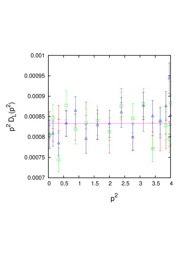
Figure 1: Plot of $p^{2}D_{L}(p^{2})$ as a function of $p^{2}$ (in lattice units) for $\alpha_{R}=0.1$ ($+$), $\alpha_{T}\approx 0.0707107$ ($\square$) and $\alpha_{G}\approx 0.0288674$ ($\triangle$). We also show the theoretical value $\sigma^{2}=\alpha_{R}^{2}/12\approx 0.0008333$.

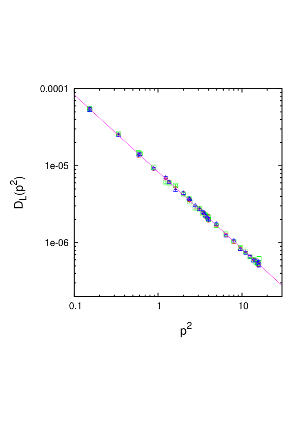
Figure 2: Plot of $D_{L}(p^{2})$ as a function of $p^{2}$ (both in lattice units), using the logarithmic scale in both axes, for $\alpha_{R}=0.01$ ($+$), $\alpha_{T}\approx 0.00707107$ ($\square$) and $\alpha_{G}\approx 0.00288674$ ($\triangle$). We also show the theoretical prediction $\alpha_{R}^{2}/(12p^{2})$.

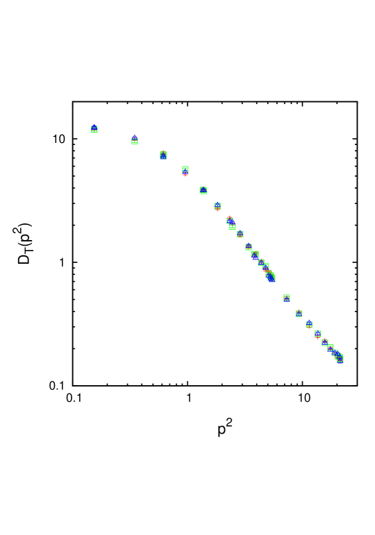
Figure 3: Plot of $D_{T}(p^{2})$ as a function of $p^{2}$ (both in lattice units), using the logarithmic scale in both axes, for $\alpha_{R}=0.1$ ($+$), $\alpha_{T}\approx 0.0707107$ ($\square$) and $\alpha_{G}\approx 0.0288674$ ($\triangle$).

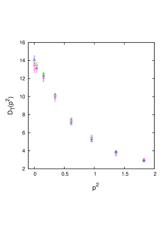
Figure 4: Plot of $D_{T}(p^{2})$ as a function of $p^{2}$ (both in lattice units) for $\alpha_{G}\approx 0.144338$ ($+$), $\alpha_{G}\approx 0.0288674$ ($\square$), $\alpha_{G}\approx 0.00288674$ ($\triangle$) and $\alpha_{G}=0$ ($\times$).

5 Conclusions

We have found a minimizing functional for the linear covariant gauge that is a simple generalization of the Landau-gauge functional. This approach solves most problems encountered in earlier implementations. Simulations for large lattice volumes, $\beta$ values in the scaling region and a large gauge parameter $\xi$ can probably be done with SU(3) and SU(4) using the logarithmic projection, allowing a non-perturbative study of Green’s functions. Finally, the approach to the limiting case $\xi\to 0$, i.e. the Landau gauge, can also be studied numerically. Here we have investigated this limit considering three different distributions defining the gauge condition.

References

- [1] I. L. Bogolubsky, E. M. Ilgenfritz, M. Muller-Preussker and A. Sternbeck, The Landau gauge gluon and ghost propagators in 4D SU(3) gluodynamics in large lattice volumes, PoS LAT2007 (2007) 290.
- [2] A. Cucchieri and T. Mendes, What’s up with IR gluon and ghost propagators in Landau gauge? A puzzling answer from huge lattices, PoS LAT2007 (2007) 297.
- [3] A. Sternbeck, L. von Smekal, D. B. Leinweber and A. G. Williams, Comparing SU(2) to SU(3) gluodynamics on large lattices PoS LAT2007 (2007) 340.
- [4] A. Cucchieri and T. Mendes, Constraints on the IR behavior of the gluon propagator in Yang-Mills theories, Phys. Rev. Lett. 100 (2008) 241601.
- [5] A. Cucchieri and T. Mendes, Constraints on the IR behavior of the ghost propagator in Yang-Mills theories, Phys. Rev. D 78 (2008) 094503.
- [6] I. L. Bogolubsky, E. M. Ilgenfritz, M. Muller-Preussker and A. Sternbeck, Lattice gluodynamics computation of Landau gauge Green’s functions in the deep infrared, Phys. Lett. B 676 (2009) 69.
- [7] M. Gong, Y. Chen, G. Meng and C. Liu, Lattice Gluon Propagator in the Landau Gauge: A Study Using Anisotropic Lattices, Mod. Phys. Lett. A 24 (2009) 1925.
- [8] A. Cucchieri, and T. Mendes, Numerical test of the Gribov-Zwanziger scenario in Landau gauge, PoS QCD-TNT09 (2009) 026.
- [9] A. Cucchieri, T. Mendes, The Saga of Landau-Gauge Propagators: Gathering New Ammo, [arXiv:1101.4779 [hep-lat]].
- [10] V. N. Gribov, Quantization of non-Abelian gauge theories, Nucl. Phys. B 139 (1978) 1.
- [11] D. Zwanziger, Fundamental modular region, Boltzmann factor and area law in lattice gauge theory, Nucl. Phys. B 412 (1994) 657.
- [12] D. Dudal, J. A. Gracey, S. P. Sorella, N. Vandersickel and H. Verschelde, A Refinement of the Gribov-Zwanziger approach in the Landau gauge: Infrared propagators in harmony with the lattice results, Phys. Rev. D 78 (2008) 065047.
- [13] S. P. Sorella, D. Dudal, M. S. Guimaraes and N. Vandersickel, Features of the Refined Gribov-Zwanziger theory: propagators, BRST soft symmetry breaking and glueball masses, [arXiv:1102.0574 [hep-th]].
- [14] L. Giusti, Nucl. Phys. B 498, 331 (1997).
- [15] L. Giusti, M. L. Paciello, S. Petrarca, C. Rebbi and B. Taglienti, Results on the gluon propagator in lattice covariant gauges, Nucl. Phys. Proc. Suppl. 94 (2001) 805.
- [16] A. Cucchieri, A. Maas and T. Mendes, Linear Covariant Gauges on the Lattice, Comput. Phys. Commun. 180 (2009) 215.
- [17] A. Cucchieri, T. Mendes and E. M. S. Santos, Covariant gauge on the lattice: a new implementation, Phys. Rev. Lett. 103 (2009) 141602.
- [18] D. Binosi and J. Papavassiliou, Pinch Technique: Theory and Applications, Phys. Rept. 479 (2009) 1.
- [19] J. M. Cornwall, Open issues in confinement, for the lattice and for center vortices, PoS QCD-TNT09 (2009) 007.
- [20] R. F. Sobreiro and S. P. Sorella, A study of the Gribov copies in linear covariant gauges in Euclidean Yang-Mills theories, JHEP 0506 (2005) 054.
- [21] A. Cucchieri and T. Mendes, Critical slowing down in SU(2) Landau gauge fixing algorithms, Nucl. Phys. B471 (1996) 263.
- [22] A. Cucchieri and T. Mendes, Study of critical slowing down in SU(2) Landau gauge fixing, Nucl. Phys. Proc. Suppl. 53 (1997) 811.
- [23] A. Cucchieri and T. Mendes, Critical slowing-down in SU(2) Landau-gauge-fixing algorithms at beta infinity, Comput. Phys. Commun. 154 (2003) 1.
- [24] J. Rank, Thermal Screening Masses in the Standard Model of Strong and Electroweak Interactions, Ph.D. thesis, Bielefeld University, January 1998 (file available at http://www.physik.uni-bielefeld.de/ theory/e6/publiframe.html).
- [25] A. Cucchieri, T. Mendes and E. M. S. Santos, Simulating linear covariant gauges on the lattice: a new approach, PoS QCD-TNT09 (2009) 009.
- [26] K. Amemiya and H. Suganuma, Effective mass generation of off-diagonal gluons as the origin of infrared Abelian dominance in the maximally Abelian gauge in QCD, Phys. Rev. D 60 (1999) 114509.
- [27] L. von Smekal, D. Mehta, A. Sternbeck and A. G. Williams, Modified Lattice Landau Gauge, PoS LAT2007 (2007) 382.
- [28] F. Gutbrod, Gauge singularities in the SU(2) vacuum on the lattice, Nucl. Phys. B720 (2005) 116.
- [29] A. Cucchieri, T. Mendes, G. M. Nakamura and E. M. S. Santos, Feynman gauge on the lattice: new results and perspectives, [arXiv:1101.5080 [hep-lat]].