On the Initial Conditions for Star Formation and the IMF

Abstract

Density probability distribution functions (PDFs) for turbulent self-gravitating clouds should be convolutions of the local log-normal PDF, which depends on the local average density $\rho_{\rm ave}$ and Mach number ${\cal M}$, and the probability distribution functions for $\rho_{\rm ave}$ and ${\cal M}$, which depend on the overall cloud structure. When self-gravity drives a cloud to increased central density, the total PDF develops an extended tail. If there is a critical density or column density for star formation, then the fraction of the local mass exceeding this threshold becomes higher near the cloud center. These elements of cloud structure should be in place before significant star formation begins. Then the efficiency is high so that bound clusters form rapidly, and the stellar initial mass function (IMF) has an imprint in the gas before destructive radiation from young stars can erase it. The IMF could arise from a power-law distribution of mass for cloud structure. These structures should form stars down to the thermal Jeans mass $M_{J}$ at each density in excess of a threshold. The high-density tail of the PDF, combined with additional fragmentation in each star-forming core, extends the IMF into the Brown Dwarf regime. The core fragmentation process is distinct from the cloud structuring process and introduces an independent core fragmentation mass function (CFMF). The CFMF would show up primarily below the IMF peak.

1 Introduction

The density probability distribution function for supersonically turbulent gas is a log-normal when self-gravity is not important (Vázquez-Semadeni, 1994; Passot & Vázquez-Semadeni, 1998; Padoan, Nordlund & Jones, 1997; Lemaster & Stone, 2008; Federrath et al., 2010; Price, 2011). A power law extension at high density appears with self-gravity (Klessen, 2000; Vázquez-Semadeni et al, 2008; Kritsuk, Norman & Wagner, 2010). Observations of column density show extended PDFs in star-forming regions and nearly pure log-normal PDFs in non-star-forming regions, which is consistent with these theoretical trends (Kainulainen et al., 2009; Froebrich & Rowles, 2010; Lombardi, Lada & Alves, 2010).

Here we consider a log-normal PDF that applies locally for the local average density and Mach number in a cloud. The PDF for the whole cloud is the convolution of this with the probability distribution function for these quantities, which vary with position when gravity and energy dissipation are important. The result has a power-law tail if the Mach number is constant, and a gradually falling tail if the Mach number decreases with increasing average density.

The convolution-PDF depends on the ratio of maximum to minimum average cloud density, i.e., the core-to-edge average density ratio in a GMC. The PDF also depends on cloud mass because the maximum Mach number does. As a cloud evolves from a diffuse state to a strongly self-gravitating state, the density PDF develops an extended tail where the star formation rate and the efficiency per unit free fall time become high.

The convolution-PDF is a useful starting point for approximations of internal cloud structure. We use it to determine several interesting characteristics of star formation: the cumulative mass as a function of density, the fraction of the local mass in the form of high-density cores, and the efficiency of star formation per unit free fall time, all as functions of average density or cloud radius. The first of these derived quantities illustrates why the gas consumption time for most tracers is longer than the dynamical time. The second and third are important for understanding why bound clusters form.

Cloud structure may also be relevant to the stellar initial mass function (IMF; see review in Shadmehri & Elmegreen, 2011). Pre-stellar gas cores share many properties with protostars and young stars, including the mass distribution function in the power-law regime (e.g., Motte, André &, Neri, 1998; Rathborne et al., 2009), the autocorrelated positions of each (Johnstone et al., 2000, 2001; Enoch et al., 2006; Young et al., 2006; Schmeja, Kumar, & Ferreira, 2008), and the mass fractions compared to the whole cloud. Here we consider the IMF model by Padoan & Nordlund (2002) with some modifications to determine IMFs in clouds with convolution-PDFs.

Cloud structure characterized approximately by a convolution-PDF could be in place before significant star formation begins. This would help explain observations of short formation times and high cluster efficiencies, even when the efficiency per unit free fall time is small on average (Krumholz & Tan, 2007). It might also explain the persistence of a near-universal IMF in the presence of intense stellar feedback. While some radiative heating may be important to limit the overproduction of Brown Dwarfs (Bate, 2009), intense radiation from massive stars can prevent the formation or collapse of low-mass cores, giving a top-heavy IMF (Krumholz et al., 2010) unlike that usually observed in regions of massive star formation.

In what follows, we present convolution-PDFs and derived quantities for various ratios of center-to-edge average cloud densities and Mach numbers (Sect. 2). Applications to the IMF are discussed in Section 3.

2 Convolution PDFs

The density PDF in a region of the interstellar medium depends on the distribution of local Mach number ${\cal M}$ and local average density, $\rho_{ave}$, and may be written

$$P_{\rm PDF}(\rho)=\int_{\rho_{\rm ave\;min}}^{\rho_{\rm ave\;max}}P_{\rm PDF,local}(\rho|\rho_{\rm ave})P_{\rm ave}(\rho_{\rm ave})d\rho_{\rm ave}.$$ (1)

$P_{\rm PDF,local}(\rho|\rho_{\rm ave})$ is the conditional probability distribution function for density $\rho$, given the average $\rho_{\rm ave}$. We use the usual log-normal relation for this PDF, assuming it comes from supersonic turbulence:

$$P_{\rm PDF,local}=(2\pi D^{2})^{-1/2}e^{-0.5\left(\ln(\rho/\rho_{\rm pk})/D\right)^{2}}$$ (2)

per unit $\ln(\rho)$. The density $\rho_{\rm pk}$ is at the peak of the local PDF and the log-normal width is $D$. The peak and average densities are related by

$$\rho_{\rm pk}=\rho_{\rm ave}e^{-0.5D^{2}},$$ (3)

and the Mach number and log-normal width are related approximately by (Padoan, Nordlund & Jones, 1997)

$$D^{2}=\ln(1+0.25{\cal M}^{2}).$$ (4)

The probability distribution function for the average density, $P_{\rm ave}(\rho_{\rm ave})$, and the relation between Mach number and density, depend on the history of the cloud. A cloud that has just formed from some gas collection process or a cloud that is gravitationally unbound will be somewhat uniform in average density, while a cloud that has contracted gravitationally or is collapsing will be centrally condensed. To cover this range of conditions, we assume that the average density varies with radius in a spherical cloud as

$$\rho_{\rm ave}(r)=\rho_{\rm edge}{{r_{\rm edge}^{\alpha}+r_{\rm core}^{\alpha}}\over{r^{\alpha}+r_{\rm core}^{\alpha}}}$$ (5)

where the degree of central condensation depends on the ratio

$${\cal C}={{\rho_{\rm ave}(r=0)}\over{\rho_{\rm edge}}}.$$ (6)

The core radius, $r_{\rm core}$, is used to avoid a density singularity and to control the maximum density contrast in the average cloud. The probability distribution function for $\rho_{\rm ave}$ is given by the relative volumes of different densities,

$$P(\rho_{\rm ave})=4\pi r^{2}\left(d\rho_{\rm ave}/dr\right)^{-1}.$$ (7)

After normalization and the definition $z=\rho_{\rm edge}/\rho_{\rm ave}(r)$, with $r_{\rm core}/r_{\rm edge}=\left({\cal C}-1\right)^{-1/\alpha}$, we get

$$P(\rho_{\rm ave})d\rho_{\rm ave}={{3{\cal C}\left(z{\cal C}-1\right)^{(3-\alpha)/\alpha}}\over{\alpha\left({\cal C}-1\right)^{3/\alpha}}}dz.$$ (8)

The resultant PDF for all density is then, from equation (1)

$$P_{\rm PDF,total}(y)={{3{\cal C}}\over{\alpha(2\pi)^{0.5}}}\int_{1/{\cal C}}^{1}\exp\left(-{{\ln^{2}(yze^{0.5D^{2}})}\over{2D^{2}}}\right){{\left(z{\cal C}-1\right)^{(3-\alpha)/\alpha}}\over{D\left({\cal C}-1\right)^{3/\alpha}}}dz,$$ (9)

per unit $\ln y$, where we have normalized the local density to the average cloud edge density, $y=\rho/\rho_{\rm edge}$. Note that $y$ is the local normalized density, including turbulent fluctuations, while $z$ is the inverse of the average density, not including the turbulent fluctuations, both normalized to the edge density. The width $D$ of the log-normal generally varies with position $r$, and so $D$ can be a function of $z$.

For large $yz$, the exponent becomes small and the fluctuations infrequent. Thus the integral is dominated by $z<1/y$ at large $y$, and for constant $D$, scales with only the density distribution for average density, which means $P_{\rm PDF,total}\propto y^{-3/\alpha}$. This is the power law part of the density PDF at large density relative to the cloud edge (Kritsuk, Norman & Wagner, 2010).

Figure 1 shows the total density PDF in the lower left panel for three ratios of the core-to-edge average density contrast, ${\cal C}$, in the case of constant Mach number equal to 5 (i.e., constant $D=1.41$) and radial-density slope $\alpha=1.5$. These are the three solid-line curves in the figure. The dashed red curve is a pure log-normal PDF with the same constant $D$. The abscissa is the normalized local density, not the average, and so is not a simple function of radius. In fact, each local density $\rho$ corresponds to a wide range of possible radii depending on the local compressions (i.e., on the local log-normal PDFs). The figure indicates that the PDF develops a power-law tail as ${\cal C}$ increases. The slope of this power-law is indicated by the straight line segment, which has a slope of $-3/\alpha=-2$. For larger ${\cal C}$, the length of the power law segment increases.

Figure 1 also shows a case with variable Mach number ${\cal M}$ as a dotted blue line. We consider here a cloud with virialized sub-condensations, in which case the local Mach number scales with $\left(M[r]/r\right)^{1/2}$. This is normalized to some Mach number at the cloud edge, ${\cal M}_{\rm edge}$:

$${\cal M}(r)={\cal M}_{\rm edge}\left(M[r]r_{\rm edge}/M_{\rm total}r\right)^{1/2}.$$ (10)

The radial mass variation is from $M(r)=\int_{0}^{r}4\pi r^{2}\rho_{\rm ave}(r)dr$. For an approximately uniform column density, equation (10) gives the Larson (1981) size-linewidth law. We consider a minimum ${\cal M}=1$ to get density fluctuations from turbulence. Thus ${\cal M}$ is taken to be the larger of 1 and the value given by equation (10). When ${\cal M}$ varies in this way, it gets smaller for higher average density and closer to the cloud center. Then the log-normal Kernel of the convolution-PDF gets narrower with increasing $\rho_{\rm ave}$, and the total PDF curves down below a power-law tail. The power law tail occurs when the Mach number is constant throughout a cloud. This situation may not be realistic for a cloud more than several crossing times old, and if a constant ${\cal M}$ is observed, it may indicate extreme cloud youth.

The upper left panel of Figure 1 shows the cumulative mass fractions for the same cases as in the bottom left panel. These are the mass fractions for relative densities greater than the values on the abscissa. They were determined by integrating over all radii for each relative local density, $y$, i.e., using equation 9,

$$f_{\rm Mass}(>y)={{\int_{y}^{y_{\rm max}}P_{\rm PDF,total}(y)dy}\over{\int_{0}^{y_{\rm max}}P_{\rm PDF,total}(y)dy}}.$$ (11)

Note that $P_{\rm PDF,total}$ is defined as per unit $\ln(y)$, so in fact we integrated over $yd\ln(y)$ for equal intervals of $d\ln(y)$, but this is the same as $dy$ written above. We assumed $y_{\rm max}=10^{6}$ for computational reasons. Figure 1 indicates that the mass fraction of dense gas at high density is several orders of magnitude larger for a power-law tail than for a log-normal PDF with the same Mach number. This means that with a threshold density for star formation, the star formation rate should be much larger in clouds that are centrally condensed (${\cal C}>>1$) than in uniform clouds (${\cal C}=1$). This is in agreement with observations (e.g., Lada, Lombardi & Alves, 2009, 2010) and recent simulations (Cho & Kim, 2011).

The bottom right panel of Figure 1 shows the fraction of the mass at a density larger than the threshold density, versus the normalized average density. The top right panel shows the same quantity as a function of normalized radius. This mass fraction of threshold gas is not uniform throughout a cloud but increases as the average density increases. If stars form in threshold gas, then they have a greater probability per unit gas mass of forming near the center for ${\cal C}>>1$. This threshold gas fraction is also related to the efficiency of star formation measured as a star-to-total mass ratio. A high threshold gas fraction favors the formation of bound clusters.

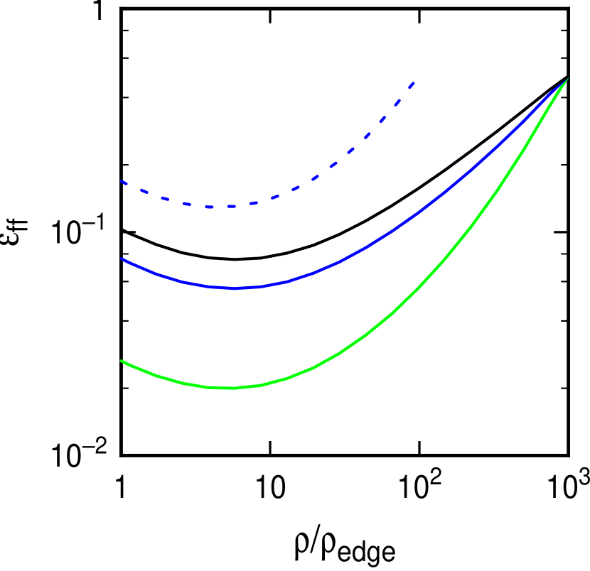
Figure 2: The local efficiency of star formation per unit free fall time is plotted as a function of the local normalized density $y=\rho/\rho_{\rm edge}$, from equation (13). The cloud concentration is ${\cal C}=10^{2}$, $10^{3}$, and $10^{4}$ for green, blue, and black curves, and the threshold density is $y_{\rm thres}=10^{3}$ with constant $D$. The dotted blue curve has variable $D$ with ${\cal C}=10^{3}$ and $y_{\rm thres}=10^{2}$.

Figure 2 shows the local efficiency of star formation per unit dynamical time, $\epsilon_{\rm dyn}$, versus the normalized local density. The local efficiency is the fraction of the gas mass that turns into stars in a local dynamical time, measured in some part of the cloud where the density might be higher than average. This concept is useful if stars form at a characteristic threshold density, $\rho_{\rm thres}$, and evolution toward this density occurs at a rate proportional to the local dynamical rate, $(G\rho)^{1/2}$. As the local average density around a star-forming clump increases toward the center of the clump, the fraction of the local mass at or above this density that is also above the threshold density increases, because the lower density gas that does not participate in star formation gets left behind. This means $\epsilon(\rho)$ increases with $\rho$. Numerical simulations use variable $\epsilon(\rho)$ also: if the threshold for star formation in a simulation is taken to be a low density, then the efficiency for star formation defined at that density has to be low too, to get the overall rate correct (e.g., Teyssier et al., 2010). If we consider a clumpy cloud with contours at density $\rho$, then the average star formation rate per unit volume inside these contours may be written

$${\rm SFR}=\epsilon_{\rm dyn}(\rho)(G\rho)^{1/2}\int_{\rho}^{\infty}\rho P_{\rm PDF,tot}(\ln\rho)d\ln\rho.$$ (12)

The integral is the mass at densities larger than $\rho$ inside the contours where $\epsilon_{\rm dyn}(\rho)$ is measured; it also appears in equation (11). Inside these contours we can envision higher and higher densities until we reach the threshold density, whereupon a fixed high fraction of the gas gets into stars. We take this fixed fraction to be 0.5, in which case

$$\epsilon_{\rm dyn}(\rho)=0.5\left({{\rho_{\rm thres}}\over{\rho}}\right)^{1/2}\left({{f_{\rm Mass}[\rho_{\rm thres}]}\over{f_{\rm Mass}[\rho]}}\right).$$ (13)

This is the quantity shown in Figure 2 using the convolution PDF. A similar diagram for a log-normal PDF was shown in Elmegreen (2008), where $\epsilon_{\rm dyn}(\rho)$ was considered in more detail.

The importance of this result, and of the density dependence for total efficiency (Fig. 1 - right hand side), is that they allow us to understand the formation of bound clusters in only a few dynamical times, even though the average efficiency per unit free fall time is observed to be low, like a few percent (e.g. Krumholz & Tan, 2007). The point is that a cloud does not have to wait for a time equal to the dynamical time multiplied by the inverse of this average low efficiency in order to build up a sufficiently high total efficiency to make a bound cluster. This would require $\sim 20$ dynamical times for the average density, which is too long compared to observations (Elmegreen, 2007). In fact, the efficiency per unit free fall time and the total efficiency are high near the cloud center from the beginning of the star formation process because most of the gas at $\rho_{\rm thres}$ is initially clustered there.

3 Applications to the IMF

The density PDF may also have some relevance to the stellar IMF. Padoan & Nordlund (2002) considered the IMF to result from a power law function of core mass $M$ multiplied by the probability that $M$ exceeds the thermal Jeans mass $M_{\rm J}$. This probability equals the integral over the distribution function of Jeans mass, from $M_{\rm J}=0$ to $M_{\rm J}=M$. The distribution function for Jeans mass was related to the density PDF in a one-to-one fashion using the relation between $M_{\rm J}$ and density. For the density PDF, Padoan & Nordlund (2002) assumed a log-normal. The extension of this log-normal into a power law PDF at high density in the present paper affects their IMF at low mass because the high density part contributes to the low $M_{J}$ values and to the probability that $M>M_{J}$ at low $M_{J}$.

We follow this IMF model with some modifications. First, the mass function for cloud structure in the supersonic regime is taken to be a power law with a slope $\alpha$ dependent on the slope $\beta$ of the density power spectrum, which for long lines of sight through a cloud, is the same as the slope of the column density power spectrum. This dependency is $\alpha\approx 4.35-0.71\beta$ (Shadmehri & Elmegreen, 2011), and for commonly observed $\beta=-2.8$, is $\alpha=2.35$, the Salpeter function slope. Thus the mass function for stars is related to the mass function for cloud structure in the supersonic regime, as in Padoan & Nordlund (2002).

These mass functions come primarily from the size distribution function for substructure, which is a power law in turbulent media when the power spectrum is a power law. Each mass equals approximately the structure’s volume multiplied by the boundary density used to define that structure (Shadmehri & Elmegreen, 2011). As a result, the mass function for cloud structure in the supersonic regime is nearly independent of the density PDF. This model contrasts with that of Hennebelle & Chabrier (2008), who assume that the IMF comes directly from an integral over the PDF of log-density, with stellar mass mapping out the Jeans mass so that low density regions form high mass stars. In the present model, all stars throughout the power-law portion of the IMF form at all densities above a threshold.

Second, gas forms stars only in regions that have a mass exceeding the local thermal Jeans mass, regardless of the shape of these regions. Elongated or irregular structures tend to collapse first into more irregular shapes (the eccentricity of an ellipsoidal shape increases during collapse – Hunter, 1962; Fujimoto, 1968), and then gradually into globules or cores that are collection points for gas draining down filaments. The condition for strong self-gravity means that the substructures defined by a certain density threshold, having a mass larger than the thermal Jeans mass at that density, have a high probability of turning into stars.

A third condition for star formation concerns the magnetic field. Magnetic diffusion is not essential for star formation because the gas can always move parallel to the field until the mass-to-flux ratio in the collecting core exceeds the critical value for collapse (e.g., Li et al., 2010). However, if the field energy density is large compared to the gravitational energy density, then this motion has to be over a long distance and that takes a lot of time. Turbulent media mix gas on crossing time scales, so only processes that are either fast or persistent can occur to completion. As a result, stars tend to form where the field diffuses out rapidly.

This diffusion constraint means that star formation occurs in regions that are shielded from background near-uv starlight by more than a few magnitudes of visible-wavelength extinction. H₂ accumulation takes only $\sim 1$ magnitude of visual extinction (Spitzer & Jenkins, 1975), which is not enough to prevent the ionization of elements heavier than Helium. CO accumulation takes another magnitude or so of visible extinction, depending on density. Neither condition alone is enough to cause the magnetic diffusion rate to drop to within a factor of 10 of the dynamical rate. Thus molecular cloud envelopes and diffuse molecular cloud tails in cometary structures (e.g., the rho Ophiuchus and Orion molecular clouds have long cometary tails), should have long magnetic diffusion times, long lifetimes, and relatively little star formation (Elmegreen, 2007). This is the essential reason why the consumption time of CO in the galaxy is much longer than the star formation time in each OB association. After self-gravity or external pressures compress part of a cloud, the extinction to the center can exceed several magnitudes. Then the ionization fraction drops to a new equilibrium regulated by cosmic rays. Magnetic diffusion becomes rapid in this case. As a result, rapid star formation requires a threshold cloud column density of $\sim 4$ magnitudes of visual extinction in all directions to background starlight (8 mag. through the cloud: McKee, 1989; Johnstone, Di Francesco & Kirk, 2004; Heiderman et al., 2010; Lada, Lombardi & Alves, 2009, 2010), primarily to get the magnetic field out of the contracting gas.

There could be a threshold density for star formation as well as a threshold column density. The distinction between the two may be hard to determine for solar neighborhood-type clouds. A threshold density might arise when the scaling of ionization fraction with density changes from $n^{-1/2}$ to n^-1 or faster as a result of changes in the dominant recombining species (Elmegreen 1978). It could also arise when atoms and molecules deplete onto grains faster than the dynamical time, removing key components of the gas-phase ion chemistry, or when tiny grains grow or get destroyed without reformation, removing an important component of the total ion collision cross section that normally resists magnetic diffusion (Elmegreen 2007). All of these processes speed up magnetic diffusion and they all seem to operate at a density between $10^{5}$ cm^-3 and $10^{6}$ cm^-3 for the solar neighborhood. Thus we consider this a threshold density, $\rho_{\rm thres}$, where the magnetic diffusion rate relative to the dynamical rate begins to change significantly. Threshold densities have been observed by Lada, Evans & Falgarone (1997); Gao & Solomon (2004); Wu et al. (2005); Evans (2008); Wu et al. (2010); Lada, Lombardi & Alves (2009, 2010) and others.

The column density constraint for thermal and radiative shielding, which gets the ionization fraction into the cosmic-ray dominated regime, and the density threshold for a suddenly heightened magnetic diffusion rate, introduce a third component to the theory of star formation and the IMF discussed in this paper. Although these are physically and geometrically different conditions, we represent them as one condition here and simply require the density to exceed a threshold for our cloud models. In giant molecular clouds, the column density exceeds the shielding threshold on average before the local density exceeds the threshold for rapid diffusion. Then the local density threshold is most relevant for star formation. In other regions where the density is high and the column density is not, such as supernova shells, the condition for star formation is the opposite at first (i.e., before shell gravitational instabilities and local collapse).

A fourth component of the IMF is the fragmentation of cloud structures during the final stages, when the gas collapses, stars compete for mass, disks form, interact and shed tidal debris, stars and Brown Dwarfs get ejected from dense cores, and so on, all shown in numerical simulations. Fragmentation during and after collapse involves different physical processes than turbulent fragmentation on GMC scales. Turbulent fragmentation produces power law mass functions (even with log-normal density PDFs), but collapse fragmentation can produce something else. This core fragmentation mass function (CFMF) should be an important component of the IMF, but it is rarely discussed and it has not been measured systematically for star-forming regions. Elmegreen (2000) considered a CFMF that is uniform in $\log M$ and suggested that the IMF below the thermal Jeans mass reflects this CFMF exclusively. Swift & Williams (2008) also noted that core fragmentation can broaden the IMF, while Goodwin et al. (2008) showed that core fragmentation into multiple stars can give a better IMF than a one-to-one correspondence between core mass and final stellar mass. Shadmehri & Elmegreen (2011) discuss the CFMF in detail.

We find in the cloud models that without a CFMF, the IMF cannot extend into the Brown Dwarf regime for realistic cloud Mach numbers and realistic variations of these Mach numbers with position or average density in a cloud. This is unlike the situation in Padoan & Nordlund (2002), who proposed very high and constant Mach numbers to reach a thermal Jeans mass in the Brown Dwarf regime. For constant temperature, the density has to be higher than average by a factor of $100$ to make the thermal Jeans mass smaller than average by a factor of 10. This seems necessary if there is no CFMF to broaden the stellar mass range in the cores. Getting that far into the tail of a log-normal density PDF without having the PDF drop too much is difficult. The log-normal PDF has a count of volume elements at density $\rho$ per unit log-density that is $\exp\left(-0.5\left[\ln\left\{\rho/\rho_{\rm pk}\right\}/D\right]^{2}\right)$ where $\rho_{\rm pk}$ is the density at the peak of the log-normal and $D$ is the dispersion. The average density in this PDF is $\rho_{\rm ave}=\rho_{\rm pk}\exp\left(0.5D^{2}\right)$. This means that the maximum value the PDF can have at a density of $100\rho_{\rm ave}$ occurs for a dispersion where $\left(\ln\left[100\right]+0.5D^{2}\right)/D$ is a minimum. This minimum is at $D=3.035$ and equals the same value, 3.035. For $D^{2}=\ln\left(1+0.25{\cal M}^{2}\right)$ (Padoan, Nordlund & Jones, 1997), the Mach number has to be ${\cal M}=200$ in this case, which is too high, and the PDF is down from the peak by $\exp\left(-0.5\times 3.035^{2}\right)=0.01$, which is too low. Alternatively, we could ask what is the ratio of the density PDF at $\rho=100\rho_{\rm ave}$ compared to the density PDF at $\rho=\rho_{\rm ave}$? This ratio should be large to have a relatively large number of Brown Dwarfs in the Padoan & Nordlund (2002) model. It has a maximum of unity at infinite $D$, so we ask what is the ratio at some reasonable $D$, such as that for Mach number ${\cal M}<100$, which gives $D<2.79$. There, the ratio is 2.6%, which is also too small. Thus, a theory of the IMF based on a log-normal density PDF alone, or even an extension of the log-normal with a power-law to modestly high density (see below), does not give enough high density material to make a significant number of Brown Dwarfs if their mass is close to the local thermal Jeans mass. We need either a density pdf in the supersonic regime that extends to extremely high density as a power law or other slowly varying function, or sub-fragmentation inside each Jeans mass. Brown Dwarf formation at extreme densities in collapse models was found by Bonnell, Clark, & Bate (2008). Sub-fragmentation can give a range of stellar or brown dwarf masses that extends downward for a much larger factor than what the dispersion in the density PDF can give alone. This is what we mean by a core fragment mass function. It is different than a single-valued efficiency of star formation in each core, which does not help to extend the low-mass stellar range relative to the IMF peak mass. Only a broad function of efficiencies, which is the CFMF in our model, can do this.

The shape of the CFMF is not known, but if we consider that cloud structures denser than $\rho_{\rm thres}$ fragment via turbulence into a power law mass distribution, and that only structures more massive than the thermal Jeans mass for the local density have the opportunity to form stars, then the CFMF is the part of the final IMF below the average thermal Jeans mass. This means that the shape of the CFMF is the shape of the IMF below the peak around $0.3\;M_{\odot}$. Note that the CFMF can be the same for all cloud structures and the summed IMF from them will still have the power law mass function of the cloud structure above the peak (Elmegreen, 2000). The CFMF is visible on the scale of clusters and OB associations only for masses below the peak. However, in very young clusters where the substructures from turbulent fragmentation are still visible as subclusters of protostars, the CFMF may be observed directly as the relative mass distribution function for these protostars inside each subcluster. If the CFMF is universal, then the protostellar mass function inside each subcluster, scaled to the subcluster mass, should be the same for all subcluster masses. Here is where competitive accretion and other local processes involving relative mass should dominate the IMF.

These hypotheses for star formation and the IMF may be summarized as follows: (1) stars form in cloud structures that are hidden from outside radiation by $>4$ mag of visual extinction in all directions, (2) they form fastest where the density $\rho$ exceeds a threshold value, $\rho>\rho_{\rm thres}\sim 10^{5}m_{\rm H2}$ cm^-3, (3) they form in cloud structures that have a $dN/dM\propto M^{-\alpha}$ mass function ($\alpha\sim 2$ to 2.5, the Salpeter function) for all densities above the threshold and for a wide range of masses, (4) they form only in those structures that have masses exceeding the local thermal Jeans mass, and (5) they form by fragmentation in these structures, with a universal core fragmentation mass function (CFMF). The density PDF enters the IMF through the distribution function of Jeans mass (Padoan & Nordlund, 2002), which is the distribution function of the lower mass limit to the power law for each density exceeding $\rho_{\rm thres}$.

Whether individual stars form by competitive accretion, using mass from all over a cloud (Bonnell & Bate, 2006), or by monolithic collapse (Shu, 1977; McKee & Tan, 2002) using mass from a pre-existing core, would seem to depend on evolutionary stage. Early on, when filaments are still draining onto cores, each core and all of its stars effectively accrete from relatively far away using gas from the filament and beyond. Later on, when dense cores may become displaced from their filaments or the filaments become empty, the core evolution is more monolithic. In addition, for any evolutionary stage, the most centrally condensed cores will produce the most monolithic-like collapse, i.e., without severe sub-fragmentation (Peters et al., 2010). Still, central condensation is also a result of age: rapid accretion for young cores adds turbulent energy and mixes the core material, preventing strong central condensations from starting. All of these processes should happen over a range of time and spatial scales during star formation, so both competitive accretion in loose sub-clusters and monolithic collapse inside centrally concentrated cores should happen simultaneously in a large cloud complex.

With this model, the total IMF that results from star formation in a cloud is the integral of the turbulent fragmentation power law over all the cloud parts denser than $\rho_{\rm thres}$, with lower limits to each turbulent fragmentation mass equal to the thermal Jeans mass at the local density. We write this as

$$P_{\rm IMF}\left(M_{\rm star}\right)=\int_{\rho_{\rm thres}}^{\infty}M_{\rm gas}^{-2.35}H\left[M_{\rm gas}-M_{\rm J}\left(\rho\right)\right]P_{\rm PDF,total}\left(\ln\rho\right)d\rho,$$ (14)

where, P_PDF,total is the probability distribution function for density in the whole cloud, measured per unit $\ln(\rho)$. The mass integral includes a density multiplied by this probability, $\rho P_{\rm PDF,total}d\ln\rho$, and $\rho d\ln\rho$ is replaced by $d\rho$. The other terms are as follows: $P_{\rm IMF}$ is the IMF, i.e., the probability distribution function of forming a star or Brown Dwarf with a mass between $M_{\rm star}$ and $M_{\rm star}+dM_{\rm star}$; $H$ is the Heaviside Function, equal to 0 for negative argument and 1 for positive argument, and $M_{\rm J}\left(\rho\right)$ is the thermal Jeans mass, which is a function of local density, $\propto\rho^{-1/2}$, assuming a constant thermal temperature for the present paper.

The stellar mass on the left of equation (14), $M_{\rm star}$, is related to the mass of a gas fragment in the integral, $M_{\rm gas}$, by the CFMF probability distribution function, $P_{\rm CFMF}(f)df$ for $f=M_{\rm star}/M_{\rm gas}$. We could therefore evaluate equation (14) by substituting $M_{\rm star}/f$ for $M_{\rm gas}$ in the integral, multiplying the result by $P_{\rm CFMF}(f)$, and integrating over $f$ from 0 to 1. When $M_{\rm star}<M_{\rm J}$, the Heaviside function of $(M_{\rm star}/f-M_{\rm J})$ cuts the integration limits for $f$ to 0 and $M_{\rm star}/M_{\rm J}$, making the IMF depend on the shape of $P_{\rm CFMF}(f)$. When $M_{\rm star}>M_{\rm J}$ the integration limits for $f$ are 0 to 1 and the integral over $f$ is independent of $M_{\rm star}$, leaving the IMF with the $M_{\rm star}^{-2.35}$ dependence from the clumps. Other analytical expressions involving the CFMF are in Elmegreen (2000) and Shadmehri & Elmegreen (2011).

To evaluate the IMF numerically, we consider that the relative proportion of the incidents of $f$ is $P_{\rm CFMF}(f)$, so the distribution of $M_{\rm star}$ for each $M_{\rm gas}$ comes from the equation

$${{\int_{M_{\rm min}/M_{\rm gas}}^{M_{\rm star}/M_{\rm gas}}P_{\rm CFMF}(f)df}\over{\int_{M_{\rm min}/M_{\rm gas}}^{1}P_{\rm CFMF}(f)df}}=X,$$ (15)

where X is a number uniformly distributed between 0 at $M_{\rm star}=M_{\rm min}$ and 1 at $M_{\rm star}=M_{\rm gas}$ ($X$ can be a random number or a sequence of regularly spaced numbers in this interval). In the lower limit of the integral, $M_{\rm min}$ is taken equal to $0.01$. To evaluate the IMF, we determine $P_{\rm PDF,total}(y)$ as discussed above, normalize $M_{\rm J}$ to unity at $y=y_{\rm thres}$, and choose $P_{\rm CFMF}(f)=1/f$ to make the IMF flat below $M_{J}$.

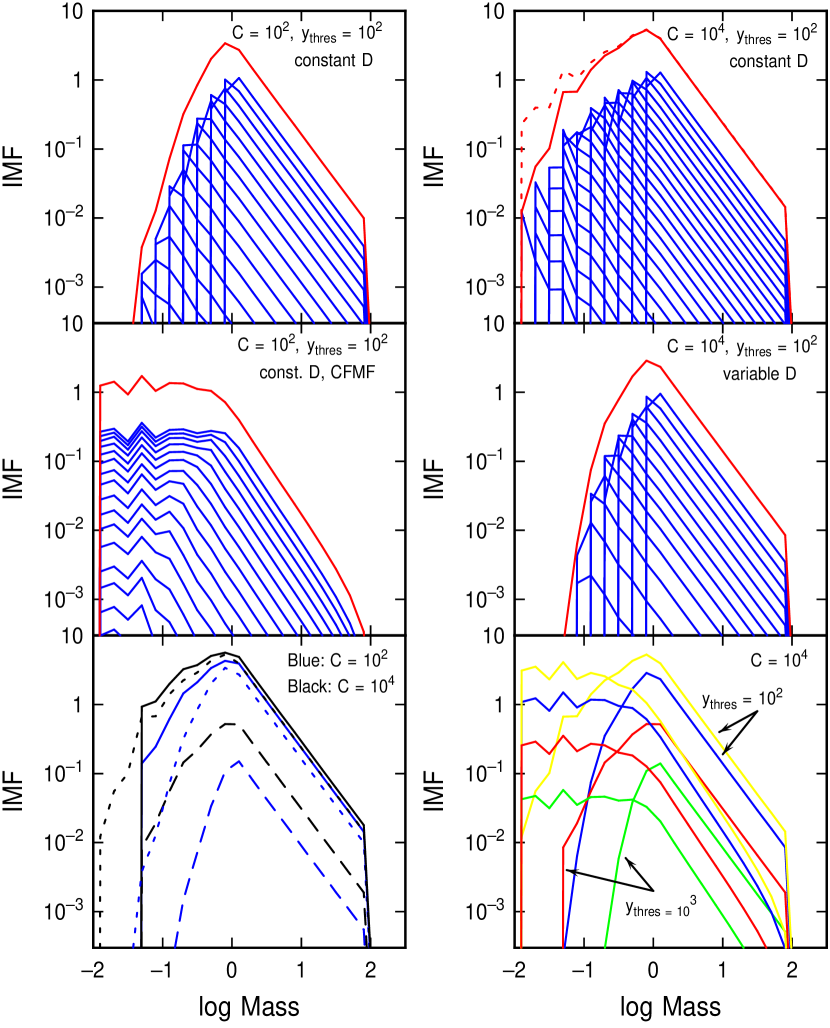
Figure 3: Stellar IMFs for a model with a Salpeter slope for cloud cores more massive than the local thermal Jeans mass, and either a direct correspondence between stellar and core masses (peaked curves) or a core fragmentation mass function that has a uniform probability for the star/core mass fraction per unit log $M$ (curves with a flat part at low $M$). Other assumptions in the IMF are a threshold density $y_{\rm thres}$ and no star formation in cores less massive than the Jeans mass. Red curves in the top four panels are summed IMFs for the whole cloud, and blue curves are components of this IMF for different relative local densities $y$. ${\cal C}$ is the cloud concentration parameter and $D$ is the dispersion in the log-normal part of the convolution-PDF. In the lower left, solid-line curves have a constant Mach number ${\cal M}=20$ and $y_{\rm thres}=10^{3}$; dotted curves have constant ${\cal M}=5$ and $y_{\rm thres}=10^{2}$; dashed curves have constant ${\cal M}=5$ and $y_{\rm thres}=10^{3}$. In the lower right, ${\cal C}=10^{4}$ for all cases; yellow curves have $y_{\rm thres}=10^{2}$ and constant Mach number ${\cal M}=5$; blue curves have $y_{\rm thres}=10^{2}$ and variable Mach number with edge value ${\cal M}_{\rm edge}=5$; red curves have $y_{\rm thres}=10^{3}$ and ${\cal M}=5$, while green curves have $y_{\rm thres}=10^{3}$ and variable Mach number with ${\cal M}_{\rm edge}=5$. Each color in the lower right has one curve with no CFMF and another curve with a CFMF.

Figure 3 shows sample IMFs generated from equations (14) and (15). In the top four panels, the summed IMF for the whole cloud is shown as a solid red curve (at the top of all the other curves), and the IMFs for each relevant $y$ value, with logarithmic spacings of $y$, are shown as blue curves (recall $y$ measures the local density, including turbulent compression: $y=\rho/\rho_{\rm edge}$). A relevant $y$ value is one that exceeds the threshold density for star formation. In the top two panels and middle-right panel, there is no clump fragmentation mass function ($P_{\rm CFMF}(f)=$ a delta function, i.e., $f$ is constant). In the middle-left panel, there is a CFMF, $P_{\rm CFMF}(f)=$constant in equal intervals of $\ln f$. When there is no CFMF, each blue curve consists of a power law at masses larger than the Jeans mass for that $y$ value, and a sudden drop at lower mass. This illustrates our assumption that stars form only with masses above the local Jeans mass, with no spread from a fragmentation mass function in these cases. Also in these three panels, increasing $y$ corresponds to a decreasing local Jeans mass, and therefore a decreasing peak mass in the blue curve. When there is a CFMF, in the middle-left panel, each blue curve for separate $y$ again has a power-law decrease above the local Jeans mass, but now there is a spread in stellar mass below the local Jeans mass from the CFMF. Because we assumed in this case $P_{\rm CFMF}(f)=$constant in equal intervals of $\ln f$, the IMF below each local Jeans mass is also constant for equal intervals of $\log M_{\rm star}$, i.e., the blue curves are flat.

The summed IMF in each of these four cases has the same general shape as the local IMFs. When there is no CFMF, the summed IMF has a power law above the largest value of the local Jeans mass and a curving downward trend below this largest Jeans mass. The curve downward is from the decreasing total mass of cloud gas at higher and higher densities (higher $y$). When there is a CFMF, the sum at intermediate to high mass is still a power law, as the CFMF does not reveal itself for masses larger than the largest local Jeans mass. At masses below this largest Jeans mass, the summed IMF is the CFMF, i.e., $\propto P_{\rm CFMF}$. The largest Jeans mass occurs at the smallest density exceeding the threshold for star formation, namely at the threshold density itself. For all cases, we set the local Jeans mass to be $M_{\rm Jeans}=\left(y_{\rm thres}/y\right)^{1/2}$, so at the threshold the value is unity. This is not supposed to represent a value in solar masses, as the physical dimensions are not considered here. For a discussion of physical processes that could influence the mass at the peak of the IMF, see Elmegreen, Klessen & Wilson (2008) and Bate (2009).

Again considering the top two panels of Figure 3 and the middle-right panel, all without the CFMF, the IMF below the largest Jeans mass depends on the cloud density concentration ${\cal C}$. As ${\cal C}$ increases, the IMF spreads to lower mass. The dotted red line in the top right panel has ${\cal C}=10^{6}$ with all else the same. The trend to fill in the IMF toward lower mass stars continues for this higher concentration. In all cases, the IMF peak is at the largest Jeans mass.

The top and middle right-hand panels illustrate the difference that a constant or variable Mach number makes. The top right panel has a constant Mach number (${\cal M}=5$) and therefore constant dispersion $D$ in the log-normal part of the PDF, and the middle right panel has a Mach number that decreases inside the cloud according to equation (10) with ${\cal M}_{\rm edge}=5$. When the Mach number decreases, the total PDF drops down at large density (Figure 1 dotted blue lines), and so the IMF drops fast at low mass. Physically, this is because there is relatively little compression from turbulence in the inner regions of the cloud, and so little mass at high enough density to make low-mass stars greater than their local Jeans mass.

The bottom two panels of Figure 3 show many total-cloud IMFs to illustrate the dependence of the IMF on various parameters. In the lower left, blue and black curves are for ${\cal C}=10^{2}$ and $10^{4}$ respectively. The higher ${\cal C}$ curves always extend to lower mass for the same line type, as explained two paragraphs above. The solid curves are for a Mach number equal to a constant value of 20 and a threshold normalized density of $y_{\rm thres}=10^{3}$. The dotted curves are for a constant Mach number of 5 and $y_{\rm thres}=10^{2}$. The dashed curves are for constant ${\cal M}=5$ and $y_{\rm thres}=10^{3}$. In all cases considered in this paper, a maximum value of $y_{\rm max}=10^{6}$ is assumed. Thus the minimum stellar mass that can form without a CFMF occurs at $\log M=\left(y_{\rm thres}/y_{\rm max}\right)^{1/2}$. When $y_{\rm thres}=10^{3}$ in the solid and dashed curves, the minimum stellar mass is $10^{-3/2}=0.031$. Plotting in all cases is by histogram with $\log M$ intervals unrelated to the PDF calculation intervals for $\ln y$. This explains the bin-to-bin irregularities in the plotted IMFs and the slight offset in the minimum mass bin for the $y_{\rm thres}=10^{3}$ case from the expected value of 0.031. In summary, the comparison in the lower left panel shows that higher $y_{\rm thres}$ produces lower numbers of stars because there is less gas mass exceeding the threshold density for star formation. It also shows that lower Mach numbers produce slightly fewer low mass stars (dotted curves compared to solid curves) because there is less turbulence compression at lower Mach numbers. This effect is minor because the Mach number enters the dispersion in the log-normal part of the PDF only weakly.

The lower right panel of Figure 3 compares different $y_{\rm thres}$, different ${\cal M}$ variability, and different CFMF’s, all for the same cloud concentration factor of ${\cal C}=10^{4}$. The four curves that have a peak are labeled with their $y_{\rm thres}$ values, $10^{2}$ for the two higher curves and $10^{3}$ for the two lower curves. The topmost in these pairs (yellow and red curves) have a constant Mach number ${\cal M}=5$, and the lower curves in these pairs (blue and green) have variable Mach numbers with ${\cal M}_{\rm edge}=5$. When $y_{\rm thres}$ is low, the variable Mach number does not matter much because star formation is easy and occurs in most gas, even with little ram-pressure compression. Thus the power-law parts of the blue and yellow curves are similar. When $y_{\rm thres}$ is high, the variability of the Mach number matters more, i.e., the power-law parts of the red and green curves differ. This difference is because star formation at large $y_{\rm thresh}$ is confined to the most highly compressed regions.

The four other curves in the lower right panel of Figure 3, which have flat IMFs at low mass, use the CFMF mentioned above, i.e., $P_{\rm CFMF}(f)=$constant in equal intervals of $\ln f$. The color coding is the same as for the peaked curves: the top two have $y_{\rm thres}=10^{2}$ and the bottom two have $y_{\rm thres}=10^{3}$, while the topmost of each has a constant Mach number and the bottom curve of each has a variable Mach number. The trends are the same as for the peaked curves and for other panels in this figure: higher $y_{\rm thres}$ produce fewer stars and lower IMF curves; variable Mach numbers produce less high density gas and fewer low mass stars relative to high mass stars, and a CFMF produces a spread in the stellar mass for each cloud core mass, which shows up as a spread in the IMF below the largest Jeans mass.

The lower right panel also shows how insensitive the IMF is to cloud parameters in the case where there is a CFMF. All that varies is the height of the summed IMF, which means the overall efficiency of star formation (as discussed also for Figures 1 and 2). When there is a CFMF, the IMF does not noticeably depend on the cloud concentration factor (compare the middle left panel to the lower right panel of Fig. 3), the threshold density, or the Mach number. All of these details are hidden by the CFMF, which dominates the IMF below the peak. Without the CFMF, the low mass part of the IMF depends on ${\cal C}$, $y_{\rm thres}$, and the value and variability of ${\cal M}$.

4 Conclusions

The density PDFs of molecular clouds have extended tails from the concentration of mass near the cloud center or in regular structures like self-gravitating filaments and cores. The log-normal PDF from turbulence should be generated only locally where the average density and Mach number are relatively uniform. Thus a reasonable model for the total PDF is a convolution of the local log-normal with the density and velocity structures in the cloud. Several examples of this convolution-PDF were generated here, showing the effect of the density concentration factor, ${\cal C}$, in converting a log-normal tail into a power law tail for clouds with power-law radial density profiles and constant Mach number. Variable Mach numbers present a different case as the local PDF can become narrow when the average density is high, and then the total PDF falls toward high density nearly as fast as in the case without a density concentration. Power-law PDF tails increase the mass fraction of the gas above a threshold density for star formation, thereby increasing the absolute star formation rate, the star formation rate per unit gas mass, and the final efficiency. These increases take place mostly in the cloud center, where the high average density is compressed to even higher values by turbulence. As a result, strongly gravitating clouds form stars much faster than weakly gravitating clouds, and bound clusters can form quickly in the core of a centrally concentrated cloud, even when the average efficiency of star formation throughout the cloud is low.

A reasonable IMF model produces a power-law stellar mass function from cloud structure for intermediate-to-high mass stars above the average thermal Jeans mass, and a decreasing stellar mass function below the IMF peak from the decreasing total mass of gas at high density. In all cases, the core mass that produces one or more stars exceeds the local Jeans mass. We follow this model here, which was originally expressed by Padoan & Nordlund (2002), with two additional assumptions: a minimum density threshold for star formation and a core fragmentation mass function. The threshold density limits the cloud mass and the regions in a cloud where stars can form, placing most star formation in a cloud core where the net efficiency and rate are large, and limiting the thermal Jeans mass to a maximum value at the threshold density (assuming a constant temperature). The core fragmentation mass function produces a spread of stellar masses for each core mass. The CFMF assumed here is a function of the relative masses for stars and cores, not an absolute mass function for the stars. Thus more massive cores produce more massive stars with the same relative mass distribution. The result of such a relative CFMF is that the stellar mass distribution follows the core mass distribution, i.e., the cloud structure mass distribution, for all core masses above the thermal Jeans mass, and it extends down to low stellar or Brown Dwarf masses below the core thermal Jeans mass with a shape that is identical to the CFMF. The CFMF may be observed as a relative mass distribution function for stars inside the sub-condensations of molecular clouds or simulations. We predict that, scaled to the sub-condensation mass, the stellar mass functions inside those sub-condensations will all be about the same. The basic model for this was proposed in Elmegreen (2000).

This model of cloud evolution proposes that the structures which form stars are mostly in existence before star formation begins. They may not be in round cores, but, whatever their shapes, their mass distribution functions are in place before star formation, and their locations and relative masses in the overall cloud are in place too. Two advantages of this model over those with more extended periods of structure formation and re-formation (i.e., for more than a few dynamical times) are that star formation can be rapid in the present model, and an IMF determined early should not be strongly affected by stellar feedback that comes later.

Helpful comments by E. Vázquez-Semadeni are appreciated.

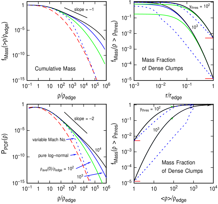
Figure 1: (Lower left) The convolution-PDF for local density in a cloud is shown as a solid curve for 3 values of the concentration ${\cal C}=\rho_{\rm ave}(0)/\rho_{\rm edge}$. The PDF develops a power-law tail with slope $3/\alpha$ for high central concentrations in a cloud with a density profile given by eq. (5). The dashed red line is a pure log-normal PDF with the same dispersion $D$ as the convolution PDF. The blue dotted line is a convolution-PDF with a variable $D$ in the log-normal part, as given by eqs. (4) and (10). (Top Left) The cumulative mass function for the same PDFs as in the bottom left, according to eq. 11. (Right panels) The fraction of the cloud mass at a density greater than the threshold density $y_{\rm thres}$ versus normalized average density (bottom) and normalized cloud radius (top). Two values of $y_{\rm thres}$ are shown, and for each, three values of ${\cal C}$ are shown (${\cal C}=10^{2}$, $10^{3}$, and $10^{4}$ for green, blue, and black curves). In the bottom panel, the 3 ${\cal C}^{\prime}s$ overlap and their endpoints are shown by appropriately colored arrows. The dotted blue curves on the right have variable $D$ with ${\cal C}=10^{3}$ and with $y_{\rm thres}=10^{2}$ and $10^{3}$, as evident from their respective proximities to the solid curves.

References

- Bate (2009) Bate, M.R. 2009, MNRAS, 392, 1363
- Bonnell & Bate (2006) Bonnell, I.A., & Bate, M.R. 2006, MNRAS, 370, 488
- Bonnell, Clark, & Bate (2008) Bonnell, I.A., Clark, P., & Bate, M.R. 2008, MNRAS, 389, 1556
- Cho & Kim (2011) Cho & Kim, 2011, MNRAS, 410, L8
- Elmegreen (2000) Elmegreen, B.G. 2000, MNRAS, 311, L5
- Elmegreen (2007) Elmegreen, B.G. 2007, ApJ, 668, 1064
- Elmegreen (2008) Elmegreen, B.G. 2008, ApJ, 672, 1006
- Elmegreen, Klessen & Wilson (2008) Elmegreen, B.G., Klessen, R., & Wilson, C. 2008, ApJ, 681, 365
- Enoch et al. (2006) Enoch, M.L. et al. 2006, ApJ, 638, 293
- Evans (2008) Evans, N.J., 2008, in Pathways through an Eclectic Universe, ASP Conf. Series Vol.390, p52
- Federrath et al. (2010) Federrath C., Roman-Duval J., Klessen R. S., Schmidt W., Mac Low M., 2010, A&A, 512, A81
- Froebrich & Rowles (2010) Froebrich, D. & Rowles, J. 2010, MNRAS, 406, 1350
- Fujimoto (1968) Fujimoto, M. 1968, ApJ, 152, 523
- Gao & Solomon (2004) Gao, Y. & Solomon, P. M. 2004, ApJ, 606, 271
- Goodwin et al. (2008) Goodwin, S.P., Nutter, D., Kroupa, P., Ward-Thompson, D., & Whitworth, A.P. 2008, A&A 477, 823
- Heiderman et al. (2010) Heiderman, A., Evans, N. J., Allen, L. E., Huard, T., & Heyer, M. 2010, ApJ, 723, 1019
- Hennebelle & Chabrier (2008) Hennebelle, P., & Chabrier, G. 2008, ApJ, 702, 142
- Hunter (1962) Hunter, C. 1962, ApJ, 136, 594
- Johnstone et al. (2000) Johnstone, D., Wilson, C.D., Moriarty-Schieven, G., Joncas, G., Smith, G., Gregersen, E., & Fich, M. 2000, 545, 327
- Johnstone et al. (2001) Johnstone, D., Fich, M., Mitchell, G.F., & Moriarty-Schieven, G. 2001, ApJ, 559, 307
- Johnstone, Di Francesco & Kirk (2004) Johnstone, D., Di Francesco, J., & Kirk, H. 2004, ApJ, 611, L45
- Kainulainen et al. (2009) Kainulainen, J., Beuther, H., Henning, T., & Plume, R. 2009, A&A, 508, L35
- Klessen (2000) Klessen, R. S. 2000, ApJ, 535, 869
- Kritsuk, Norman & Wagner (2010) Kritsuk, A.G., Norman, M.L., & Wagner, R. 2010, arXiv1007.2950
- Krumholz & Tan (2007) Krumholz, M.R., & Tan, J.C. 2007, ApJ, 654, 304
- Krumholz et al. (2010) Krumholz, M.R., Cunningham, A.J., Klein, R.I., & McKee, C.F. 2010, apJ. 713, 1120
- Lada, Lombardi & Alves (2009) Lada, C.J., Lombardi, M., & Alves, J.F. 2009, ApJ, 703, 52
- Lada, Lombardi & Alves (2010) Lada, C.J., Lombardi, M., & Alves, J.F. 2010, ApJ, 724, 687
- Lada, Evans & Falgarone (1997) Lada, E. A., Evans, N. J., & Falgarone, E. 1997, ApJ, 488, 286
- Larson (1981) Larson, R.B. 1981, MNRAS, 194, 809
- Lemaster & Stone (2008) Lemaster M. N., Stone J. M., 2008, ApJL, 682, L97
- Li et al. (2010) Li, H.-B., Blundell, R., Hedden, A., Kawamura, J., Paine, S., & Tong, E. 2010, MNRAS, tmp.1823
- Lombardi, Lada & Alves (2010) Lombardi, M., Lada, C. J., & Alves, J. 2010, A&A, 512, A67
- McKee (1989) McKee, C.F. 1989, ApJ, 345, 782
- McKee & Tan (2002) McKee, C.F., & Tan, J.C. 2002, Nature, 416, 59
- Motte, André &, Neri (1998) Motte, F., André, P., & Neri, R. 1998, A&A, 336, 150
- Padoan, Nordlund & Jones (1997) Padoan P., Nordlund A., Jones B. J. T., 1997, MNRAS, 288, 145
- Padoan & Nordlund (2002) Padoan, P., & Nordlund, A. 2002, ApJ, 576, 870
- Passot & Vázquez-Semadeni (1998) Passot, T., & Vázquez-Semadeni, E. 1998, Phys.Rev.E, 58, 4501
- Peters et al. (2010) Peters, T., Klessen, R.S., Mac Low, M.-M., & Banerjee, R. 2010, ApJ, 725, 134
- Price (2011) Price, D.J. 2011, in Computational Star Formation, IAUS 270, eds. J. Alves, B.G. Elmegreen, J.M. Girart, & V. Trimble, Cambridge University Press, in press
- Rathborne et al. (2009) Rathborne, J. M., Lada, C. J., Muench, A. A., Alves, J. F., Kainulainen, J., & Lombardi, M. 2009, ApJ, 699, 742
- Schmeja, Kumar, & Ferreira (2008) Schmeja, S., Kumar, M. S. N., & Ferreira, B. 2008, MNRAS, 389, 1209
- Shadmehri & Elmegreen (2011) Shadmehri, M., & Elmegreen, B.G. 2011, MNRAS, 410, 788
- Shu (1977) Shu, F. H. 1977, ApJ, 214, 488
- Spitzer & Jenkins (1975) Spitzer, L., Jr., & Jenkins, E.B. 1975, ARA&A, 13, 133
- Swift & Williams (2008) Swift, J.J. & Williams, J.P. 2008, ApJ, 679, 552
- Teyssier et al. (2010) Teyssier, R., Chapon, D., Bournaud, F. 2010, ApJ, 720, L149
- Vázquez-Semadeni et al (2008) Vázquez-Semadeni E., González, R.F., Ballesteros-Paredes, J., Gazol, A., & Kim, J. 2008, MNRAS, 390, 769
- Vázquez-Semadeni (1994) Vázquez-Semadeni E. 1994, ApJ, 423, 681
- Wu et al. (2005) Wu, J., Evans, N. J., Gao, Y., Solomon, P. M., Shirle, Y. L., & Vanden Bout, P. A. 2005, ApJ, 635, L173
- Wu et al. (2010) Wu, J., Evans, N. J., Shirley, Y. L., & Knez, C. 2010, ApJS, 188, 313
- Young et al. (2006) Young, K.E. et al. 2006, ApJ, 644, 326