Opportunistic Relaying for Space-Time Coded Cooperation with Multiple Antenna Terminals

Abstract

We consider a wireless relay network with multiple antenna terminals over Rayleigh fading channels, and apply distributed space-time coding (DSTC) in amplify-and-forward (A$\&$F) mode. The A$\&$F scheme is used in a way that each relay transmits a scaled version of the linear combination of the received symbols. It turns out that, combined with power allocation in the relays, A$\&$F DSTC results in an opportunistic relaying scheme, in which only the best relay is selected to retransmit the source’s space-time coded signal. Furthermore, assuming the knowledge of source-relay CSI at the source node, we design an efficient power allocation which outperforms uniform power allocation across the source antennas. Next, assuming $M$-PSK or $M$-QAM modulations, we analyze the performance of the proposed cooperative diversity transmission schemes in a wireless relay networks with the multiple-antenna source and destination. We derive the probability density function (PDF) of the received SNR at the destination. Then, the PDF is used to determine the symbol error rate (SER) in Rayleigh fading channels. We derived closed-form approximations of the average SER in the high SNR scenario, from which we find the diversity order of system $R\min\{N_{s},N_{d}\}$, where $R$, $N_{s}$, and $N_{d}$ are the number of the relays, source antennas, and destination antennas, respectively. Simulation results show that the proposed system obtain more than 6 dB gain in SNR over A&F MIMO DSTC for BER $10^{-4}$, when $R=2$, $N_{s}=2$, and $N_{d}=1$.

Index Terms— Wireless relay networks, power control, performance analysis, MIMO.

I Introduction

Space-time coding (STC) has received a lot of attention in the last decade as a way of increasing the data rate and/or reduce the transmitted power necessary to achieve a target bit error rate (BER) using multiple antenna transceivers. In ad-hoc network applications or in distributed large scale wireless networks, the nodes are often constrained in the complexity and size. This makes multiple-antenna systems impractical for certain network applications [1]. In an effort to overcome this limitation, cooperative diversity schemes have been introduced [1, 2, 3, 4]. Cooperative diversity allows a collection of radios to relay signals for each other and effectively create a virtual antenna array for combating multipath fading in wireless channels. The attractive feature of these techniques is that each node is equipped with only one antenna, creating a virtual antenna array. This property makes them outstanding for deployment in cellular mobile devices as well as in ad-hoc mobile networks, which have problems with exploiting multiple-antenna due to the size limitation of the mobile terminals.

Among the most widely used cooperative strategies are amplify-and-forward (A&F) [4], [5] and decode-and-forward (D&F) [1, 2, 4]. The authors in [6] applied Hurwitz-Radon space-time codes in wireless relay networks and conjecture a diversity factor around $R/2$ for large $R$ from their simulations, where $R$ is the number of relays.

In [7], a cooperative strategy was proposed, which achieves a diversity factor of R in a R-relay wireless network, using the so-called distributed space-time codes (DSTC). In this strategy, a two-phase protocol is used. In the first phase, the transmitter sends the information signal to the relays and in the second phase, the relays send information to the receiver. The signal sent by every relay in the second phase is designed as a linear function of its received signal. It was shown in [7] that the relays can generate a linear space-time codeword at the receiver, as in a multiple antenna system, although they only cooperate distributively. This method does not require decoding at the relays and for high SNR it achieves the optimal diversity factor [7]. Although distributed space-time coding does not need instantaneous channel information in the relays, it requires full channel information at the receiver of both the channel from the transmitter to relays and the channel from relays to the receiver. Therefore, training symbols have to be sent from both the transmitter and the relays. The design of practical A&F DSTCs that lead to reliable communication in wireless relay networks, has also been recently considered [8, 9, 10].

Distributed space-time coding was generalized to networks with multiple-antenna nodes in [11]. It was shown that in a wireless network with $N_{s}$ antennas at the transmit node, $N_{d}$ antennas at the receive node, and a total of $R$ antennas at all relay nodes, the diversity order of $R\min\{N_{s},N_{d}\}$ is achievable [11, 12]. In [13], the problem of coding design considered over wireless relay network where both the transmitter and the receiver have several antennas.

Power efficiency is a critical design consideration for wireless networks - such as ad-hoc and sensor networks - due to the limited transmission power of the nodes. To that end, choosing the appropriate relays to forward the source data, as well as the transmit power levels of the source’s antenna become important design issues. Several power allocation strategies for relay networks were studied based on different cooperation strategies and network topologies in [14]. In [15], we proposed power allocation strategies for repetition-based cooperation that take both the statistical CSI and the residual energy information into account to prolong the network lifetime while meeting the BER QoS requirement of the destination. Distributed power allocation strategies for D&F cooperative systems were investigated in [16]. Power allocation in three-node models are discussed in [17] and [18], while multi-hop relay networks are studied in [19, 20, 21]. The relay selection algorithms for networks with multiple relays can be also resulted in power efficient transmission strategies. Recently proposed practical relay selection strategies include pre-select one relay [22], best-select relay [22], blind-selection-algorithm [23], informed-selection-algorithm [23], and cooperative relay selection [24]. In [25], an opportunistic relaying scheme is introduced. According to opportunistic relaying, a single relay among a set of $R$ relay nodes is selected, depending on which relay provides for the best end-to-end path between source and destination. Bletsas et al. [25] proposed two heuristic methods for selecting the best relay based on the end-to-end instantaneous wireless channel conditions. Performance and outage analysis of these heuristic relay selection schemes were studied in [26] and [27].

In this paper, we propose decision metrics for opportunistic relaying based on maximizing the received instantaneous SNR at the destination in A&F mode, when both the source and destination have multiple-antennas. We use a simple feedback from the destination toward the relays to select the best relay and the best antenna at the source node.

Our main contributions can be summarized as follows:

• We show that the distributed space-time codes (DSTC) based on [7] in a relay network with the multiple-antennas source and destination leads to a novel opportunistic relaying, when maximum instantaneous SNR based power allocation is employed.

• Assuming the knowledge of CSI of the source-relay links at the source, the optimum power allocations along the source’s antennas based on maximizing the received SNR are derived.

• We analyze the performance of the proposed A$\&$F opportunistic relaying with space-time coded source. In addition, the performance analysis of full-opportunistic scheme is studied, in which power control for both the source antennas and the relays are employed. More specifically, we derive the average symbol error rate (SER) of opportunistic relaying and full-opportunistic schemes with $M$-PSK and $M$-QAM modulations in a Rayleigh fading channels. Furthermore, the probability density function (PDF) of the received SNR at the destination is obtained.

• For sufficiently high SNR, simple closed-form average SER expressions are derived for A$\&$F opportunistic relaying links with multiple cooperating branches and multiple antennas source/destination. Based on the proposed approximated SER expression, it is shown that the proposed schemes achieve the diversity order of $R\min\{N_{s},N_{d}\}$, where $R$, $N_{s}$, and $N_{d}$ are the number of relays, source antennas, and the destination antennas, respectively.

• We verify the obtained analytical results using simulations. The results show that the derived error rates have the same system performance as simulation results. Assuming $R=2$, $N_{s}=2$, $N_{d}=1$, the proposed opportunistic scheme outperforms DSTC by about 6 dB gain in SNR at BER $10^{-4}$.

The remainder of this paper is organized as follows: In Section II, the system model is given. The power control strategies for A&F DSTC based on the availability of CSI at the source and relays are considered in Section III. The average SER of the proposed opportunistic schemes under $M$-PSK and $M$-QAM modulations are derived in Section IV. In Section V, closed-form approximations for the average SER are presented, and the diversity analysis is carried out. In Section VI, the overall system performance is presented via simulations for different numbers of relays, source and destination antennas, and the correctness of the analytical formulas are confirmed by Monte Carlo simulations. Conclusions are presented in Section VII. The article contains four appendices which present various proofs.

Notations: The superscripts ^t and ^H stand for transposition and conjugate transposition, respectively. The expectation value operation is denoted by $\mathbb{E}\{\cdot\}$. The symbol $\boldsymbol{I}_{T}$ stands for the $T\times T$ identity matrix. $\|\boldsymbol{A}\|$ denotes the Frobenius norm of the matrix $\boldsymbol{A}$. The trace of the matrix $\boldsymbol{A}$ is denoted by $\text{tr}\left\{\boldsymbol{A}\right\}$. $\operatorname{diag}\{\boldsymbol{A}_{1},\ldots,\boldsymbol{A}_{R}\}$ denotes the block diagonal matrix.

II System Model

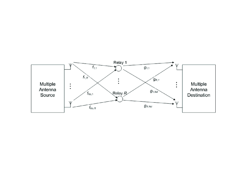
Figure 1: Wireless relay network including one source with $N_{s}$ antennas, $R$ relays, and one destination with $N_{d}$ antennas.

Consider a wireless communication scenario where the source node s transmits information to the destination node d with the assistance of one or more relays denoted Relay $r=1,2,\ldots,R$ (see Fig. 1). The source and destination nodes are equipped with $N_{s}$ and $N_{d}$ antennas, respectively. Without loss of generality, it is assumed that each relay nodes is equipped with a single antennas. Note that this network can be transformed to relays with multiple antenna, since the transmit and receive signals at different antennas of the same relay can be processed and designed independently.

We denote the links from the $N_{s}$ source antennas to the $r$th relay as $f_{1,r},f_{2,r},\ldots,f_{N_{s},r}$, and the links from the $r$th relay to the $N_{d}$ destination antennas as $g_{r,1},g_{r,2},\ldots,g_{r,N_{d}}$. Under the assumption that each link undergoes independent Rayleigh process $f_{i,r}$, and $g_{r,j}$ are independent complex Gaussian random variables with zero-mean and variances $\sigma_{f_{r}}^{2}$, and $\sigma_{g_{r}}^{2}$, respectively. Since the multiple antennas in source and destination are co-located, and the co-located antennas have the same distances to relays, we skipped the $i$ and $j$ indices of $\sigma_{f_{r}}^{2}$ and $\sigma_{g_{r}}^{2}$.

Assume that the source wants to send $K$ symbols $s_{1}$, $s_{2}$, $\ldots$, $s_{K}$ to the destination during $T$ time slots. $T$ should be less than the coherent interval, that is, the time duration among which the channels $f_{i,r}$, and $g_{r,j}$ are constant. Henceforth, we assume using full-rate space-time codes, and thus, $K=T$. Similar to [7], our scheme requires two phases of transmission. During the first phase, the source should transmit a $T\times N_{s}$ dimensional orthogonal code matrix $\boldsymbol{S}_{1}$ to all relays. We can represent $\boldsymbol{S}_{1}$ in terms of the vector $\boldsymbol{s}=[s_{1},s_{2},\ldots,s_{T}]^{t}$ as

$$\boldsymbol{S}_{1}=[\boldsymbol{A}_{1}\boldsymbol{s}\,\boldsymbol{A}_{2}\boldsymbol{s}\,\ldots\,\boldsymbol{A}_{N_{s}}\boldsymbol{s}],$$ (1)

where $\boldsymbol{A}_{i}$, $i=1,\ldots,N_{s}$, are $T\times T$ unitary matrices, and $\boldsymbol{s}_{i}=\boldsymbol{A}_{i}\boldsymbol{s}$ describes the $i$th column of a $T\times N_{s}$ orthogonal space-time code. We assume the following normalization

$$\mathbb{E}\left[\,\text{tr}\{\boldsymbol{S}_{1}^{H}\boldsymbol{S}_{1}\}\right]=\mathbb{E}\left[\,\text{tr}\left\{\sum_{k=1}^{T}|s_{k}|^{2}\boldsymbol{I}_{N_{s}}\right\}\right]=N_{s}.$$ (2)

The source transmits $\sqrt{P_{1}T/N_{s}}\boldsymbol{S}_{1}$ where $P_{1}T$ is the average total power used at the source during the first phase. Thus, $\sqrt{P_{1}T/N_{s}}\boldsymbol{s}_{i}$, $i=1,\ldots,N_{s}$, is the signal sent by the $i$th antenna with the average power of $P_{1}T/N_{s}$. Assuming that $f_{i,r}$ does not vary during $T$ successive intervals, the $T\times 1$ receive signal vector at the $r$th relay is

$$\boldsymbol{x}_{r}=\sqrt{\frac{P_{1}T}{N_{s}}}\boldsymbol{S}_{1}\boldsymbol{f}_{r}+\boldsymbol{v}_{r},$$ (3)

where $\boldsymbol{f}_{r}=[{f}_{1,r}\,{f}_{2,r}\,\ldots\,{f}_{N_{s},r}]^{t}$, and $\boldsymbol{v}_{r}$ is a $T\times 1$ complex zero-mean white Gaussian noise vector with variance $\mathcal{N}_{1}$.

In the second phase of the transmission, all relays simultaneously transmit linear functions of their received signals $\boldsymbol{x}_{r}$. In order to construct a distributed space-time codes, the received signal at the $j$th antenna of the destination is collected inside the $T\times 1$ vector $\boldsymbol{y}_{j}$ as

$$\boldsymbol{y}_{j}=\sum_{r=1}^{R}g_{r,j}\,\rho_{r}\boldsymbol{C}_{r}\boldsymbol{x}_{r}+\boldsymbol{w}_{j},$$ (4)

for $j=1,2,\ldots,N_{r}$, where $\boldsymbol{w}_{j}$ is a $T\times 1$ complex zero-mean white Gaussian noise vector with component-wise variance $\mathcal{N}_{2}$, $\rho_{r}$ is the scaling factor at Relay $r$, and $\boldsymbol{C}_{r}$, of size $T\times T$, are obtained by representing the $r$th column of an appropriate $T\times R$ dimensional space-time code matrix as $\boldsymbol{C}_{r}\boldsymbol{s}$. This construction method originates from the construction of a space-time code for co-located multiple-antenna systems, where the transmitted signal vector from the $k$th antenna is $\boldsymbol{C}_{k}\boldsymbol{s}$ [28]. When there is no instantaneous channel state information (CSI) at the relays, but statistical CSI is known, a useful constraint is to ensure that a given average transmitted power is maintained. That is,

$$\rho_{r}=\sqrt{\frac{P_{2,r}}{\sigma_{f_{r}}^{2}P_{1}+\mathcal{N}_{1}}},$$ (5)

where $P_{2,r}$ is the average transmitted power from Relay r.

We can further represent input-output relationship of the DSTC as the space-time code in a multiple-antenna system. By setting the $T\times N_{s}R$ space-time encoded signal

$$\boldsymbol{S}=[\boldsymbol{C}_{1}\boldsymbol{S}_{1},\,\boldsymbol{C}_{2}\boldsymbol{S}_{1},\,\ldots,\,\boldsymbol{C}_{R}\boldsymbol{S}_{1}],$$ (6)

and by concatenating the received signals of the destination antennas, i.e., $\boldsymbol{Y}=[\boldsymbol{y}_{1}\,\boldsymbol{y}_{2}\,\ldots\,\boldsymbol{y}_{N_{d}}]\in\mathds{C}^{T\times N_{d}}$, from (3)-(4), we have

$$\boldsymbol{Y}=\sqrt{\frac{P_{1}T}{N_{s}}}\boldsymbol{S}\boldsymbol{H}+\boldsymbol{W}_{T}.$$ (7)

The $N_{s}R\times N_{d}$ channel matrix $\boldsymbol{H}$ in (7) can be written as

$$\boldsymbol{H}=\boldsymbol{F}\boldsymbol{\Lambda}\boldsymbol{G},$$ (8)

where matrices $\boldsymbol{F}$, $\boldsymbol{\Lambda}$, and $\boldsymbol{G}$ of sizes $N_{s}R\times R$, $R\times R$, $R\times N_{d}$, respectively, are given by

$$\boldsymbol{F}=\operatorname{diag}\left\{\boldsymbol{f}_{1},\ldots,\boldsymbol{f}_{R}\right\},\,\,\,\,\,\,\,\,\,\boldsymbol{\Lambda}=\operatorname{diag}\left\{\rho_{1},\ldots,\rho_{R}\right\},$$

$$\boldsymbol{g}_{r}=[{g}_{r,1}\,{g}_{r,2}\,\ldots\,{g}_{r,N_{d}}],\,\,\,\,\,\,\,\,\,\boldsymbol{G}=\left[\boldsymbol{g}_{1}^{t},\ldots,\boldsymbol{g}_{R}^{t}\right]^{t}.$$

The total noise in (7) is collected into the $T\times N_{d}$ matrix

$$\boldsymbol{W}_{T}=\boldsymbol{V}\boldsymbol{\Lambda}\boldsymbol{G}+\boldsymbol{W},$$ (9)

where $\boldsymbol{V}=\left[\boldsymbol{C}_{1}\boldsymbol{v}_{1}\,\boldsymbol{C}_{2}\boldsymbol{v}_{2}\,\ldots\,\boldsymbol{C}_{R}\boldsymbol{v}_{R}\,\right]\in\mathds{C}^{T\times R}$ and $\boldsymbol{W}=\left[\boldsymbol{w}_{1}\,\boldsymbol{w}_{2}\,\ldots\,\boldsymbol{w}_{N_{d}}\,\right]\in\mathds{C}^{T\times N_{d}}$.

Since in this paper, we focus on orthogonal design, the maximum likelihood (ML) detection is decomposed to single-symbol detection, maximal-ratio combining (MRC) can be applied at the destination [29]. To calculate the post detection SNR at the output of the ML DSTC decoder, we need to compute the received signal power. Hence, using (7), we have

$$\eta_{{s}_{d}} =\frac{P_{1}T}{N_{s}}\mathbb{E}_{s}\!\left[\text{tr}\{\boldsymbol{S}\boldsymbol{H}\boldsymbol{H}^{H}\boldsymbol{S}^{H}\}\right]\!=\!\frac{P_{1}T}{N_{s}}\mathbb{E}_{s}\!\left[\text{tr}\{\boldsymbol{H}\boldsymbol{H}^{H}\boldsymbol{S}^{H}\boldsymbol{S}\}\right]=\frac{P_{1}T}{N_{s}}\,\text{tr}\{\boldsymbol{H}\boldsymbol{H}^{H}\,\mathbb{E}_{s}[\boldsymbol{S}^{H}\boldsymbol{S}]\}.$$ (10)

To have the linear orthogonal ML detection, we should design the DSTC, such that

$$\boldsymbol{S}^{H}\boldsymbol{S}=(|s_{1}|^{2}+|s_{2}|^{2}+\ldots+|s_{T}|^{2})\boldsymbol{I}_{N_{s}R},$$ (11)

and using the normalization assumed in (2), we have $\mathbb{E}_{s}[\boldsymbol{S}^{H}\boldsymbol{S}]=\boldsymbol{I}_{N_{s}R}$. For designing the distributed orthogonal space-time codes in multiple-antenna relay netowrks, one can see [30]. Thus, $\eta_{{s}_{d}}$ in (10) can be evaluated as

$$\eta_{{s}_{d}} =\frac{P_{1}T}{N_{s}}\,\text{tr}\{\boldsymbol{H}\boldsymbol{H}^{H}\}=\frac{P_{1}T}{N_{s}}\,\sum_{i=1}^{N_{s}R}\left[\boldsymbol{H}\boldsymbol{H}^{H}\right]_{i,i}$$

$$=\frac{P_{1}T}{N_{s}}\!\sum_{r=1}^{R}\!\sum_{n=1}^{N_{s}}|f_{n,r}|^{2}\rho_{r}^{2}\sum_{j=1}^{N_{d}}|g_{r,j}|^{2}=\frac{P_{1}T}{N_{s}}\!\sum_{r=1}^{R}\rho_{r}^{2}\|\boldsymbol{f}_{r}\|^{2}\|\boldsymbol{g}_{r}\|^{2}.$$ (12)

From (9), and assuming $\boldsymbol{C}_{r}$, $r=1,\ldots,R$ are unitary matrices, the total noise power at the destination can be written as

$$\eta_{{w}_{T}}=\mathbb{E}_{v,w}[\text{tr}\{\boldsymbol{W}_{T}\boldsymbol{W}_{T}^{H}\}]=T\left(\sum_{k=1}^{R}\rho_{k}^{2}\|\boldsymbol{g}_{k}\|^{2}\mathcal{N}_{1}+N_{d}\mathcal{N}_{2}\right).$$ (13)

Combining (II) and (13), the received SNR at the destination can be written as

$$\text{SNR}_{\text{ins}}=\sum_{r=1}^{R}\frac{P_{1}\rho_{r}^{2}\|\boldsymbol{f}_{r}\|^{2}\|\boldsymbol{g}_{r}\|^{2}}{N_{s}\displaystyle\sum_{k=1}^{R}\rho_{k}^{2}\|\boldsymbol{g}_{k}\|^{2}\mathcal{N}_{1}+N_{s}N_{d}\mathcal{N}_{2}}.$$ (14)

III Power Control in A$\&$F Space-Time Coded Cooperation

In this section, we propose power allocation schemes for the A$\&$F distributed space-time codes with multiple antennas source/destination, based on maximizing the received SNR at the destination d. First, we will find the optimum distribution of transmitted powers among relays, i.e., $P_{2,r}$, based on instantaneous SNR. Then, the optimum power transmitted in the two phases, i.e., $P_{1}$ and $P_{2}=\sum_{r=1}^{R}P_{2,r}$, will be obtained by maximizing the average received SNR at the destination.

III-A Power Control among Relays with No CSI at the Source

Here, we find the optimum distribution of the transmitted powers among relays during the second phase, in a sense of maximizing the instantaneous SNR at the destination.

III-A1 Optimum Power Allocation

Using (5) and (14), the instantaneous received SNR at the destination can be written as

$$\text{SNR}_{\text{ins}}=\frac{\boldsymbol{p}^{t}\boldsymbol{U}\boldsymbol{p}}{\boldsymbol{p}^{t}\boldsymbol{Q}\boldsymbol{p}+N_{s}N_{d}\mathcal{N}_{2}},$$ (15)

where $\boldsymbol{p}=[\sqrt{P_{2,1}},\sqrt{P_{2,2}},\ldots,\sqrt{P_{2,R}}]^{t}$ and diagonal $R\times R$ matrices $\boldsymbol{U}$ and $\boldsymbol{V}$ are defined as

$$\boldsymbol{U} \!\!=\!\operatorname{diag}\!\!\left[\!\frac{P_{\!1}\|\boldsymbol{f}_{\!1}\|^{2}\|\boldsymbol{g}_{\!1}\|^{2}}{\sigma_{f_{1}}^{2}P_{1}+\mathcal{N}_{1}},\frac{P_{\!1}\|\boldsymbol{f}_{\!2}\|^{2}\|\boldsymbol{g}_{\!2}\|^{2}}{\sigma_{f_{2}}^{2}P_{1}+\mathcal{N}_{1}},\ldots,\frac{P_{\!1}\|\boldsymbol{f}_{\!\!R}\|^{2}\|\boldsymbol{g}_{\!R}\|^{2}}{\sigma_{f_{R}}^{2}P_{1}+\mathcal{N}_{1}}\!\right]\!,$$

$$\boldsymbol{Q} =\operatorname{diag}\left[\frac{N_{s}\|\boldsymbol{g}_{1}\|^{2}\mathcal{N}_{1}}{\sigma_{f_{1}}^{2}P_{1}+\mathcal{N}_{1}},\frac{N_{s}\|\boldsymbol{g}_{2}\|^{2}\mathcal{N}_{1}}{\sigma_{f_{2}}^{2}P_{1}+\mathcal{N}_{1}},\ldots,\frac{N_{s}\|\boldsymbol{g}_{R}\|^{2}\mathcal{N}_{1}}{\sigma_{f_{R}}^{2}P_{1}+\mathcal{N}_{1}}\right].$$ (16)

Then, the optimization problem is formulated as

$$\boldsymbol{p}^{*}=\arg\max_{\boldsymbol{p}}\text{SNR}_{\text{ins}},\,\,\,\,\text{subject to}\,\,\,\,\boldsymbol{p}^{t}\boldsymbol{p}=P_{2},$$ (17)

where the $R\times 1$ vector $\boldsymbol{p}^{*}$ denotes the optimum values of power control coefficients. Since $\boldsymbol{p}^{t}\boldsymbol{p}=P_{2}$, we can rewrite (15) as $\text{SNR}_{\text{ins}}=\frac{\boldsymbol{p}^{t}\boldsymbol{U}\boldsymbol{p}}{\boldsymbol{p}^{t}\boldsymbol{W}\boldsymbol{p}}$, where diagonal matrix $\boldsymbol{W}$ is defined as $\boldsymbol{W}=\boldsymbol{Q}+\frac{N_{s}N_{d}\mathcal{N}_{2}}{P_{2}}\boldsymbol{I}_{T}$. Since $\boldsymbol{W}$ is a real-valued positive semi-definite matrix, we define $\boldsymbol{q}\triangleq\boldsymbol{W}^{\frac{1}{2}}\boldsymbol{p}$, where $\boldsymbol{W}=(\boldsymbol{W}^{\frac{1}{2}})^{t}\boldsymbol{W}^{\frac{1}{2}}$. Then, $\text{SNR}_{\text{ins}}$ can be rewritten as

$$\text{SNR}_{\text{ins}}=\frac{\boldsymbol{q}^{t}\boldsymbol{Z}\boldsymbol{q}}{\boldsymbol{q}^{t}\boldsymbol{q}},$$ (18)

where diagonal matrix $\boldsymbol{Z}$ is $\boldsymbol{Z}=\boldsymbol{U}\boldsymbol{W}^{-1}$. Now, using Rayleigh-Ritz theorem [31], we have

$$\frac{\boldsymbol{q}^{t}\boldsymbol{Z}\boldsymbol{q}}{\boldsymbol{q}^{t}\boldsymbol{q}}\leq\lambda_{\max},$$ (19)

where $\lambda_{\max}$ is the largest eigenvalue of $\boldsymbol{Z}$, which is corresponding to the largest diagonal element of $\boldsymbol{Z}$, i.e.,

$$\lambda_{\max}\! =\!\max_{i\in\{1,\ldots,R\}}\!\!\lambda_{i}=\!\max_{i\in\{1,\ldots,R\}}\frac{P_{1}P_{2}\|\boldsymbol{f}_{i}\|^{2}\|\boldsymbol{g}_{i}\|^{2}}{P_{2}N_{s}\|\boldsymbol{g}_{i}\|^{2}\!\mathcal{N}_{1}\!+\!N_{s}N_{d}\mathcal{N}_{2}(\sigma_{f_{i}}^{2}P_{1}\!+\!\mathcal{N}_{1}\!)}.$$ (20)

The equality in $\frac{\boldsymbol{q}^{t}\boldsymbol{Z}\boldsymbol{q}}{\boldsymbol{q}^{t}\boldsymbol{q}}=\lambda_{\max}$ holds if $\boldsymbol{q}$ is proportional to the eigenvector of $\boldsymbol{Z}$ corresponding to $\lambda_{\max}$. Using the eigenvalue decomposition of the diagonal matrix $\boldsymbol{Z}$, which contains positive diagonal elements, it is obvious that the matrix which is consisting of the normalized eigenvectors, is the identity matrix. Hence, the optimum $\boldsymbol{q}_{\max}$ is proportional to $\boldsymbol{e}_{i_{\max}}$, which is a $R\times 1$ vector with only zero elements, except one at the $i_{\max}$-th component. On the other hand, since $\boldsymbol{p}=\boldsymbol{W}^{-\frac{1}{2}}\boldsymbol{q}$, and $\boldsymbol{W}$ is a diagonal matrix, the optimum $\boldsymbol{p}^{*}$ is also proportional to $\boldsymbol{e}_{i_{\max}}$. Using the power constraint of the transmitted power in the second phase, i.e., $\boldsymbol{p}^{t}\boldsymbol{p}=P_{2}$, we have $\boldsymbol{p}^{*}=\sqrt{P_{2}}\boldsymbol{e}_{i_{\max}}$. This means that for each realization of the network channels, the best relay should transmit all the available power $P_{2}$, while all the other relays should stay silent.

III-A2 Relay Selection Strategy

The process of selecting the best relay could be done by the destination. This is feasible since the destination node should be aware of both the backward and forward channels for coherent decoding. Thus, the same channel information could be exploited for the purpose of relay selection. However, if we assume a distributed relay selection algorithm, in which relays independently decide to select the best relay among them, such as work done in [25], the knowledge of local channels $f_{i}$ and $g_{i}$ is required for the $i$th relay. The estimation of $f_{i}$ and $g_{i}$ can be done by transmitting a ready-to-send (RTS) packet and a clear-to-send (CTS) packet in MAC protocols.

III-B Power Allocation with Partial CSI at the Source

Here, we study the situation in which the CSI of the source-relay links are known at the source node. In this case, instead of uniform power allocation used in the previous subsection, power allocation is used over the transmit antennas. Thus, (3) can be rewritten as

$$\boldsymbol{x}_{r}=\sqrt{T}\boldsymbol{X}_{\!p}\boldsymbol{f}_{r}+\boldsymbol{v}_{r},$$ (21)

where $\boldsymbol{X}_{\!p}=[P_{1,1}\boldsymbol{A}_{1}\boldsymbol{s}\,P_{1,2}\boldsymbol{A}_{2}\boldsymbol{s}\,\ldots\,P_{1,N_{s}}\boldsymbol{A}_{N_{s}}\boldsymbol{s}]$, $\sum_{k=1}^{N_{s}}P_{1,k}=P_{1}$, and $P_{1,k}$, $k=1,\ldots,N_{s}$, is the transmit power from the $k$th source antenna.

Hence, using (4)-(7) and (21), $\eta_{{s}_{d}}$ in (10) can be rewritten as

$$\eta_{{s}_{d}} =T\mathbb{E}_{s}\!\left[\text{tr}\{\boldsymbol{S}_{p}\boldsymbol{H}\boldsymbol{H}^{H}\boldsymbol{S}_{p}^{H}\}\right]\!=\!T\mathbb{E}_{s}\!\left[\text{tr}\{\boldsymbol{H}\boldsymbol{H}^{H}\boldsymbol{S}_{p}^{H}\boldsymbol{S}_{p}\}\right]=T\,\text{tr}\{\boldsymbol{H}\boldsymbol{H}^{H}\,\mathbb{E}_{s}[\boldsymbol{S}_{p}^{H}\boldsymbol{S}_{p}]\},$$ (22)

where

$$\boldsymbol{S}_{p}=[ P_{1,1}\boldsymbol{C}_{1}\boldsymbol{A}_{1}\boldsymbol{s},\,\ldots,P_{1,N_{s}}\boldsymbol{C}_{1}\boldsymbol{A}_{N_{s}}\boldsymbol{s},\,\ldots,P_{1,1}\boldsymbol{C}_{R}\boldsymbol{A}_{1}\boldsymbol{s},\ldots,P_{1,N_{s}}\boldsymbol{C}_{R}\boldsymbol{A}_{N_{s}}\boldsymbol{s}],$$ (23)

has the size $T\times N_{s}R$ and using the normalization assumed in (2), we have

$$\mathbb{E}_{s}[\boldsymbol{S}_{p}^{H}\boldsymbol{S}_{p}]=\operatorname{diag}(P_{1,1},\ldots,P_{1,N_{s}})\otimes\boldsymbol{I}_{R},$$ (24)

where $\otimes$ is Kroncker product. Thus, $\eta_{{s}_{d}}$ can be evaluated as

$$\eta_{{s}_{d}} =T\sum_{r=0}^{R-1}\sum_{n=1}^{N_{s}}P_{1,n}\left[\boldsymbol{H}\boldsymbol{H}^{H}\right]_{N_{s}r+n,N_{s}r+n}=T\!\sum_{r=1}^{R}\!\sum_{n=1}^{N_{s}}P_{1,n}|f_{n,r}|^{2}\rho_{r}^{2}\|\boldsymbol{g}_{r}\|^{2}.$$ (25)

III-B1 Optimum Power Allocation

For deriving the optimum value of power in a sense of minimizing the received SNR, we have to compute $\text{SNR}_{\text{ins}}=\frac{\eta_{{s}_{d}}}{\eta_{w}}$. Combining (13) and (25), the received SNR at the destination can be written as $\text{SNR}_{\text{ins}}=\sum_{n=1}^{N_{s}}\theta_{n}P_{1,n}$ where

$$\theta_{n}=\frac{\sum_{r=1}^{R}|f_{n,r}|^{2}\rho_{r}^{2}\|\boldsymbol{g}_{r}\|^{2}}{N_{d}\sum_{k=1}^{R}\rho_{k}\|\boldsymbol{g}_{k}\|^{2}\mathcal{N}_{1}+N_{d}\mathcal{N}_{2}}.$$ (26)

Hence, we can formulate the following problem to find the optimum values of $P_{1,n}$:

$$\max\,\,\sum_{n=1}^{N_{s}}\theta_{n}P_{1,n},$$

$$\text{s.t.}\,\,\,\sum_{n=1}^{N_{s}}P_{1,n}\leq P_{1},$$

$$\,\,\,\,\,\,\,\,\,\,\,0\leq P_{1,n},\,\,\text{for}\,\,n=1,\ldots,N.$$ (27)

The optimization problem in (III-B1) is a maximal assignment problem, and it is easy to show that the solution to this problem is

$$P_{1,n}^{*}=\left\{\begin{array}[]{cc}P_{1},&\text{if}\,\,n=\arg\displaystyle\max_{i\in\{1,\ldots,N_{s}\}}\theta_{i},\\ 0,&\text{otherwise}.\\ \end{array}\right.$$ (30)

Therefore, the optimum solution for the problem stated in (III-B1) is such that the whole power in the first phase is transmitted by an antenna at the source with the highest value of $\theta_{n}$ in (26). From (30), we can rewrite the received SNR as $\text{SNR}_{\text{ins}}=\sum_{r=1}^{R}\zeta_{r}$ where

$$\zeta_{r}=\frac{P_{1}P_{2,r}\displaystyle\max_{n\in\{1,\ldots,N_{s}\}}|f_{n,r}|^{2}\|\boldsymbol{g}_{r}\|^{2}}{P_{2}\|\boldsymbol{g}_{r}\|^{2}\!\mathcal{N}_{1}\!+\!N_{d}\mathcal{N}_{2}(\sigma_{\xi_{r}}^{2}P_{1}\!+\!\mathcal{N}_{1}\!)}.$$ (31)

Now, by defining $\xi_{r}=\max_{n\in\{1,\ldots,N_{s}\}}|f_{n,r}|^{2}$ with mean $\sigma_{\xi_{r}}^{2}$, we can employ a similar procedure used in the previous subsection to find the optimal values of $P_{2,r}$, and the matrices $\boldsymbol{U}$ and $\boldsymbol{Q}$ in (III-A1) are redefined as

$$\boldsymbol{U} \!\!=\!\operatorname{diag}\!\!\left[\!\frac{P_{\!1}\xi_{1}\|\boldsymbol{g}_{\!1}\|^{2}}{\sigma_{\xi_{1}}^{2}P_{1}+\mathcal{N}_{1}},\frac{P_{\!1}\xi_{2}\|\boldsymbol{g}_{2}\|^{2}}{\sigma_{\xi_{2}}^{2}P_{1}+\mathcal{N}_{1}},\ldots,\frac{P_{\!1}\xi_{\!R}\|\boldsymbol{g}_{\!R}\|^{2}}{\sigma_{\xi_{R}}^{2}P_{1}+\mathcal{N}_{1}}\!\right]\!,$$

$$\boldsymbol{Q} =\operatorname{diag}\left[\frac{N_{s}\|\boldsymbol{g}_{1}\|^{2}\mathcal{N}_{1}}{\sigma_{\xi_{1}}^{2}P_{1}+\mathcal{N}_{1}},\frac{N_{s}\|\boldsymbol{g}_{2}\|^{2}\mathcal{N}_{1}}{\sigma_{\xi_{2}}^{2}P_{1}+\mathcal{N}_{1}},\ldots,\frac{N_{s}\|\boldsymbol{g}_{R}\|^{2}\mathcal{N}_{1}}{\sigma_{\xi_{R}}^{2}P_{1}+\mathcal{N}_{1}}\right].$$ (32)

Therefore, similar to (20), the whole transmission power should be sent from a best relay in the optimal setting. The relay with highest value of $\frac{P_{1}\displaystyle\xi_{j}\|\boldsymbol{g}_{j}\|^{2}}{P_{2}\|\boldsymbol{g}_{j}\|^{2}\!\mathcal{N}_{1}\!+\!N_{d}\mathcal{N}_{2}(\sigma_{\xi_{j}}^{2}\!P_{1}\!+\!\mathcal{N}_{1}\!)}$ is selected as the best relay, and its corresponding power is chosen as

$$P_{2,r}^{*}=\left\{\begin{array}[]{cc}P_{2},&\text{if}\,\,r=\arg\!\!\displaystyle\max_{j\in\{1,\ldots,R\}}\!\frac{P_{1}\displaystyle\xi_{j}\|\boldsymbol{g}_{j}\|^{2}}{P_{2}\|\boldsymbol{g}_{j}\|^{2}\!\mathcal{N}_{1}\!+\!N_{d}\mathcal{N}_{2}(\sigma_{\xi_{j}}^{2}\!P_{1}\!+\!\mathcal{N}_{1}\!)},\\ 0,&\text{otherwise}.\\ \end{array}\right.$$ (35)

III-B2 Relay and Source Antenna Selection Strategy

Based on (30) and (35), we can summarize the process of relay and source’s antenna selection as follows:
(1) Choose the best relay such that $r^{*}=\arg\displaystyle\max_{r\in\{1,\ldots,R\}}\frac{\displaystyle\max_{n\in\{1,\ldots,N_{s}\}}|f_{n,r}|^{2}\|\boldsymbol{g}_{r}\|^{2}}{P_{2}\|\boldsymbol{g}_{r}\|^{2}\!\mathcal{N}_{1}\!+\!N_{d}\mathcal{N}_{2}(\sigma_{\xi_{r}}^{2}\!P_{1}\!+\!\mathcal{N}_{1}\!)}$.
(2) After finding $r^{*}$, choose the $n^{*}$th antenna at the source as the best antenna, such that $n^{*}=\arg\displaystyle\max_{n\in\{1,\ldots,N_{s}\}}|f_{n,r^{*}}|^{2}$.

III-C Power Allocation with CSI at the Source and No CSI at Relays

Here, we study the situation in which the CSI of the source-relay links are known at the source node, when no power allocation is used at the relays. In this case, we employ DSTC with uniform power allocation at the relays.

From (26) and by assuming the equal power allocation among relays is used, i.e., $P_{2,r}=P_{2}$, $r=1,\ldots,R$, we have $\text{SNR}_{\text{ins}}=\sum_{n=1}^{N_{s}}P_{1,n}\theta_{n}$ where $\theta_{n}$ can be rewritten as

$$\theta_{n}=\frac{\sum_{r=1}^{R}|f_{n,r}|^{2}\frac{P_{2}}{\sigma_{f_{n^{\!*}\!,r}}^{2}\!P_{1}\!+\!\mathcal{N}_{1}}\|\boldsymbol{g}_{r}\|^{2}}{N_{d}\sum_{k=1}^{R}\frac{P_{2}}{\sigma_{f_{n^{\!*}\!,k}}^{2}\!P_{1}\!+\!\mathcal{N}_{1}}\|\boldsymbol{g}_{k}\|^{2}\mathcal{N}_{1}+N_{d}\mathcal{N}_{2}},$$ (36)

where $\sigma_{f_{n^{\!*}\!,r}}^{2}$ is the mean of the random variable $|f_{n^{*},r}|^{2}$, and $n^{*}$ denotes the index of the selected antenna at the source.

Similar to the optimization problem stated in (III-B1), we can find the optimal value of $P_{1,n}$ from (30). Moreover, by defining $\tilde{\theta}_{n}$ as

$$\tilde{\theta}_{n}=\sum_{r=1}^{R}\frac{|f_{n,r}|^{2}\|\boldsymbol{g}_{r}\|^{2}}{\sigma_{f_{n^{\!*}\!,r}}^{2}\!P_{1}\!+\!\mathcal{N}_{1}},$$ (37)

we can equivalently find the optimal value of $P_{1,n}$ given by

$$P_{1,n}^{*}=\left\{\begin{array}[]{cc}P_{1},&\text{if}\,\,n=\arg\displaystyle\max_{i\in\{1,\ldots,N_{s}\}}\tilde{\theta}_{i}\\ 0,&\text{otherwise}\\ \end{array}\right.$$ (40)

Therefore, the whole power in the first phase is transmitted by the antenna at the source with the highest value of $\tilde{\theta}_{n}=\sum_{r=1}^{R}\frac{|f_{n,r}|^{2}\|\boldsymbol{g}_{r}\|^{2}}{\sigma_{f_{n^{\!*}\!,r}}^{2}\!P_{1}\!+\!\mathcal{N}_{1}}$. The transmission power $P_{2}$ in the second phase can be chosen equally as $\frac{P}{2R}$.

Note that the process selection of the best antenna at the source can be done at the destination in which we have access to the CSI. Then, the index of the selected antenna at the source is fed back to the source.

III-D Power Control between Two Phases

In the following proposition, we derive the optimal value for the transmitted power in the two phases when backward and forward channels have different variances by maximizing the average SNR at the destination.

Proposition 1

Assume $\tau$ portion of the total power is transmitted in the first phase and the remaining power is transmitted by relays at the second phase, where $0<\tau<1$, that is $P_{1}=\tau P$ and $P_{2}=(1-\tau)P$, where $P$ is the total transmitted power during two phases. Assuming $\sigma_{f_{r}}^{2}=\sigma_{f}^{2}$ and $\sigma_{g_{r}}^{2}=\sigma_{g}^{2}$, the optimum value of $\tau$ by maximizing the average SNR at the destination is

$$\tau=\frac{\mathcal{N}_{1}\sigma_{g}^{2}P+\mathcal{N}_{1}\mathcal{N}_{2}}{(\mathcal{N}_{2}\sigma_{f}^{2}-\mathcal{N}_{1}\sigma_{g}^{2})\,P}\left(\sqrt{1+\frac{(\mathcal{N}_{2}\sigma_{f}^{2}-\mathcal{N}_{1}\sigma_{g}^{2})\,P}{\mathcal{N}_{1}\sigma_{g}^{2}P+\mathcal{N}_{1}\mathcal{N}_{2}}}-1\right).$$ (41)

Proof:

The proof is given in Appendix I. ∎

For the special case of $\mathcal{N}_{2}\sigma_{f}^{2}=\mathcal{N}_{1}\sigma_{g}^{2}$, it can be seen from (41) that $\displaystyle\lim_{\delta\rightarrow 0}\frac{1}{\delta}(\sqrt{1+\delta}-1)=\frac{1}{2}$, where $\delta=\frac{(\mathcal{N}_{2}\sigma_{f}^{2}-\mathcal{N}_{1}\sigma_{g}^{2})\,P}{\mathcal{N}_{1}\sigma_{g}^{2}P+\mathcal{N}_{1}\mathcal{N}_{2}}$. Hence, the optimum $\tau$ is equal to $\frac{1}{2}$, which is in compliance with the result obtained in [7] where assumed $\mathcal{N}_{1}=\mathcal{N}_{2}$ and $\sigma_{f}^{2}=\sigma_{g}^{2}$.

IV Performance Analysis

IV-A SER Expression of Relay Network with No CSI at the Source

In the previous section, we have shown that the optimum transmitted power of A$\&$F DSTC system based on maximizing the instantaneous received SNR at the destination led to opportunistic relaying. In this section, we will derive the SER formulas of best relay selection strategy using A&F. For this reason, we should first derive the PDF of the received SNR at the destination due to the $r$th relay, when other relays are silent, that is

$$\gamma_{r}=\frac{P_{1}P_{2}\|\boldsymbol{f}_{r}\|^{2}\|\boldsymbol{g}_{r}\|^{2}}{P_{2}N_{s}\|\boldsymbol{g}_{r}\|^{2}\!\mathcal{N}_{1}\!+\!N_{s}N_{d}\mathcal{N}_{2}(\sigma_{f_{r}}^{2}P_{1}\!+\!\mathcal{N}_{1}\!)}.$$ (42)

Now, we will derive the PDF of $\gamma_{r}$, which is required for calculating the average SER.

Proposition 2

For $\gamma_{r}$ in (42), the PDF $p_{r}(\gamma)$ can be written as

$$p_{r}(\gamma) \!=\!\sum_{k=0}^{N_{s}}\!\frac{2a^{k}\overline{Y}_{\!r}^{k}\!{N_{s}\choose k}e^{-\frac{a\gamma}{\overline{X}_{\!r}}}}{\gamma\,(N_{d}\!\!-\!\!1)!\,(N_{s}\!\!-\!\!1)!\,b_{r}^{k}}\!\left(\!\frac{b_{r}\gamma}{\overline{X}_{\!r}\!\overline{Y}_{\!r}}\!\right)^{\!\!\!\frac{\mu+k}{2}}\!\!\!\!\!K_{\nu+k}\!\!\left(\!2\sqrt{\!\frac{b_{r}\gamma}{\overline{X}_{\!r}\!\overline{Y}_{\!r}}}\right)\!,$$ (43)

where $\mu=N_{s}+N_{d}$, $\nu=N_{d}-N_{s}$, $\overline{X}_{\!r}=N_{s}\sigma_{f_{r}}^{2}$, $\overline{Y}_{\!r}=N_{d}\sigma_{g_{r}}^{2}$, $a=\frac{N_{s}\mathcal{N}_{1}}{P_{1}}$, $b_{r}=\frac{N_{s}N_{d}\mathcal{N}_{2}(\sigma_{f_{r}}^{2}P_{1}+\mathcal{N}_{1})}{P_{1}P_{2}}$, $K_{n}(x)$ is the modified Bessel function of the second kind of order $n$.

Proof:

The proof is given in Appendix II. ∎

Define $\gamma_{\max}\triangleq\max\left\{\gamma_{1},\gamma_{2},\ldots,\gamma_{R}\right\}$. The conditional SER of the best relay selection system under A$\&$F mode with R relays can be written as

$$P_{e}\left(R|\boldsymbol{F},\boldsymbol{G}\right)=c\,Q\left(\sqrt{g\,\gamma_{\max}}\right),$$ (44)

where $Q(x)=1/\sqrt{2\pi}\int_{x}^{\infty}e^{-u^{2}/2}\,du$, and parameters $c$ and $g$ are represented as

$$c_{\text{QAM}}\!=\!4\frac{\sqrt{M}-1}{\sqrt{M}},\,\,c_{\text{PSK}}\!=\!2,\,\,g_{\text{QAM}}\!=\!\frac{3}{M-1},\,\,g_{\text{PSK}}\!=\!2\sin^{2}\!\!\left(\!\frac{\pi}{M}\!\right).$$

Using the result from order statistics, and by assuming that all channel coefficients are independent of each other, the PDF of $\gamma_{\max}$ can be written as

$$p_{\max}(\gamma)=\sum_{r=1}^{R}p_{r}(\gamma){\prod_{\underset{j\neq r}{j=1}}^{R}}\text{Pr}\{\gamma_{j}<\gamma\},$$ (45)

where $\text{Pr}\{\gamma_{j}<\gamma\}$ can be evaluated as

$$\text{Pr}\{\gamma_{j}<\gamma\}=\text{Pr}\{XY/(aY+b_{j})<\gamma\}$$

$$=\int_{0}^{\infty}\left(1-e^{-\frac{x}{\overline{X}_{\!j}}}\sum_{n=0}^{N_{s}-1}\frac{1}{n!}\left(\frac{x}{\overline{X}_{\!j}}\right)^{\!\!n}\right)\frac{y^{N_{d}-1}}{(N_{d}-1)!\,\overline{Y}_{\!j}^{N_{d}}}e^{-\frac{y}{\overline{Y}_{\!j}}}dy$$

$$=1-\int_{0}^{\infty}\sum_{n=0}^{N_{s}-1}\left(\frac{\gamma(ay+b_{j})}{y\overline{X}_{j}}\right)^{\!\!n}\frac{e^{-\frac{\gamma(ay+b_{j})}{y\overline{X}_{j}}}y^{N_{d}-1}}{n!\,(N_{d}-1)!\,\overline{Y}_{j}^{N_{d}}}e^{-\frac{y}{\overline{Y}_{j}}}dy$$

$$=1\!-\!\!\sum_{n=0}^{N_{s}\!-\!1}\!\sum_{k=0}^{n}\!\frac{{n\choose k}a^{k}b_{j}^{n-k}\gamma^{n}e^{-\frac{a\gamma}{\overline{X}_{\!j}}}}{n!\,(N_{d}\!-\!1)!\,\overline{X}_{\!j}^{n}\overline{Y}_{\!j}^{N_{d}}}\!\int_{0}^{\infty}\!\!\!\!y^{N_{d}+k-n-1}e^{-\frac{y}{\overline{Y}_{\!j}}-\frac{b_{j}\gamma}{y\overline{X}_{\!j}}}dy$$

$$=\!1\!-\!\!\!\sum_{n=0}^{N_{s}\!-\!1}\!\sum_{k=0}^{n}\!\!\frac{2{n\choose k}a^{k}\overline{Y}_{\!j}^{k}e^{-\frac{a\gamma}{\overline{X}_{\!j}}}}{n!\,(N_{d}\!-\!1)!\,b_{j}^{k}}\!\left(\!\frac{b_{j}\gamma}{\overline{X}_{\!j}\!\overline{Y}_{\!j}}\!\right)^{\!\!\!\frac{N_{d}+n+k}{2}}\!\!\!\!\!\!\!\!\!K_{\!N_{d}-n+k}\!\!\left(\!2\sqrt{\!\frac{b_{j}\gamma}{\overline{X}_{\!j}\!\overline{Y}_{\!j}}}\right)\!,$$ (46)

where $x=\frac{\gamma(ay+b_{j})}{y\overline{X}_{\!j}}$, and in the second equality, we used the Erlang distribution [32, Eq. (3.48)].

Now, we are deriving the SER expression for the selection relaying scheme discussed in Section III. Averaging over conditional SER $P_{e}\left(R|\boldsymbol{F},\boldsymbol{G}\right)$, we have the exact SER expression as

$$P_{e}(R) =\int_{0}^{\infty}P_{e}\left(R|\boldsymbol{F},\boldsymbol{G}\right)\,p_{\max}(\gamma)\,d\gamma$$

$$=\int_{0}^{\infty}c\,Q\left(\sqrt{g\,\gamma}\right)\,p_{\max}(\gamma)\,d\gamma.$$ (47)

IV-B SER Expression of Relay Network with Partial CSI at the Source

In this subsection, we will derive the SER formulas of the best relay selection strategy under the amplify-and-forward mode, when the source-relays CSI are available at the source. For this reason, we should first derive the PDF of the received SNR at the destination due to the $r$th relay, when other relays are silent. That is, from (30), (31), and (35), we can rewrite $\text{SNR}_{\text{ins}}=\sum_{r=1}^{R}\zeta_{r}$ as $\text{SNR}_{\text{ins}}=\max_{r\in\{1,\ldots,R\}}\zeta_{r}$ where

$$\zeta_{r}=\frac{P_{1}P_{2}\displaystyle\max_{n\in\{1,\ldots,N_{s}\}}|f_{n,r}|^{2}\|\boldsymbol{g}_{r}\|^{2}}{P_{2}\|\boldsymbol{g}_{r}\|^{2}\!\mathcal{N}_{1}\!+\!N_{d}\mathcal{N}_{2}(\sigma_{\xi_{r}}^{2}P_{1}\!+\!\mathcal{N}_{1}\!)}.$$ (48)

In the following, we will derive the PDF of $\zeta_{r}$, which is required for calculating the average SER.

Proposition 3

For $\zeta_{r}$ in (31), the probability density function $p_{\zeta_{r}}(\zeta)$ can be written as

$$p_{\zeta_{r}}(\zeta)\!= \!\sum_{k=1}^{N_{s}}\!\frac{2(-1)^{k+1}\!{N_{s}\choose k}k\,\alpha\,e^{-\frac{\alpha\zeta k}{\sigma_{f_{r}}^{2}}}}{(N_{d}\!\!-\!\!1)!\,\sigma_{f_{r}}^{2}}\!\left(\!\frac{\beta_{r}k\zeta}{\sigma_{f_{r}}^{2}\overline{Y}_{\!r}}\!\right)^{\!\!\!\frac{N_{d}}{2}}\!\!\!\!\!K_{N_{d}}\!\!\left(\!2\sqrt{\!\frac{k\beta_{r}\zeta}{\sigma_{f_{r}}^{2}\!\overline{Y}_{\!r}}}\right)\!$$

$$+\sum_{k=1}^{N_{s}}\!\frac{2(-1)^{k+1}\!{N_{s}\choose k}k\,\beta_{r}e^{-\frac{\alpha\zeta k}{\sigma_{f_{r}}^{2}}}}{(N_{d}\!\!-\!\!1)!\,\sigma_{f_{r}}^{2}\overline{Y}_{\!r}}\!\left(\!\frac{\beta_{r}k\zeta}{\sigma_{f_{r}}^{2}\overline{Y}_{\!r}}\!\right)^{\!\!\!\frac{N_{d}\!-1}{2}}\!\!\!\!\!K_{N_{d}\!-1}\!\!\left(\!2\sqrt{\!\frac{k\beta_{r}\zeta}{\sigma_{f_{r}}^{2}\!\overline{Y}_{\!r}}}\right)\!,$$ (49)

where $\alpha=\frac{\mathcal{N}_{1}}{P_{1}}$ and $\beta_{r}=\frac{N_{d}\mathcal{N}_{2}(\sigma_{\zeta_{r}}^{2}P_{1}+\mathcal{N}_{1})}{P_{1}P_{2}}$.

Proof:

The proof is given in Appendix III. ∎

Let $\zeta_{\max}\triangleq\max\left\{\zeta_{1},\zeta_{2},\ldots,\zeta_{R}\right\}$. The conditional SER of the best relay selection system under A$\&$F mode with R relays and partial CSI at the source can be written as

$$P_{e}\left(R|\boldsymbol{F},\boldsymbol{G}\right)=c\,Q\left(\sqrt{g\,\zeta_{\max}}\right).$$ (50)

From (45), the PDF of $\zeta_{\max}$ can be written as

$$p_{\zeta_{\max}}(\zeta)=\sum_{r=1}^{R}p_{\zeta_{r}}(\zeta){\prod_{\underset{j\neq r}{j=1}}^{R}}\text{Pr}\{\zeta_{j}<\zeta\}.$$ (51)

where $\text{Pr}\{\zeta_{j}<\zeta\}$ can be evaluated by solving the integral in the last equality of (C) using [33, Eq. (3.471)] as

$$\text{Pr}\{\zeta_{r}<\zeta\} =1+\sum_{k=1}^{N_{s}}\frac{2(-1)^{k}{N_{s}\choose k}\,e^{-\frac{\alpha\zeta k}{\sigma_{f_{r}}^{2}}}}{(N_{d}\!\!-\!\!1)!}\!\left(\!\frac{\beta_{r}k\zeta}{\sigma_{f_{r}}^{2}\overline{Y}_{\!r}}\!\right)^{\!\!\!\frac{N_{d}}{2}}\!\!\!\!\!K_{N_{d}}\!\!\left(\!2\sqrt{\!\frac{k\beta_{r}\zeta}{\sigma_{f_{r}}^{2}\!\overline{Y}_{\!r}}}\right)\!.$$ (52)

Now, we are deriving the SER expression for the selection relaying scheme discussed in Subsection III-C. Averaging over conditional SER $P_{e}\left(R|\boldsymbol{F},\boldsymbol{G}\right)$, we have the exact SER expression as

$$P_{e}(R) =\int_{0}^{\infty}P_{e}\left(R|\boldsymbol{F},\boldsymbol{G}\right)\,p_{\zeta_{\max}}(\zeta)\,d\zeta$$

$$=\int_{0}^{\infty}c\,Q\left(\sqrt{g\,\zeta}\right)\,p_{\zeta_{\max}}(\zeta)\,d\zeta.$$ (53)

IV-C SER Expression of Relay Network with Antenna Selection at the Source and No CSI at the Relays

Here, we study the performance analysis of the relaying scheme presented in Subsection III-C. From (36) and (40), we can write the instantaneous received SNR at the destination as $\text{SNR}_{\text{ins}}=\sum_{r=1}^{R}\eta_{r}$ where $\eta_{r}$ is defined as

$$\eta_{r}=\frac{|f_{n^{\!*}\!,r}|^{2}\frac{P_{2}}{\sigma_{f_{n^{\!*}\!,r}}^{2}\!P_{1}\!+\!\mathcal{N}_{1}}\|\boldsymbol{g}_{r}\|^{2}}{N_{d}\displaystyle\sum_{k=1}^{R}\frac{P_{2}}{\sigma_{f_{n^{\!*}\!,k}}^{2}\!P_{1}\!+\!\mathcal{N}_{1}}\|\boldsymbol{g}_{k}\|^{2}\mathcal{N}_{1}+N_{d}\mathcal{N}_{2}}.$$ (54)

Now, we can use the moment generating function (MGF) to derive the average SER expression for the relay network discussed in Subsection III-C. The conditional SER of the the A$\&$F DSTC with the antenna selection at the source can be given by

$$P_{e}\left(R|\boldsymbol{F},\boldsymbol{G}\right)=c\,Q\!\left(\sqrt{g\,\sum_{r=1}^{R}\eta_{r}}\right).$$ (55)

Since the $\eta_{r}$s are independent, the average SER would be

$$P_{e}(R) =\int_{0;R-\text{fold}}^{\infty}\!\!P_{e}\left(R|\boldsymbol{F},\boldsymbol{G}\right)\prod_{r=1}^{R}\!\left(p(\eta_{r})\,d\eta_{r}\right)=\int_{0;R-\text{fold}}^{\infty}\!\!c\,Q\!\!\left(\!\sqrt{g\,\sum_{r=1}^{R}\eta_{r}}\right)\prod_{r=1}^{R}\!\left(p(\eta_{r})\,d\eta_{r}\right).$$ (56)

Using the moment generating function approach, we get

$$P_{e}(R) =\!\int_{0;\,R-\text{fold}}^{\infty}\!\frac{c}{\pi}\!\!\int_{0}^{\frac{\pi}{2}}\!\!\prod_{r=1}^{R}e^{-\frac{g\,\eta_{r}}{2\sin^{2}\phi}}\,d\phi\prod_{r=1}^{R}\left(p(\eta_{r})\,d\eta_{r}\right)=\frac{c}{\pi}\!\!\int_{0}^{\frac{\pi}{2}}\prod_{r=1}^{R}M_{r}\left(-\frac{g}{2\sin^{2}\phi}\right)d\phi,$$ (57)

where $M_{r}(s)=\mathbb{E}_{\gamma}\{e^{s\eta_{r}}\}$ is the MGF of $\eta_{r}$ in (54).

V Asymptotic SER Expression

Now, we are going to derive a closed-form SER formula at the destination, which is valid in the high SNR regime.

V-A Asymptotic SER Expression of Relay Network with No CSI at the Source

V-A1 Case of $N_{d}\neq N_{s}$

Here, a closed-form SER formula for the case of $N_{d}\neq N_{s}$ is derived for high SNR scenarios. This simple expression can be used for a power allocation strategy among the cooperative nodes, or to get an insight on the diversity-multiplexing tradeoff of the system.

Using the fact that $K_{0}(x)\approx-\ln\left(x\right)$ [34, Eq. (9.6.8)], as $x\rightarrow 0$, the $p_{r}(\gamma)$ in (43) can be approximated as

$$p_{r}(\gamma) \approx\sum_{k=0}^{N_{s}}\!\frac{{N_{s}\choose k}a^{k}\overline{Y}_{\!r}^{k}\Gamma(N_{d}-N_{s}+k)}{(N_{s}\!-\!1)!\,(N_{d}\!-\!1)!\,b_{r}^{k}}\frac{e^{-\frac{a\gamma}{\overline{X}_{\!r}}}}{\gamma}\left(\!\frac{b_{r}\gamma}{\overline{X}_{\!r}\overline{Y}_{\!r}}\!\right)^{\!N_{s}}\!,$$ (58)

for $N_{d}>N_{s}$, and using $K_{\nu}(x)\approx\frac{1}{2}\Gamma(\nu)\left(\frac{x}{2}\right)^{-\nu},\,\nu\neq 0$ [34, Eq. (9.6.9)], as $x\rightarrow 0$, where $\Gamma(\nu)$ is gamma function of order $\nu$, and $K_{\nu}(x)=K_{-\nu}(x)$ [34, Eq. (9.6.6)], for $N_{d}<N_{s}$, $p_{r}(\gamma)$ can be approximated as

$$p_{r}(\gamma)\!\approx \!\!\!\sum_{k=0}^{N_{s}-N_{d}-1}\!\!\frac{{N_{s}\choose k}a^{k}\overline{Y}_{\!r}^{k}\Gamma(N_{s}\!-\!N_{d}\!-\!k)}{(N_{s}\!-\!1)!\,(N_{d}\!-\!1)!\,b_{r}^{k}}\frac{e^{-\frac{a\gamma}{\overline{X}_{\!r}}}}{\gamma}\left(\!\frac{b_{r}\gamma}{\overline{X}_{\!r}\overline{Y}_{\!r}}\!\right)^{\!\!k+\!N_{d}}$$

$$-\frac{2{N_{s}\choose N_{s}\!-\!N_{d}}(a\overline{Y}_{\!r})^{N_{s}\!-\!N_{d}}}{(N_{s}\!-\!1)!\,(N_{d}\!-\!1)!\,b_{r}^{N_{s}\!-\!N_{d}}}\frac{e^{-\frac{a\gamma}{\overline{X}_{\!r}}}}{\gamma}\left(\!\frac{b_{r}\gamma}{\overline{X}_{\!r}\overline{Y}_{\!r}}\!\right)^{\!\!N_{s}}\!\ln\!\left(\!2\sqrt{\frac{b_{r}\gamma}{\overline{X}_{\!r}\overline{Y}_{\!r}}}\right)$$

$$\!+\!\!\!\!\sum_{k=N_{s}-N_{d}+1}^{N_{s}}\!\!\!\!\!\frac{{N_{s}\choose k}a^{k}\overline{Y}_{\!r}^{k}\Gamma(N_{d}\!-\!N_{s}\!+\!k)}{(N_{s}\!-\!1)!\,(N_{d}\!-\!1)!\,b_{r}^{k}}\frac{e^{-\frac{a\gamma}{\overline{X}_{\!r}}}}{\gamma}\left(\!\frac{b_{r}\gamma}{\overline{X}_{\!r}\overline{Y}_{\!r}}\!\right)^{\!\!N_{s}}\!\!.$$ (59)

Before deriving the asymptotic expression for SER, we present two lemmas.

Lemma 1

Let $N\triangleq\min\left\{N_{s},N_{d}\right\}$ and $N_{s}\neq N_{d}$. The ($N-1$)th order derivative of $p_{r}(\gamma)$ with respect to $\gamma$ at zero is computed as

$$\Phi_{N_{s},N_{d},r}\triangleq\frac{\partial^{N-1}p_{r}}{\partial\gamma^{N-1}}(0) =\left\{\begin{array}[]{cc}\displaystyle\sum_{k=0}^{N_{s}}\frac{{N_{s}\choose k}a^{k}b_{r}^{N_{s}-k}\,\Gamma(N_{d}\!-\!N_{s}\!+k)}{(N_{d}\!-\!1)!\,\overline{X}_{\!r}^{\!N_{s}}\overline{Y}_{\!r}^{N_{s}-k}},&\text{if}\,\,N\!=\!N_{s},\\ \frac{\Gamma(N_{s}-N_{d})}{(N_{s}\!-\!1)!}\left(\!\frac{b_{r}}{\overline{X}_{\!r}\overline{Y}_{\!r}}\!\right)^{\!N_{d}},&\text{if}\,\,N\!=\!N_{d}.\end{array}\right.$$ (62)

Furthermore, the $n$th ($n<N-1$) order derivatives of $p_{r}(\gamma)$ with respect to $\gamma$ at zero are null.

Proof:

By applying the chain rule for differentiating composite functions into $p_{r}(\gamma)$ in (58)-(V-A1), the desired result in (62) is obtained. The second part of the lemma can straightforwardly be calculated using the same procedure. ∎

Lemma 2

All the derivatives of the PDF of $\gamma_{\max}$, i.e., $p_{\max}$, evaluated at zero up to order $(NR-1)$ are zero, while the $NR$-th order derivative is given by

$$\frac{\partial^{\,NR}p_{\max}}{\partial\gamma^{NR}}(0)=R\prod_{r=1}^{R}\frac{\partial^{N-1}p_{r}}{\partial\gamma^{N-1}}(0),$$ (63)

Proof:

Since $\gamma_{r}$ has non-negative values, it is obvious that $\text{Pr}\{\gamma_{r}<0\}=0$. Therefore, using (45) and Lemma 1, and by applying the chain rule differentiating composite functions, it can be shown that the derivatives of the PDF of $p_{\max}$, evaluated at zero up to order $(NR-1)$ are zero. In addition, $\frac{\partial^{\,NR}p_{\max}}{\partial\gamma^{NR}}(0)$ has a limited nonzero value when $N_{s}\neq N_{d}$ given by (62), which completes the proof. ∎

An asymptotic expression for the SER of the system is presented in the following proposition.

Proposition 4

Suppose the relay network consisting of $R$ relays and multiple antenna source and destination. The SER of this system at high SNRs can be approximated as

$$P_{e}(R)\approx\frac{\displaystyle\prod_{i=1}^{NR+1}(2i-1)}{2(NR+1)g^{NR+1}}\frac{cR}{(NR)!}\prod_{r=1}^{R}\Phi_{N_{s},N_{d},r}.$$ (64)

Proof:

To deduce the asymptotic behavior of the average SER, we are using the approximate expression given in [28]. When the derivatives of $p_{\max}(\gamma)$ up to $(NR-1)$-th order are null at $\gamma\!=\!0$, then the SER at high SNRs can be given by

$$P_{e}(R)\approx\frac{\displaystyle\prod_{i=1}^{{NR}+1}(2i-1)}{2({NR}+1)g^{{NR}+1}}\frac{c}{(NR)!}\frac{\partial^{NR}p_{\max}}{\partial\gamma^{NR}}(0).$$ (65)

Applying Lemmas 2, we have

$$P_{e}(R)\approx\frac{\displaystyle\prod_{i=1}^{NR+1}(2i-1)}{2(NR+1)g^{NR+1}}\frac{cR}{(NR)!}\prod_{r=1}^{R}\frac{\partial^{N-1}p_{r}}{\partial\gamma^{N-1}}(0).$$ (66)

Combining (62) and (66), leads to (64). ∎

Corollary 1

The A$\&$F opportunistic relaying scheme with multiple antennas source and destination over Rayleigh fading provides the diversity gain of $R\min\{N_{s},N_{d}\}$.

Proof:

A tractable definition of the diversity gain is [35, Eq. (1.19]

$$G_{d}=-\lim_{\mu\rightarrow\infty}\frac{\log\left(P_{e}(R)\right)}{\log\left(\mu\right)},$$ (67)

where $\mu$ denotes the transmit SNR. Now, using (62) and (64), it can be shown that $G_{d}=-\lim_{\mu\rightarrow\infty}\frac{\log\left(\prod_{r=1}^{R}b_{r}^{N}\right)}{\log\left(\mu\right)}=NR$, and thus, the diversity order $G_{d}$ becomes $R\min\{N_{s},N_{d}\}$. ∎

V-A2 Case of $N_{d}=N_{s}$

Here, we derive a tight upper-bound on the average SER of the system studied in Subsection III-A. Since the $\gamma_{r}$s are independent, using (45) and (IV-A), the average SER would be

$$P_{e}(R) \!=\!\sum_{r=1}^{R}\!\int_{0}^{\infty}\!\!\!c\,Q\left(\sqrt{g\,\gamma}\right)p_{r}(\gamma){\prod_{\underset{j\neq r}{j=1}}^{R}}\!\text{Pr}\{\gamma_{j}\!\leq\!\gamma\}\,d\gamma\leq\!\sum_{r=1}^{R}\!\int_{0}^{\infty}\!\!e^{-g\,\gamma}p_{r}(\gamma){\prod_{\underset{j\neq r}{j=1}}^{R}}\!\text{Pr}\{\gamma_{j}\!\leq\!\gamma\}\,d\gamma,$$ (68)

where in the inequality, we have used Chernoff bound $Q(x)\leq e^{-x^{2}/2}$.

Using the facts that $K_{0}(x)\approx-\ln\left(x\right)$ [34, Eq. (9.6.8)], $K_{\nu}(x)\approx\frac{1}{2}\Gamma(\nu)\left(\frac{x}{2}\right)^{-\nu},\,\nu\neq 0$ [34, Eq. (9.6.9)], as $x\rightarrow 0$, and $K_{\nu}(x)=K_{-\nu}(x)$ [34, Eq. (9.6.6)], for the case of $N_{d}=N_{s}$, the $p_{r}(\gamma)$ in (43) can be approximated as

$$p_{r}\!(\gamma)\!\approx\! \sum_{k=1}^{N_{s}}\!\frac{{N_{s}\choose k}a^{k}\overline{Y}_{\!r}^{k}\Gamma(k)}{(N_{s}\!-\!1)!\,(N_{s}\!-\!1)!\,b_{r}^{k}}\frac{e^{-\frac{a\gamma}{\overline{X}_{\!r}}}}{\gamma}\left(\!\frac{b_{r}\gamma}{\overline{X}_{\!r}\overline{Y}_{\!r}}\!\right)^{\!N_{s}}\!\!\!$$

$$-\!\frac{2}{(N_{s}\!-\!1)!\,(N_{s}\!-\!1)!}\frac{e^{-\frac{a\gamma}{\overline{X}_{\!r}}}}{\gamma}\!\left(\!\!\frac{b_{r}\gamma}{\overline{X}_{\!r}\overline{Y}_{\!r}}\!\right)^{\!\!N_{s}}\!\!\!\ln\!\left(\!2\sqrt{\frac{b_{r}\gamma}{\overline{X}_{\!r}\overline{Y}_{\!r}}}\right)\!.$$ (69)

To get a closed-form solution for the SER, using an upper-bound on $\text{Pr}\{\gamma_{r}<\gamma\}$ in (IV-A), i.e., $\text{Pr}\{\gamma_{r}<\gamma\}\leq 1-e^{-\frac{a\gamma}{\overline{X}_{r}}}$, we have

$$P_{e}(R) \!\leq\!\sum_{r=1}^{R}\!\int_{0}^{\infty}\!\!\!e^{-g\,\gamma}p_{r}(\gamma){\prod_{\underset{j\neq r}{j=1}}^{R}}\!\left(1-e^{-\frac{a\gamma}{\overline{X}_{j}}}\right)\!d\gamma\!\leq\!\sum_{r=1}^{R}\!\int_{0}^{\infty}\!\!e^{-g\,\gamma}p_{r}(\gamma)\gamma^{R-1}d\gamma\prod_{\underset{j\neq r}{j=1}}^{R}\!\left(\frac{a}{\overline{X}_{\!j}}\right).$$ (70)

Then, by replacing the $p_{r}(\gamma)$ in (V-A2) into (70), an upper-bound on $P_{e}(R)$ is given by

$$P_{e}(R) \leq\sum_{r=1}^{R}\prod_{\underset{j\neq r}{j=1}}^{R}\!\left(\frac{a}{\overline{X}_{\!j}}\right)\left\{\sum_{k=1}^{N_{s}}\Psi_{r,k}\int_{0}^{\infty}e^{-g\,\gamma-\frac{a\gamma}{\overline{X}_{\!r}}}\gamma^{N_{s}+R-2}\,d\gamma\right.$$

$$\left.-\Psi_{r,0}\int_{0}^{\infty}2e^{-g\,\gamma-\frac{a\gamma}{\overline{X}_{\!r}}}\gamma^{N_{s}+R-2}\ln\!\left(2\sqrt{\frac{b_{r}\gamma}{\overline{X}_{\!r}\overline{Y}_{\!r}}}\right)\,d\gamma\right\},$$ (71)

where $\Psi_{r,0}=\frac{b_{r}^{N_{s}}}{(N_{s}\!-\!1)!\,(N_{s}\!-\!1)!\,\overline{X}_{r}^{N_{s}}\overline{Y}^{N_{s}}}$ and $\Psi_{r,k}=\frac{{N_{s}\choose k}a^{k}b_{r}^{N_{s}-k}\,\Gamma(k)}{(N_{s}\!-\!1)!\,(N_{s}\!-\!1)!\,\overline{X}_{r}^{N_{s}}\overline{Y}^{N_{s}-k}},\,\,\text{for}\,\,k=1,\ldots,N_{s}$.

Using [33, Eq. (3.351)] and [33, Eq. (4.352)], (V-A2) can be calculated as

$$P_{e}(R)\leq\sum_{r=1}^{R}\left(g+\frac{a}{\overline{X}_{\!r}}\right)^{\!\!\!-N_{s}-R+1}\!(N_{s}+R-2)!\prod_{\underset{j\neq r}{j=1}}^{R}\!\left(\frac{a}{\overline{X}_{\!j}}\right)$$

$$\left\{\sum_{k=1}^{N_{s}}\Psi_{r,k}+\Psi_{r,0}\left[\ln\!\left(\frac{g\overline{X}_{\!r}\overline{Y}_{\!r}+a\overline{Y}_{\!r}}{4b_{r}}\right)\!+\!\kappa-\!\!\!\!\sum_{i=1}^{N_{s}+R-2}\!\!\frac{1}{i}\right]\right\}.$$ (72)

Furthermore, for two cases of $R=1$ and $R=2$, we can find tighter upper-bounds for SER as follows. First, when $R=1$, the second inequality in (70) becomes equality. For the case of $R=2$, by replacing $p_{r}(\gamma)$ from (V-A2) into the first inequality in (70), we have

$$P_{e}(2)\leq\sum_{r=1}^{2}\left\{\sum_{k=1}^{N_{s}}\Psi_{r,k}\int_{0}^{\infty}\left(e^{-g\,\gamma-\frac{a\gamma}{\overline{X}_{\!r}}}-e^{-g\,\gamma-\frac{2a\gamma}{\overline{X}_{\!r}}}\right)\gamma^{N_{s}-1}\,d\gamma\right.$$

$$\left.-\Psi_{r,0}\int_{0}^{\infty}2\left(e^{-g\,\gamma-\frac{a\gamma}{\overline{X}_{\!r}}}-e^{-g\,\gamma-\frac{2a\gamma}{\overline{X}_{\!r}}}\right)\gamma^{N_{s}-1}\ln\!\left(2\sqrt{\frac{b_{r}\gamma}{\overline{X}_{\!r}\overline{Y}_{\!r}}}\right)\,d\gamma\right\}.$$ (73)

Then, similar to (V-A2), a closed-form upper-bound for $P_{e}(2)$ can be calculated as

$$P_{e}(2)\leq\sum_{r=1}^{2}\left(g+\frac{a}{\overline{X}_{\!r}}\right)^{\!\!\!-N_{s}}\!(N_{s}-1)!\left\{\sum_{k=1}^{N_{s}}\Psi_{r,k}+\Psi_{r,0}\left[\ln\!\left(\frac{g\overline{X}_{\!r}\overline{Y}_{\!r}+a\overline{Y}_{\!r}}{4b_{r}}\right)\!+\!\kappa-\!\!\!\!\sum_{i=1}^{N_{s}-1}\!\!\frac{1}{i}\right]\right\}$$

$$\,\,\,\,\,\,\,\,\,\,\,\,\,\,\,-\sum_{r=1}^{2}\left(g+\frac{2a}{\overline{X}_{\!r}}\right)^{\!\!\!-N_{s}}\!(N_{s}-1)!\left\{\sum_{k=1}^{N_{s}}\Psi_{r,k}+\Psi_{r,0}\left[\ln\!\left(\frac{g\overline{X}_{\!r}\overline{Y}_{\!r}+2a\overline{Y}_{\!r}}{4b_{r}}\right)\!+\!\kappa-\!\!\!\!\sum_{i=1}^{N_{s}-1}\!\!\frac{1}{i}\right]\right\}.$$ (74)

V-B Asymptotic SER Expression of Relay Network with Partial CSI at the Source

Here, a closed-form SER formula of a relay network with partial CSI at the source, which is studied in Subsection III-B, is derived in high SNR scenarios, when $N_{d}>N_{s}$. Before deriving the asymptotic expression for SER, we present two lemmas.

Lemma 3

The ($N_{s}-1$)th order derivative of $p_{\zeta_{r}}(\zeta)$ with respect to $\zeta$ at zero, when $N_{d}>N_{s}$, is computed as

$$\frac{\partial^{N_{s}-1}p_{\zeta_{r}}}{\partial\zeta^{N_{s}-1}}(0)\! =\sum_{k=1}^{N_{s}}\frac{\alpha^{N_{s}-k}\beta_{r}^{k}N_{s}!{N_{s}\choose k}(N_{d}\!-k\!-\!1)!}{(N_{d}\!-\!1)!\overline{Y}_{r}^{\,-k}}\triangleq\Delta_{N_{s},N_{d},r}.$$ (75)

Furthermore, the $n$th ($n<N_{s}-1$) order derivatives of $p_{\zeta_{r}}(\zeta)$ with respect to $\zeta$ at zero are null.

Proof:

The proof is given in Appendix IV. ∎

Lemma 4

All the derivatives of the PDF of $\zeta_{\max}$, i.e., $p_{\zeta_{\max}}$, evaluated at zero up to order $(N_{s}R-1)$ are zero, while the $N_{s}R$-th order derivative is given by

$$\frac{\partial^{\,N_{s}R}p_{\zeta_{\max}}}{\partial\zeta^{N_{s}R}}(0)=R\prod_{r=1}^{R}\frac{\partial^{N_{s}-1}p_{\zeta_{r}}}{\partial\zeta^{N_{s}-1}}(0).$$ (76)

Proof:

Since $\zeta_{r}$ is non-negative, $\text{Pr}\{\zeta_{r}<0\}=0$. Therefore, using (51) and Lemma 3, and by applying the chain rule differentiating composite functions, it can be shown that the derivatives of the PDF of $p_{\zeta_{\max}}$, evaluated at zero up to order $(N_{s}R-1)$ are zero. In addition, $\frac{\partial^{\,N_{s}R}p_{\zeta_{\max}}}{\partial\zeta^{N_{s}R}}(0)$ has a limited non-zero value when $N_{s}<N_{d}$ given by (75), which completes the proof. ∎

Asymptotic expression for the SER of the system is presented in the following proposition:

Proposition 5

Suppose a relay network consisting of $R$ relays with multiple antenna source and destination. The SER of this system at high SNRs can be calculated as

$$P_{e}(R)\approx\frac{\displaystyle\prod_{i=1}^{N_{s}R+1}(2i-1)}{2(N_{s}R+1)g^{N_{s}R+1}}\frac{cR}{(N_{s}R)!}\prod_{r=1}^{R}\Delta_{N_{s},N_{d},r}.$$ (77)

Proof:

To deduce the asymptotic behavior of the average SER, we are using the approximate expression given in [28]. When the derivatives of $p_{\zeta_{\max}}(\zeta)$ up to $(N_{s}R-1)$-th order are null at $\zeta\!=\!0$, then the SER at high SNRs can be given by (65). Applying Lemmas 2, we have

$$P_{e}(R)\approx\frac{\displaystyle\prod_{i=1}^{N_{s}R+1}(2i-1)}{2(N_{s}R+1)g^{N_{s}R+1}}\frac{cR}{(N_{s}R)!}\prod_{r=1}^{R}\frac{\partial^{N_{s}-1}p_{\zeta_{r}}}{\partial\zeta^{N_{s}-1}}(0).$$ (78)

Combining (75) and (78), (77) is obtained. ∎

Corollary 2

The A$\&$F opportunistic relaying scheme with multiple antennas source and destination over Rayleigh fading channels provides the diversity gain of $N_{s}R$, when $N_{s}<N_{d}$.

Proof:

Using (67), (75), and (77), it is easy to show that $G_{d}=-\displaystyle\lim_{\mu\rightarrow\infty}\frac{\log\left(\alpha^{N_{s}R}\right)}{\log\left(\mu\right)}=N_{s}R$, and thus, the diversity order $G_{d}$ becomes $N_{s}R$. ∎

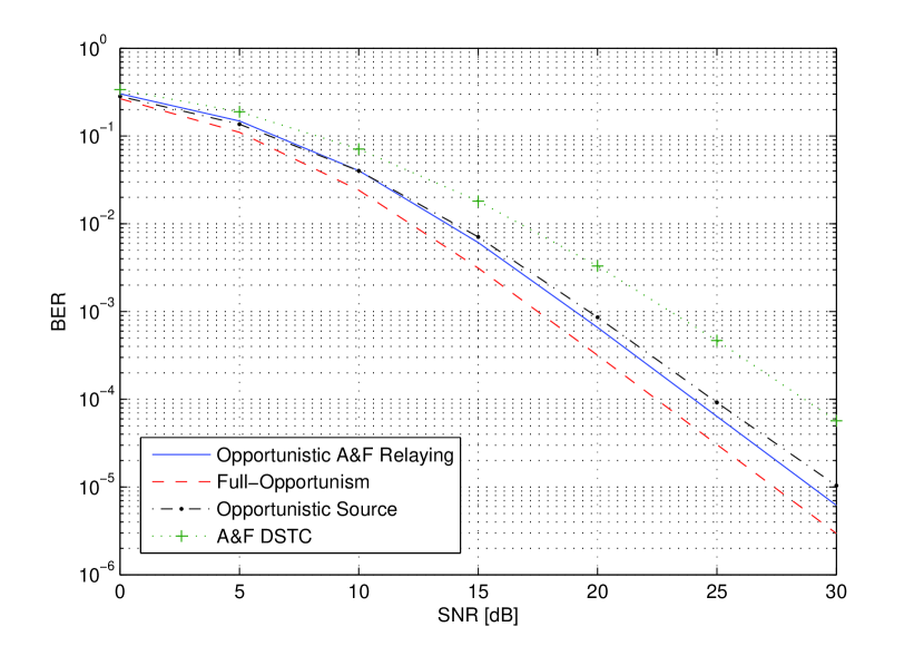
Figure 2: Performance comparison of A&F DSTC with multiple antenna source with the proposed opportunistic relaying schemes for a relay network with BPSK signals, $R=2$, $N_{s}=2$, $N_{d}=1$, and $T=4$.

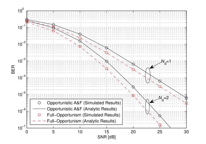
Figure 3: Performance comparison of analytical and simulated results of a relay network with BPSK signals, $R=2$, $N_{s}=2$, and $T=4$.

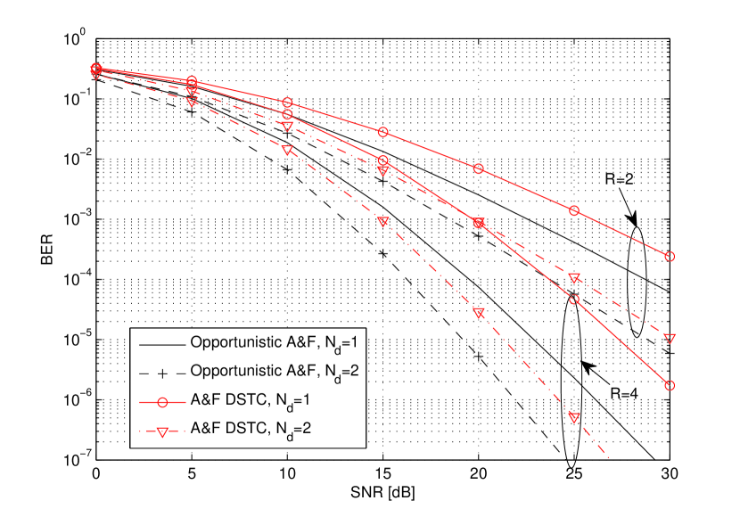
Figure 4: Performance comparison of A&F DSTC and opportunistic A&F relaying for a relay network for different values of relays and the destination antennas with BPSK signals, $N_{s}=1$, and $T=4$.

VI Simulation Results

In this section, the performance of distributed space-time codes are compared with opportunistic relaying schemes in A$\&$F mode presented in Section III. The signal symbols are modulated as BPSK. We fixed the total power consumed in the whole network as $P$ and use the equal power allocation, i.e, $P_{1}=P_{2}=\frac{P}{2}$. Assume that the relays and the destination have the same value of noise power, i.e., $\mathcal{N}_{1}=\mathcal{N}_{2}$, and all the links have unit-variance Rayleigh flat fading, i.e., $\sigma_{f_{r}}^{2}=\sigma_{g_{r}}^{2}=1$. Let $T=4$, and we use the orthogonal space-time code structure in (1) and (6). For the case of $N_{s}=2$, $R=2$, the matrices $\boldsymbol{A}_{1}$ and $\boldsymbol{A}_{2}$ used at the source and the matrices $\boldsymbol{C}_{1}$ and $\boldsymbol{C}_{2}$ used at the relays are as follows: $\boldsymbol{A}_{1}=\boldsymbol{C}_{1}=\boldsymbol{I}_{4}$, and

$$\boldsymbol{A}_{2}=\left[\begin{array}[]{cccc}0&-1&0&0\\ 1&0&0&0\\ 0&0&0&-1\\ 0&0&1&0\end{array}\right],{\,}\boldsymbol{C}_{2}=\left[\begin{array}[]{cccc}0&0&-1&0\\ 0&0&0&1\\ 1&0&0&0\\ 0&-1&0&0\end{array}\right]\!\!.$$ (87)

In Fig. 2, the BER performance of the A$\&$F DSTC is compared to the proposed opportunistic A$\&$F relaying schemes, when the number of available relays is 2. For A$\&$F DSTC, equal power allocation is used among the relays [11]. The opportunistic A$\&$F scheme is based on the power allocation presented in Subsection III-A, in which the distributed space-time code is applied across the source antennas in the first phase and the best relay is selected in the second phase of transmission. In another scheme, called full-opportunism, we use the power allocation derived in Subsection III-B, in which the CSI is available for the maximum SNR power allocation across the source’s antennas and the relays. The other scheme which is called opportunistic source and studied in Subsection III-C, uses the best antenna selection at the source and the distributed space-time code across the relays. One can observe from Fig. 2 that full-opportunism outperforms the opportunistic A$\&$F relaying scheme by more than 1.5 dB SNR at BER $10^{-4}$. Moreover, the opportunistic A$\&$F relaying and opportunistic source schemes achieve around 5 dB and 4 dB gain in SNR over A$\&$F DSTC at BER $10^{-4}$. Observing the curves behavior in high SNR, it can be seen that the diversity order of the system agrees with $R\min\{N_{s},N_{d}\}$.

Fig. 3 confirms that the analytical results attained in Section IV for finding the average SER for opportunistic A$\&$F relaying with space-time coded source and also full-opportunism scheme have the same performance as the simulation results. In Fig. 3, we consider a network with $R=2$ and $N_{s}=2$ and two values of $N_{d}\in\{1,2\}$. The analytical results are based on (IV-A) and (IV-B) for opportunistic A$\&$F relaying and full-opportunism, respectively. It is shown that full-opportunism outperforms opportunistic A$\&$F relaying around 1.5 dB gain in SNR at BER $10^{-5}$ for both cases of $N_{d}=1$ and $N_{d}=2$.

In Fig. 4, the performance of A$\&$F DSTC and opportunistic A$\&$F relaying systems are compared for two values of relay numbers $R=2,4$, when a single antenna is used at the source, i.e., $N_{s}=1$, and $N_{d}=1,2$. Since it is assumed $N_{s}=1$, opportunistic A$\&$F relaying and full-opportunism have the same performance. In addition, A$\&$F DSTC and opportunistic source schemes become equivalent. Observing the curves behavior at high SNR, it can be seen that the diversity order of the system becomes $R\min\{N_{s},N_{d}\}$. Furthermore, it can be seen that the performance of A$\&$F DSTC in low SNR conditions degrades as the number of relays increases due to the noise accumulation in the relays. For example, although A$\&$F DSTC system with $R=4$, $N_{s}=1$, and $N_{d}=1$ achieve the diversity gain of 4 in comparison to A$\&$F DSTC system with $R=2$, $N_{s}=1$, and $N_{d}=2$ with the diversity gain of 2, the former outperforms the latter about 2.5 dB at BER $10^{-2}$.

VII Conclusion

In this paper, we studied the problem of power allocation and coding for a wireless relay network where both the transmitter and receiver have several antennas, while each relay has one. Due to the high transmission rate, it is not assumed relays are able to decode, and thus, a distributed space-time scheme is used, where relays just do a simple operation on the received signal before forwarding it. The optimal transmit power from the source antennas and the relays in the sense of maximizing the SNR at the destination are derived for a A$\&$F wireless relay network with multiple antenna terminals. Based on the knowledge of CSI at the source and the relay, we have derive three transmission schemes. We analyzed the average SER performance of the A&F opportunistic relaying and full-opportunism systems with $M$-PSK and $M$-QAM signals. Simulations are in accordance with the analytic expressions. We also studied the asymptotic behavior of the proposed schemes and derived the closed-form SER formulas in the high SNR regime.

Appendix A Proof of Proposition 1

The average SNR at the destination can be obtained by dividing the average received signal power by the variance of the noise at the destination (approximation of $\mathbb{E}\{\text{SNR}_{\text{ins}}\}$ using Jensen’s inequality). Using (14), the average SNR can be written as

$$\text{SNR}=\frac{\tau(1-\tau)P^{2}\sigma_{f}^{2}\sigma_{g}^{2}}{\tau(\mathcal{N}_{2}\sigma_{f}^{2}-\mathcal{N}_{1}\sigma_{g}^{2})P+\mathcal{N}_{1}\sigma_{g}^{2}P+\mathcal{N}_{1}\mathcal{N}_{2}},$$ (88)

where we have assumed $\sigma_{f_{r}}^{2}=\sigma_{f}^{2}$ and $\sigma_{g_{r}}^{2}=\sigma_{g}^{2}$, for $r=1,\ldots,R$, and thus, $P_{2,r}=\frac{P_{2}}{R}$. First, we consider the case in which $\mathcal{N}_{2}\sigma_{f}^{2}\geq\mathcal{N}_{1}\sigma_{g}^{2}$. In this case, the optimum value of $\tau$ which maximizes (88), subject to the constraint $0<\tau<1$, is obtained as

$$\tau=\frac{\sqrt{1+\delta}-1}{\delta},$$ (89)

where

$$\delta=\frac{(\mathcal{N}_{2}\sigma_{f}^{2}-\mathcal{N}_{1}\sigma_{g}^{2})\,P}{\mathcal{N}_{1}\sigma_{g}^{2}P+\mathcal{N}_{1}\mathcal{N}_{2}}.$$ (90)

Similarly, when $\mathcal{N}_{2}\sigma_{f}^{2}<\mathcal{N}_{1}\sigma_{g}^{2}$, the optimum value of $\tau$, which maximizes SNR in (88), subject to constraint $0<\tau<1$, is also (89) and (90). Therefore, observing (89) and (90), the desired result in (41) is achieved.

Appendix B Proof of Proposition 2

Suppose $X=\|\boldsymbol{f}_{r}\|^{2}$ and $Y=\|\boldsymbol{g}_{r}\|^{2}$, where $X$ and $Y$ have gamma distribution [29, Eq. (5.14)] with mean of $\overline{X}_{\!r}$ and $\overline{Y}_{\!r}$, respectively. Therefore, the cumulative density function (CDF) of $\gamma_{r}=XY/(aY+b_{r})$ can be presented to be

$$\text{Pr}\{\gamma_{r}<\gamma\} =\text{Pr}\{XY/(aY+b_{r})<\gamma\}=\int_{0}^{\infty}\text{Pr}\left\{X<\frac{\gamma(ay+b_{r})}{y}\right\}p_{Y}(y)dy$$

$$=\int_{0}^{\infty}\!\!\left(1\!-\!\frac{\Gamma\left(N_{s},\frac{\gamma(ay+b_{r})}{y\overline{X}_{r}}\right)}{\Gamma(N_{s})}\right)\frac{y^{N_{d}-1}e^{-\frac{y}{\overline{Y}_{r}}}}{(N_{d}-1)!\,\overline{Y}_{r}^{N_{d}}}dy$$

$$=1\!-\!\int_{0}^{\infty}\!\frac{\Gamma\left(N_{s},\frac{\gamma(ay+b_{r})}{y\overline{X}_{r}}\right)}{\Gamma(N_{s})}\frac{y^{N_{d}-1}e^{-\frac{y}{\overline{Y}_{r}}}}{(N_{d}-1)!\,\overline{Y}_{r}^{N_{d}}}dy,$$ (91)

where we have used [33, Eq. (3.324)] for the third equality, $\Gamma(\alpha,x)$ is the incomplete gamma function of order $\alpha$ [34, Eq. (8.350)], and $p_{Y}(y)=\frac{y^{N_{d}-1}}{(N_{d}-1)!\overline{\gamma}_{r}^{N_{d}}}e^{-\frac{y}{\overline{Y}_{r}}}$ [29, Eq. (5.14)]. Then, using (B), $\Gamma(N_{s})=(N_{s}-1)!$, and $\frac{-d\,{\Gamma}(\alpha,x)}{dx}=x^{\alpha-1}e^{-x}$ [33, Eq. (8.356)], the PDF of $\gamma_{r}$ can be written as

$$p_{r}(\gamma) =\frac{\overline{X}_{\!r}^{\,-N_{s}}\gamma^{N_{s}-1}e^{-\frac{a\gamma}{\overline{X}_{\!r}}}}{\overline{Y}_{\!r}^{N_{d}}(N_{d}-1)!\,(N_{s}-1)!}\int_{0}^{\infty}y^{N_{d}-N_{s}-1}(ay+b_{r})^{N_{s}}e^{-\left(\frac{b_{r}\gamma}{\overline{X}_{\!r}y}+\frac{y}{\overline{Y}_{\!r}}\right)}dy$$

$$=\left(\frac{b_{r}}{\overline{X}_{\!r}}\right)^{\!\!N_{s}}\!\!\frac{\gamma^{N_{s}-1}e^{-\frac{a\gamma}{\overline{X}_{\!r}}}}{\overline{Y}_{\!r}^{N_{d}}(N_{d}-1)!\,(N_{s}-1)!}\sum_{k=0}^{N_{s}}{N_{s}\choose k}\int_{0}^{\infty}y^{N_{d}-N_{s}-1}\left(\frac{ay}{b_{r}}\right)^{\!\!k}e^{-\left(\frac{b_{r}\gamma}{\overline{X}_{\!r}y}+\frac{y}{\overline{Y}_{\!r}}\right)}dy,$$ (92)

where we have used binomial theorem [32, Eq. (2.36)] in the second equality. Thus, the PDF of $\gamma_{r}$ can be found by solving the integral in (B) using [33, Eq. (3.471)], yielding (43).

Appendix C Proof of Proposition 3

Suppose $X=\displaystyle\max_{n\in\{1,\ldots,N_{s}\}}|f_{n,r}|^{2}$ and $Y=\|\boldsymbol{g}_{r}\|^{2}$ where $Y$ has gamma distribution [29, Eq. (5.14)] with mean of $\overline{Y}_{\!r}$. Therefore, the cumulative density function (CDF) of $\zeta_{r}=XY/(\alpha Y+\beta_{r})$ can be presented to be

$$\text{Pr}\{\zeta_{r}<\zeta\} =\text{Pr}\{XY/(\alpha Y+\beta_{r})<\zeta\}=\int_{0}^{\infty}\text{Pr}\left\{X<\frac{\zeta(\alpha y+\beta_{r})}{y}\right\}p_{Y}(y)dy$$

$$=\int_{0}^{\infty}\text{Pr}\{|f_{1,r}|^{2}<\frac{\zeta(\alpha y+\beta_{r})}{y},\ldots,|f_{N_{s},r}|^{2}<\frac{\zeta(\alpha y+\beta_{r})}{y}\}p_{Y}(y)dy$$

$$=\int_{0}^{\infty}\prod_{n=1}^{N_{s}}\text{Pr}\left\{|f_{n,r}|^{2}<\frac{\zeta(\alpha y+\beta_{r})}{y}\right\}p_{Y}(y)dy$$

$$=\int_{0}^{\infty}\left(1-e^{-\frac{\zeta(\alpha y+\beta_{r})}{y\sigma_{f_{r}}^{2}}}\right)^{N_{s}}\frac{y^{N_{d}-1}}{(N_{d}-1)!\,\overline{Y}_{r}^{N_{d}}}e^{-\frac{y}{\overline{Y}_{r}}}dy$$

$$=\sum_{k=0}^{N_{s}}{N_{s}\choose k}\int_{0}^{\infty}e^{-\frac{\zeta(\alpha y+\beta_{r})k}{y\sigma_{f_{r}}^{2}}}\frac{(-1)^{k}y^{N_{d}-1}}{(N_{d}-1)!\,\overline{Y}_{r}^{N_{d}}}e^{-\frac{y}{\overline{Y}_{r}}}dy.$$ (93)

Then, the PDF of $\zeta_{r}$ can be written as

$$p_{\zeta_{r}}(\zeta)=\frac{d}{d\zeta}\text{Pr}\{\zeta_{r}<\zeta\}= \sum_{k=1}^{N_{s}}{N_{s}\choose k}\int_{0}^{\infty}e^{-\frac{\zeta(\alpha y+\beta_{r})k}{y\sigma_{f_{r}}^{2}}}\frac{(-1)^{k+1}k\,\alpha\,y^{N_{d}-1}}{(N_{d}-1)!\,\overline{Y}_{r}^{N_{d}}\sigma_{f_{r}}^{2}}e^{-\frac{y}{\overline{Y}_{r}}}dy$$

$$+\sum_{k=1}^{N_{s}}{N_{s}\choose k}\int_{0}^{\infty}e^{-\frac{\zeta(\alpha y+\beta_{r})k}{y\sigma_{f_{r}}^{2}}}\frac{(-1)^{k+1}k\,\beta_{r}\,y^{N_{d}-2}}{(N_{d}-1)!\,\overline{Y}_{r}^{N_{d}}\sigma_{f_{r}}^{2}}e^{-\frac{y}{\overline{Y}_{r}}}dy,$$ (94)

and using [33, Eq. (3.471)], the PDF of $\zeta_{r}$ yields to (3).

Appendix D Proof of Lemma 3

For finding the value of $p_{\zeta_{r}}(\zeta)$ and its derivatives around zero, we use the fifth equation of (C) to write

$$p_{\zeta_{r}}(\zeta)\!=\!\frac{d}{d\zeta}\text{Pr}\{\zeta_{r}<\zeta\}\!=\!\int_{0}^{\infty}\!\!\!N_{s}\!\left(1\!-\!e^{-\frac{\zeta(\alpha y+\beta_{r})}{y\sigma_{f_{r}}^{2}}}\right)^{\!N_{s}-1}\!e^{-\frac{\zeta(\alpha y+\beta_{r})}{y\sigma_{f_{r}}^{2}}}\frac{(\alpha y+\beta_{r})y^{N_{d}-2}}{\sigma_{f_{r}}^{2}(N_{d}-1)!\,\overline{Y}_{r}^{N_{d}}}e^{-\frac{y}{\overline{Y}_{r}}}dy.$$ (95)

Therefore, it follows from (C) that $p_{\zeta_{r}}\!(0)=0$. Moreover, from (C), it can be seen that $\frac{\partial^{n}p_{\zeta_{r}}}{\partial\zeta^{n}}(0)=0$, for $n=1,\ldots,N_{s}-2$, and $\frac{\partial^{N_{s}-1}p_{\zeta_{r}}}{\partial\zeta^{N_{s}-1}}(0)$ can be calculated as

$$\frac{\partial^{N_{s}-1}p_{\zeta_{r}}}{\partial\zeta^{N_{s}-1}}(0)=\lim_{\zeta\rightarrow 0}\int_{0}^{\infty}N_{s}!\left(\frac{\alpha y+\beta_{r}}{y\sigma_{f_{r}}^{2}}\right)^{\!\!N_{s}}e^{-\frac{N_{s}\zeta(\alpha y+\beta_{r})}{y\sigma_{f_{r}}^{2}}}\frac{y^{N_{d}-1}}{(N_{d}-1)!\,\overline{Y}_{r}^{N_{d}}}e^{-\frac{y}{\overline{Y}_{r}}}dy$$

$$=\lim_{\zeta\rightarrow 0}\sum_{k=1}^{N_{s}}\!\frac{\alpha^{N_{s}-k}\beta_{r}^{k}N_{s}!{N_{s}\choose k}e^{-\frac{N_{s}\alpha\zeta}{\sigma_{f_{r}}^{2}}}}{(N_{d}\!\!-\!\!1)!\overline{Y}_{r}^{N_{d}}}\int_{0}^{\infty}e^{-\frac{N_{s}\zeta\beta_{r}}{y\sigma_{f_{r}}^{2}}-\frac{y}{\overline{Y}_{r}}}y^{N_{d}-k-1}dy$$

$$=\lim_{\zeta\rightarrow 0}\sum_{k=1}^{N_{s}}\!\frac{2\alpha^{N_{s}-k}\beta_{r}^{k}N_{s}!{N_{s}\choose k}e^{-\frac{N_{s}\alpha\zeta}{\sigma_{f_{r}}^{2}}}}{(N_{d}\!\!-\!\!1)!\overline{Y}_{r}^{N_{d}}}\left(\!\frac{\beta_{r}k\overline{Y}_{\!r}\zeta}{\sigma_{f_{r}}^{2}}\!\right)^{\!\!\!\frac{N_{d}-k}{2}}\!\!\!\!\!K_{N_{d}-k}\!\!\left(\!2\sqrt{\!\frac{k\beta_{r}\zeta}{\sigma_{f_{r}}^{2}\!\overline{Y}_{\!r}}}\right).$$ (96)

Using the fact that $K_{\nu}(x)\approx\frac{1}{2}\Gamma(\nu)\left(\frac{x}{2}\right)^{-\nu},\,\nu\neq 0$ [34, Eq. (9.6.9)], as $x\rightarrow 0$, $\frac{\partial^{N_{s}-1}p_{\zeta_{r}}}{\partial\zeta^{N_{s}-1}}(0)$ in (D) can be approximated as

$$\frac{\partial^{N_{s}-1}p_{\zeta_{r}}}{\partial\zeta^{N_{s}-1}}(0)\! =\lim_{\zeta\rightarrow 0}\sum_{k=1}^{N_{s}}\!\frac{\alpha^{N_{s}-k}\beta_{r}^{k}N_{s}!{N_{s}\choose k}(N_{d}\!-k\!-\!\!1)!\,e^{-\frac{N_{s}\alpha\zeta}{\sigma_{f_{r}}^{2}}}}{(N_{d}\!-\!1)!\overline{Y}_{r}^{\,-k}}$$

$$=\sum_{k=1}^{N_{s}}\!\frac{\alpha^{N_{s}-k}\beta_{r}^{k}N_{s}!{N_{s}\choose k}(N_{d}\!-k\!-\!1)!}{(N_{d}\!-\!1)!\overline{Y}_{r}^{\,-k}},$$ (97)

which completes the proof.

References

- [1] A. Sendonaris, E. Erkip, and B. Aazhang, “User cooperation diversity. Part I. System description,” IEEE Trans. Commun., vol. 51, no. 11, pp. 1927–1938, Nov. 2003.
- [2] A. Sendonaris, E. Erkip, and B. Aazhang, “User cooperation diversity. Part II. Implementation aspects and performance analysis,” IEEE Trans. Commun., vol. 51, pp. 1939–1948, Nov. 2003.
- [3] J. N. Laneman and G. Wornell, “Energy-efficient antenna sharing and relaying for wireless networks,” in Proc. Wireless Communications Networking Conf., (Chicago, IL), pp. 7–12, Sep. 2000.
- [4] J. N. Laneman and G. Wornell, “Distributed space-time coded protocols for exploiting cooperative diversity in wireless networks,” in IEEE GLOBECOM 2002, vol. 1, (Taipei, Taiwan, R.O.C.), pp. 77–81, Nov. 2002.
- [5] R. U. Nabar, H. Bölcskei, and F. W. Kneubuhler, “Fading relay channels: Performance limits and space-time signal design,” IEEE J. Sel. Areas Commun., vol. 22, no. 6, pp. 1099–1109, Aug. 2004.
- [6] Y. Hua, Y. Mei, and Y. Chang, “Wireless antennas-making wireless communications perform like wireline communications,” in IEEE AP-S Topical Conf. on Wireless Comm. Tech., (Honolulu, Hawaii), Oct. 2003.
- [7] Y. Jing and B. Hassibi, “Distributed space-time coding in wireless relay networks,” IEEE Trans. Wireless Commun., vol. 5, no. 12, pp. 3524–3536, Dec. 2006.
- [8] Y. Jing and H. Jafarkhani, “Using orthogonal and quasi-orthogonal designs in wireless relay networks,” IEEE Trans. Info. Theory, vol. 53, no. 11, pp. 4106–4118, Nov. 2007.
- [9] B. Maham, A. Hjørungnes, and G. Abreu, “Distributed GABBA space-time codes in amplify-and-forward relay networks,” IEEE Trans. Wireless Commun., vol. 8, no. 4, pp. 2036–2045, Apr. 2009.
- [10] G. S. Rajan and B. S. Rajan, “Distributed space-time codes for cooperative networks with partial CSI,” in Proc. IEEE Wireless Communications and Networking Conference (WCNC), (Hong Kong, China), pp. 902–906, March 2007.
- [11] Y. Jing and B. Hassibi, “Cooperative diversity in wireless relay networks with multiple-antenna nodes,” in IEEE Int. Symp. Inform. Theory, (Adelaide, Australia), 2005.
- [12] S. Peters and R. W. Heath, “Selection cooperation in multi-source cooperative networks,” IEEE Signal Processing Letters, vol. 15, pp. 421–424, Jan. 2008.
- [13] F. Oggier and B. Hassibi, “An algebraic coding scheme for wireless relay networks with multiple-antenna nodes,” IEEE Trans. Signal Process., vol. 56, no. 7, pp. 2957–2966, Jul. 2008.
- [14] Y.-W. Hong, W.-J. Huang, F.-H. Chiu, and C.-C. J. Kuo, “Cooperative communications in resource-constrained wireless networks,” IEEE Signal Processing Magazine, vol. 24, pp. 47–57, May 2007.
- [15] B. Maham and A. Hjørungnes, “Minimum power allocation in SER constrained amplify-and-forward cooperation,” in Proc. IEEE Vehicular Technology Conference (VTC 2008-Spring), (Singapore), pp. 2431–2435, May 2008.
- [16] M. Chen, S. Serbetli, and A. Yener, “Distributed power allocation strategies for parallel relay networks,” IEEE Trans. Wireless Commun., vol. 7, no. 2, pp. 552–561, Feb. 2008.
- [17] A. Host-Madsen and J. Zhang, “Capacity bounds and power allocation for wireless relay channels,” IEEE Trans. Inform. Theory, vol. 51, no. 6, pp. 2020–2040, Jun. 2005.
- [18] D. R. Brown, “Energy conserving routing in wireless adhoc networks,” in Proc. Asilomar Conf. Signals, Syst. Computers, (Monterey, CA, USA), Nov. 2004.
- [19] A. Reznik, S. R. Kulkarni, and S. Verdú, “Degraded Gaussian multirelay channel: Capacity and optimal power allocation,” IEEE Trans. Inform. Theory, vol. 50, no. 12, pp. 3037–3046, Dec. 2004.
- [20] M. O. Hansa and M.-S. Alouini, “Optimal power allocation for relayed transmissions over Rayleigh-fading channels,” IEEE Trans. Wireless Commun., vol. 3, no. 6, pp. 1999–2004, Nov. 2004.
- [21] M. Dohler, A. Gkelias, and H. Aghvami, “Resource allocation for FDMA-based regenerative multihop links,” IEEE Trans. Wireless Commun., vol. 3, no. 6, pp. 1989–1993, Nov. 2004.
- [22] J. Luo, R. S. Blum, L. J. Cimini, L. J. Greenstein, and A. M. Haimovich, “Link-failure probabilities for practical cooperative relay networks,” in Proc. IEEE 61st Veh. Technol. Conf., Spring, pp. 1489–1493, May 2005.
- [23] Z. Lin and E. Erkip, “Relay search algorithms for coded cooperative systems,” in Proc. IEEE Global Telecommun. Conf., pp. 1314–1319, Nov. 2005.
- [24] H. Zheng, Y. Zhu, C. Shen, and X. Wang, “On the effectiveness of cooperative diversity in ad hoc networks: A MAC layer study,” in IEEE Int. Conf. Acoustics, Speech, Signal Processing, pp. 509–512, Mar. 2005.
- [25] A. Bletsas, A. Khisti, D. P. Reed, and A. Lippman, “A simple cooperative method based on network path selection,” IEEE Journal on Selected Areas in Communications, vol. 24, no. 3, pp. 659–672, Mar. 2006.
- [26] A. Bletsas, H. Shin, and M. Win, “Outage optimality of amplify-and-forward opportunistic relaying,” IEEE Comm. Letters, vol. 11, pp. 261–263, Mar. 2007.
- [27] Y. Zhao, R. Adve, and T. J. Lim, “Symbol error rate of selection amplify-and-forward relay systems,” IEEE Comm. Letters, vol. 10, no. 11, pp. 757–759, Nov. 2006.
- [28] Z. Wang and G. Giannakis, “A simple and general parameterization quantifying performance in fading channels,” IEEE Trans. Commun., vol. 51, no. 8, pp. 1389–1398, Aug. 2003.
- [29] M. K. Simon and M.-S. Alouini, Digital Communication over Fading Channels: A Unified Approach to Performance Analysis. New York, USA: Wiley, 2000.
- [30] B. Maham and A. Hjørungnes, “Orthogonal code design for MIMO amplify-and-forward cooperative networks,” in Proc. IEEE Information Theory Workshop (ITW’07), (Cairo, Egypt), Jan. 2010.
- [31] R. Horn and C. Johnson, Matrix Analysis. Cambridge, UK: Cambridge Academic Press, 1985.
- [32] A. Leon-Garcia, Probability and Random Processes for Electrical Engineering. Massachusetts, USA: Addison-Wesley Publishing Company, 1994.
- [33] I. S. Gradshteyn and I. M. Ryzhik, Table of Integrals, Series, and Products. San Diego, USA: Academic, 1996.
- [34] M. Abramowitz and I. A. Stegun, Handbook of Mathematical Functions. New York, USA: Dover Publications, 1972.
- [35] H. Jafarkhani, Space-Time Coding Theory and Practice. Cambridge, UK: Cambridge Academic Press, 2005.