Relaxation of protostellar accretion shocks using the smoothed particle hydrodynamics

Abstract

It is believed that protostellar accretion disks to be formed from nearly ballistic infall of the molecular matters in rotating core collapse. Collisions of these infalling matters lead to formation of strong supersonic shocks, which if they cool rapidly, result in accumulation of that material in a thin structure in the equatorial plane. Here, we investigate the relaxation time of the protostellar accretion post-shock gas using the smoothed particle hydrodynamics (SPH). For this purpose, a one-dimensional head-on collision of two molecular sheets is considered, and the time evolution of the temperature and density of the post-shock region simulated. The results show that in strong supersonic shocks, the temperature of the post-shock gas quickly increases proportional to square of the Mach number, and then gradually decreases according to the cooling processes. Using a suitable cooling function shows that in appropriate time-scale, the center of the collision, which is at the equatorial plane of the core, is converted to a thin dense molecular disk, together with atomic and ionized gases around it. This structure for accretion disks may justify the suitable conditions for grain growth and formation of proto-planetary entities.

1 Introduction

In the general picture, the gravitational unstable molecular cloud cores collapse and form the protostars, accretion disks, and outflows. The first model of a spherical symmetric accretion which flow towards a central object was made by Bondi (1952). Years later, Ulrich (1976) modified the Bondi’s idea by assuming all fluid particles have a certain angular momentum with negligible pressure forces at the border of the cloud, so that the collapse problem analyzed using ballistic trajectories. Since then, many generalizations of the core collapse have been made (e.g., Shu 1977, Terebey, Shu & Cassen 1984, Foster & Chevalier 1993, Galli & Shu 1993, Henriksen, André & Bontemps 1997, Fatuzzo, Adams & Myers 2004, Mendoza, Tejeda & Nagel 2009, Bate 2010, Nejad-Asghar 2010). As a result of rotating collapse, the collisions at the equatorial plane, between the infalling matters coming from the northern hemisphere and those coming from the southern one, cause the formation of strong supersonic shocks. If the shocked gas cools rapidly, the result is that material accumulates in a thin structure in the equatorial plane, i.e., accretion disk (Hartmann 2009).

Observations have revealed not only the existence of the circumstellar disks around the protostars (e.g., Watson et al. 2007, Akeson 2008, Quanz et al. 2010), but also the occurrence of jets and outflows (e.g., Hirth, Mundt & Solf 1997, Wu et al. 2004, Dunham et al. 2010). The outflows and jets are ubiquitous together with accretion disks through the collapsing molecular cloud cores (e.g., Furuya, Cesaroni & Shinnaga 2011). We cannot directly observe the newborn or very young accretion disks and jets because their formation places are embedded in a dense infalling envelope. On the other words, observations cannot directly determine the real structure and formation history of accretion disks and outflows. Therefore, theoretical approach and simulations are necessary to investigate the formation and evolution of them (e.g., Walch et al. 2009, Machida, Inutsuka & Matsumoto 2010, Ciardi & Hennebelle 2010, Nejad-Asghar 2011). Clearly, consideration of jets and magnetic fields can affect on formation and evolution of accretion disks (e.g., Hujeirat 1998, Hujeirat et al. 2003, Machida, Inutsuka & Matsumoto 2007), but in this study, we turn our attention to the phase after formation of of central protostar, and for simplicity neglect the effect of jets and outflows on protostellar accretion shocks. In addition to physical evolution of circumstellar disks, the chemical evolution from the core to the disk phase is also important (e.g., Ceccarelli, Hollenbach & Tielens 1996, Rodgers & Charnley 2003, Garrod & Herbst 2006, Garrod, Weaver & Herbst 2008, Visser et al. 2009). Here, we assume that all effects of chemical evolution of shocked gas are simplified through the appropriate net cooling function.

Interstellar shocks cover a wide range of parameters: velocities of $1-10^{4}\mathrm{km.s^{-1}}$, pre-shock densities of $10^{-2}-10^{7}\mathrm{cm^{-3}}$, and post-shock temperatures of $10^{2}-10^{9}\mathrm{K}$. The strength of a shock is indicated by the Mach number which can range up to $\sim 10^{3}$, for larger than laboratory shocks (McKee & Hollenbach 1980). For an adiabatic strong shock, the jump in density is limited to a factor of four (for a ratio of specific heats $\gamma=5/3$), while the temperature of post-shock gas can be increased proportional to the square of Mach number (e.g., Dyson & Williams 1997). As mentioned above, the high velocity of infalling matters at the equatorial plane of a rotating core collapse, leads to strong supersonic collisions with great Mach numbers. The high temperature of the post-shock gas causes the molecule dissociation and the atom ionization. Neufeld & Hollenbach (1994) examined the physical and chemical processes of high-density accretion shocks which associated with the supersonic infall of material during the collapse of a molecular cloud core to form a protostar. Since the rotation and magnetic fields cause the deflection of infalling matters from the protostar so that a shocked disk gas is formed, here we study the physical and chemical evolutions of these shocked circumstellar disks for understanding the formation of structure and substructures through them.

As a general aspect of star formation, we expect that cooling (as a result of chemical and physical changes) of the protostellar accretion shocked gas at the equatorial plane of collapsing core leads to supply the suitable conditions for grain growth and formation of proto-planetary entities. The goal of this paper is to investigate this expectation. For this purpose, the jump shock (J-shock) structure and the cooling time-scale of post-shock gas are presented in section 2. In section 3, we use the SPH methodology to investigate the time evolution of the strong supersonic shocks. Finally, section 4 is devoted to summary and conclusions.

2 J-shock structure

For simplicity, the shock is assumed planar and steady in which the deceleration is negligible and there is no thermal instability in the cooling layer. The jump conditions of this shock (J-shock) relate the quantities at an arbitrary point behind the shock front to those ahead of it. Conservation of mass, momentum, and energy across the shock front is given by Rankine-Hugoniot conditions (e.g., Dyson & Williams 1997)

$$\rho_{1}v_{1}=\rho_{2}v_{2}$$ (1)

$$\rho_{1}v_{1}^{2}+\mathcal{K}_{1}\rho_{1}T_{1}=\rho_{2}v_{2}^{2}+\mathcal{K}_{2}\rho_{2}T_{2}$$ (2)

$$\frac{1}{2}v_{1}^{2}+\frac{\gamma_{1}}{\gamma_{1}-1}\mathcal{K}_{1}T_{1}=\frac{1}{2}v_{2}^{2}+\frac{\gamma_{2}}{\gamma_{2}-1}\mathcal{K}_{2}T_{2}+Q$$ (3)

where $\gamma$ is the ratio of specific heats, $Q$ is the energy lost per unit mass during the shock process, and the equation of state is applied as $p=(k/\mu m_{H})\rho T=\mathcal{K}\rho T$. The jump conditions (1)-(3) enable one to solve the J-shock structure.

We would be interested to consider the collision of two gas sheets with velocities $v_{0}$ in the rest frame of laboratory. In this reference frame, the post-shock will be at rest and the pre-shock velocity is given by $v_{1}=v_{0}+v_{2}$, where $v_{2}$ is the shock front velocity. Defining the pre-shock sound speed as $c\equiv\sqrt{\mathcal{K}_{1}T_{1}}$ and Mach number as $M_{0}\equiv v_{0}/c$, the equations (1)-(3) lead to

$$\mathcal{T}=\frac{1}{\mathcal{R}}+\frac{M_{0}^{2}}{\mathcal{R}-1},$$ (4)

$$\mathcal{T}=\frac{\gamma_{1}}{\gamma_{2}}\frac{\gamma_{2}-1}{\gamma_{1}-1}+\frac{\gamma_{2}-1}{2\gamma_{2}}\frac{\mathcal{R}+1}{\mathcal{R}-1}M_{0}^{2}-\frac{(\gamma_{2}-1)Q}{\gamma_{2}c^{2}},$$ (5)

where $\mathcal{T}\equiv\mathcal{K}_{2}T_{2}/\mathcal{K}_{1}T_{1}$ and $\mathcal{R}\equiv\rho_{2}/\rho_{1}$ are the relative temperature and density of the post-shock gas, respectively. Eliminating $\mathcal{T}$ between the equations (4) and (5), gives the square equation

$$\mathcal{R}^{2}+A_{1}\mathcal{R}+A_{2}=0,$$ (6)

with coefficients as follows

$$A_{1} = -\frac{\frac{\gamma_{2}+1}{\gamma_{2}-1}M_{0}^{2}+\frac{2\gamma_{1}}{\gamma_{1}-1}+\frac{2\gamma_{2}}{\gamma_{2}-1}-\frac{2Q}{c^{2}}}{M_{0}^{2}+\frac{2\gamma_{1}}{\gamma_{1}-1}-\frac{2Q}{c^{2}}}$$

$$A_{2} = \frac{\frac{2\gamma_{2}}{\gamma_{2}-1}}{M_{0}^{2}+\frac{2\gamma_{1}}{\gamma_{1}-1}-\frac{2Q}{c^{2}}}.$$

In the general case, the solution of equation (6) can directly be found according to four parameters $\gamma_{1}$, $\gamma_{2}$, $Q$ and $M_{0}$; then the relative temperature $\mathcal{T}$ is obtained via equations (4) or (5). The adiabatic shock is a special case with $Q=0$, which in the strong supersonic collision ($M_{0}\rightarrow\infty$), the equation (6) leads to $\mathcal{R}=4$ with assumption of $\gamma_{2}=5/3$. In this case, the relative temperature is limitless as $\mathcal{T}\approx M_{0}^{2}/3$. In fact, this temperature is the maximum allowed value in a shock process, which is $T_{2}^{max}=3.86\mu_{2}\times 10^{5}v_{07}^{2}\mathrm{K}$ where $v_{07}\equiv v_{0}/100\mathrm{km.s^{-1}}$ (e.g., Hollenbach & McKee 1979). The most important parameter in the strong supersonic shocks ($M_{0}>>1$) is the energy lost per unit mass during the shock process, $Q=(n_{2}\Lambda/\mu_{2}m_{H})t_{dur}$, where $\Lambda$ ($\mathrm{erg.cm^{3}.s^{-1}}$) is the cooling function at the post-shock region with density $n_{2}$, and $t_{dur}$ is the duration time of the post-shock gas. Accurate determination of the cooling time-scale requires specifying the elemental abundance of the post-shock region, but a simple estimate can be obtained using $t_{cool}\approx kT_{2}/(n_{2}\Lambda)$. Eliminating the $n_{2}\Lambda$, we approximately have $Q/c^{2}\approx T(t_{dur}/t_{cool})$. If the post-shock gas cools rapidly (i.e., $t_{cool}<<t_{dur}$), its temperature cannot be grater than the molecular dissociation energy, while in slow cooling rate (i.e., $t_{cool}>>t_{dur}$), the temperature may even be grater than $10^{4}\mathrm{K}$ causing the atomic ionization process.

The cooling mechanisms take into account many different processes that dominate in different ranges of temperature. We apply the cooling function as outlined in the Figure 1 of Heitsch, Hartmann & Burkert (2008) in which they used a combination of the rates quoted by Dalgarno and McCray (1972) and Wolfire et al. (1995) for $T<10^{4}\mathrm{K}$, and the tabulated curves of Sutherland and Dopita (1993) for $T>10^{4}\mathrm{K}$. We can express the logarithm of cooling function as a piecewise linear function of the temperature logarithm as follows

$$\Lambda=\Lambda_{0}\left(\frac{T}{T_{0}}\right)^{\beta},$$ (7)

where $\Lambda_{0}$, $T_{0}$ and $\beta$ are given in Table 1 for ionization degree $x_{i}=0.1$ and metallicities corresponding to the solar neighborhood. In this way, the cooling time-scale can be expressed in a piecewise form as

$$t_{cool}\approx\frac{kT_{0}^{\beta}}{n_{2}\Lambda_{0}}T^{1-\beta},$$ (8)

which is shown in Fig. 1 for $n_{2}\sim 10^{4}\mathrm{cm^{-3}}$.

Table 1: Parameters for the piecewise linear expression of the cooling function, $\Lambda=\Lambda_{0}(T/T_{0})^{\beta}$, with ionization degree $x_{i}=0.1$ and with metallicities corresponding to the solar neighborhood.

$\log T$	$\Lambda_{0}(\mathrm{erg.cm^{3}.s^{-1}})$	$T_{0}(\mathrm{K})$	$\beta$
$1.00\rightarrow 1.75$	$1.74\times 10^{-28}$	$10$	$3.59$
$1.75\rightarrow 3.75$	$8.51\times 10^{-26}$	$56$	$0.47$
$3.75\rightarrow 4.21$	$7.41\times 10^{-25}$	$5623$	$5.11$
$4.21\rightarrow 4.47$	$1.66\times 10^{-22}$	$16218$	$-0.42$
$4.47\rightarrow 4.94$	$1.29\times 10^{-22}$	$29512$	$1.89$
$4.94\rightarrow 5.35$	$1.00\times 10^{-21}$	$87096$	$0.17$
$5.35\rightarrow 5.68$	$1.17\times 10^{-21}$	$223872$	$-2.36$
$5.68\rightarrow 6.17$	$1.95\times 10^{-22}$	$478630$	$-0.51$
$6.17\rightarrow 6.88$	$1.10\times 10^{-22}$	$1479109$	$-0.87$
$6.88\rightarrow 7.38$	$2.63\times 10^{-23}$	$7585778$	$-0.26$
$7.38\rightarrow 8.00$	$1.95\times 10^{-23}$	$23988340$	$0.21$

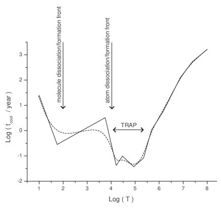
Figure 1: The cooling time-scale as expressed in a piecewise linear form for ionization degree $x_{i}=0.1$ and metallicities corresponding to the solar neighborhood. The dotted curve is the B-spline fit to this piecewise linear expression. The temperatures in which the molecules and atoms dissociate/form are depicted as arrows, and the minimum value of cooling time-scale is nominated as trap.

When the strong shocking molecular gases proceed, at the first time, the temperature increases near $T_{2}^{max}$ so that the molecules will be dissociated and the atoms may be ionized. In the ionized region, there is a trap in which $t_{cool}$ reaches to its minimum value so that the plasma gas cools rapidly to recombine the electrons and nucleons. Recombination becomes important when the post-shock plasma cools to $10^{4}\mathrm{K}$; a typical $H$ atomic recombination time-scale is approximately $t_{rec}\approx 1/n_{e}\alpha_{rec}\approx 10^{5}/n_{e}(\mathrm{cm^{-3}})\mathrm{yr}$, where $\alpha_{rec}$ is the total recombination coefficient and $n_{e}$ is the number density of electron (Osterbrock & Ferland 2006). If the process of cooling mode continues, the atomic post-shock gas will approach to the molecular gas. The $H_{2}$ molecule cannot form in the gas phase because it is not lonely able to radiate away the excess energy of formation. The grains, which have been survived in the shock process, can thus transfer this extra energy of $H_{2}$ formation to their phonons (Hollenbach & Salpeter 1971). Although, the details of this mechanism are rather complex, a simple estimation of $H_{2}$ formation time-scale is $t_{mol}\approx 1/n_{H}k_{m}\approx 10^{9}/n_{H}^{3}(\mathrm{cm^{-3}})\mathrm{yr}$, where $k_{m}\approx 3\times 10^{-17}n_{H}(n_{H}+2n_{H_{2}})$ $\mathrm{cm^{3}.s^{-1}}$ is the hydrogen molecule formation rate on the grain surfaces and $n_{H}$ is the hydrogen atomic number density (Lequeux 2005). For a typical J-shock structure of a protostellar accretion shocks, with $n_{e}\approx n_{H}\approx 10^{4}\mathrm{cm^{-3}}$, we have $t_{rec}\approx 10\mathrm{yr}$ and $t_{mol}\approx 10^{-3}\mathrm{yr}$, thus the recombination occurs slowly while the molecule formation occurs very fast. Although, we find some insights for J-shock structure and its relaxation process, but the shock process is rather a complex non-equilibrium thermal and chemical mechanism. Thus, in the next section, we use the SPH simulation to study the time evolution of processes in the strong shocking molecular gases.

3 Investigation by SPH

We consider the head-on collisions of two molecular gas sheets. An initial negative velocity is given to the particles with a positive $x$-coordinate, and a velocity in the opposite direction to those with a negative $x$-coordinate. Compositions of the sheets are assumed as global neutral which consists of a mixture of atomic and molecular hydrogen ($X\approx 0.75$), helium ($Y\approx 0.25$), and traces of CO and other rare molecules. The mean molecular weight is initially $1/\mu=X/2+Y/4\approx 0.4375$ for molecular case ($T<10^{2}\mathrm{K}$), and in the post-shock region for simplicity is assumed to be $1/\mu=X+Y/4\approx 0.8125$ for atomic case ($10^{2}\mathrm{K}<T<10^{4}\mathrm{K}$), and $1/\mu=2X+3Y/4\approx 1.6875$ for ionized case ($T>10^{4}\mathrm{K}$). The same procedure is followed for the ratio of specific heats: $\gamma=7/5$ for diatomic molecular gas and $\gamma=5/3$ for atomic and ionized cases. The chosen physical scales for length and time are $[l]=3.0\times 10^{14}\mathrm{cm}=20\mathrm{AU}$ and $[t]=3.0\times 10^{7}\mathrm{s}=1\mathrm{yr}$, respectively, so the velocity unit is approximately $100~{}\mathrm{km.s^{-1}}$. The gravitational constant is set $G=10^{-12}[l]^{3}.[t]^{-2}.[m]^{-1}$ for which the calculated mass unit is $[m]=4.5\times 10^{23}\mathrm{g}$. Consequently, the physical scales for density and energy are $[\rho]=1.6\times 10^{-20}\mathrm{g.cm^{-3}}=10^{4}\mathrm{H.cm^{-3}}$ and $[e]=4.5\times 10^{30}\mathrm{erg}$, respectively. Two equal one dimensional molecular sheets with extension $x=0.1[l]$ is considered, which have initial uniform density and temperature of $10^{4}\mathrm{cm^{-3}}$ and $\sim 10\mathrm{K}$, respectively.

The SPH method is well suited to address unbound astrophysical problems, especially the behavior of gases subjected to compression (Rosswog 2009). A worthy review of the SPH methodology and its applications can be found in Monaghan (2005). In this method, fluid is represented by $N$ discrete but extended/smoothed particles (i.e. Lagrangian sample points). The particles are overlapping, so that all the involved physical quantities can be treated as continuous functions both in space and time. Overlapping is represented by the kernel function, $W_{ab}\equiv W(\textbf{r}_{a}-\textbf{r}_{b},h_{ab})$, where $h_{ab}\equiv(h_{a}+h_{b})/2$ is the mean smoothing length of two particles $a$ and $b$. The density is estimated via usual summation over neighboring particles,

$$\rho_{a}=\sum_{b}m_{b}W_{ab},$$ (9)

the acceleration equation in the one-dimensional usual symmetric form is

$$\frac{dv_{a}}{dt}=-\sum_{b}m_{b}(\frac{p_{a}}{\rho_{a}^{2}}+\frac{p_{b}}{\rho_{b}^{2}}+\Pi_{ab})\frac{dW_{ab}}{dx_{a}},$$ (10)

and the SPH equivalent of the energy equation is

$$\frac{du_{a}}{dt}=\frac{1}{2}\sum_{b}m_{b}(\frac{p_{a}}{\rho_{a}^{2}}+\frac{p_{b}}{\rho_{b}^{2}}+\Pi_{ab})v_{ab}\frac{dW_{ab}}{dx_{a}}$$

$$-\frac{\Lambda_{0}}{(\mu_{a}m_{H})^{2}}\rho_{a}\left(\frac{T_{a}}{T_{0}}\right)^{\beta},$$ (11)

where $u_{a}=\frac{1}{\gamma_{a}-1}\mathcal{K}_{a}T_{a}$ is the thermal energy per unit mass, and $\Pi_{ab}$ is the artificial viscosity between particles $a$ and $b$

$$\Pi_{ab}=\cases{\frac{-\alpha^{*}v_{sig}\mu_{ab}^{*}+\beta^{*}\mu_{ab}^{*2}}{\bar{\rho}_{ab}},&if $\textbf{v}_{ab}.\textbf{r}_{ab}<0$,\cr 0,&otherwise,}$$ (12)

where $\textbf{v}_{ab}\equiv\textbf{v}_{a}-\textbf{v}_{b}$ and $\textbf{r}_{ab}\equiv\textbf{r}_{a}-\textbf{r}_{b}$ are relative velocity and the distance of particles, $\bar{\rho}_{ab}=\frac{1}{2}(\rho_{a}+\rho_{b})$ is an average density, $v_{sig}=(c_{a}+c_{b})/2$ is signal velocity where $c_{a}$ and $c_{b}$ are the sound speed of particles, and $\mu_{ab}^{*}$ is defined as its usual form

$$\mu_{ab}^{*}=\frac{\textbf{v}_{ab}\cdot\textbf{r}_{ab}}{h_{ab}}\frac{1}{r_{ab}^{2}/h_{ab}^{2}+\eta^{2}}$$ (13)

with $\eta\sim 0.1$.

To prevent unphysical solutions with inter-particle penetration and unwanted heating, we use $\alpha^{*}$ and $\beta^{*}$ in the form of variables with respect to time,

$$\frac{d\alpha^{*}_{a}}{dt}=-\frac{\alpha^{*}_{a}-\alpha_{\mathrm{min}}}{\tau_{a}}+z_{\alpha}\mathcal{S}_{a},$$ (14)

and

$$\frac{d\beta^{*}_{a}}{dt}=-\frac{\beta^{*}_{a}-\beta_{\mathrm{min}}}{\tau_{a}}+z_{\beta}\mathcal{S}_{a},$$ (15)

respectively, where $\mathcal{S}_{a}=\max(-\frac{dv_{a}}{dx_{a}},\frac{\dot{\rho}_{a}}{\rho_{a}}-\frac{\dot{h}_{a}}{h_{a}}-\frac{v_{\mathrm{sig}}}{r_{ab}},0)$ is the restricted source term, $\tau_{a}\equiv h_{a}/(\mathcal{C}v_{sig})$ with $0.1<\mathcal{C}<0.2$ is the decay time-scale, and the parameters $z_{\alpha}$ and $z_{\beta}$ are chosen to regulate the effect of source term so that the heat production and post-shock oscillations are controlled in the numerical simulations (Nejad-Asghar, Khesali & Soltani 2008). Here, we choose $\alpha_{min}=1$, $\beta_{min}=2$, $\mathcal{C}=0.2$, $z_{\alpha}=3$, and $z_{\beta}=0.01$ for the best smoothed results of simulations (see, e.g., Fig. 2). Clearly, comparison between numerical and analytical results in Fig. 2 verifies the accuracy and physical consistency of the employed numerical tool.

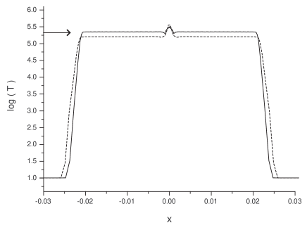
(a)

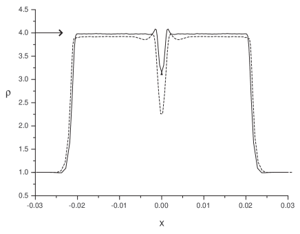
(b)

Figure 2: (a) Temperature and (b) density of the adiabatic shock ($\Lambda_{0}=0$) in the head-on collision of two sheets with initial Mach number $M_{0}=500$. The solid curves are derived with variable viscosity (14) and (15), while the dotted ones are from the common artificial viscosity of Monaghan (1989) with $\alpha^{*}=1$ and $\beta^{*}=2$. The analytical results of strong supersonic adiabatic shocks are depicted by arrows.

The width of the post-shock region increases by time, until it reaches to all extensions of the simulated sheets, or the temperature of center of the shocked region cools less than $10\mathrm{K}$. For computer experiments which are considered here, with initial extension $x=0.1[l]$, we stop the simulation when $90\%$ of total SPH particles enter to the post-shock region or the temperature of center of the shocked region cools less than $10\mathrm{K}$. In this simulation epoch, the cooling rate affects on the post-shock temperature as shown in Fig. 3 for various Mach numbers. In this figure, the relationship $T_{2}=\frac{\mu_{2}}{\mu_{1}}\frac{T_{1}}{3}M_{0}^{2}$, as mentioned for the strong supersonic adiabatic shocks, is depicted by dash-line. We see the cooling rate causes to decrease the value of post-shock temperature. The effect of cooling rate appears more clear in the Mach numbers which cause to set the post-shock temperature in the trap region as outlined by Fig. 2. Since for larger Mach numbers, the simulation epoch (i.e, the time in which $90\%$ of SPH particles of our simulation enter to the post-shock region or the temperature of center of the shocked region cools less than $10\mathrm{K}$) is shorter, the post-shock temperature reaches asymptotically to the adiabatic case.

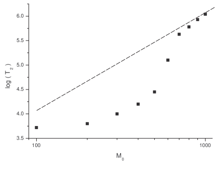
Figure 3: Post-shock temperature at the simulation epoch for different initial Mach numbers. The adiabatic case, $T_{2}\propto M_{0}^{2}$, is shown by dash-line.

In the general case, the high temperature of the post-shock region lead to splash it into the medium. But, in the accretion shock, the infall matter confides the shocked gas so that it may cool and end up with an accretion rotating disk. For finding the relaxation time, we use the equation (3) with $v_{ab}\approx 0$, thus, we have

$$\frac{1}{\gamma_{a}-1}\mathcal{K}_{a}\frac{dT_{a}}{dt}=-\frac{\Lambda_{0}}{(\mu_{a}m_{H})^{2}}\rho_{a}\left(\frac{T_{a}}{T_{0}}\right)^{\beta}.$$ (16)

The temperature of the accreted shocked gas can be obtained by integrating the equation (16). The result is in a piecewise change from $T_{a1}$ (at $t_{1}$) to $T_{a2}$ (at $t_{2}$) as follows:

$$T_{a2}=\{T_{a1}^{1-\beta}-\frac{(1-\beta)(\gamma_{a}-1)}{\mathcal{K}_{a}}\frac{\Lambda_{0}}{(\mu_{a}m_{H})^{2}}\times$$

$$\frac{\rho_{a}}{T_{0}^{\beta}}(t_{2}-t_{1})\}^{\frac{1}{1-\beta}},$$ (17)

which is shown in Fig. 4, with assumption of $\rho_{a}\approx 4$.

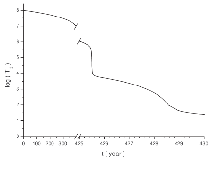
Figure 4: Relaxation of the temperature of the post-shock gas in the head-on collision of two sheets.

4 Summary and conclusions

Molecular cloud cores are rotating so that in the process of collapse and protostellar formation, the infalling matters, which arrive at the equator, collide and dissipate the kinetic energy of motion perpendicular to the equatorial plane so that an accretion disk can be formed. The speed of infalling matters at the equator is so high that the strong supersonic shocks appear, and the temperature of post-shock gas is increased so causing to dissociate the molecules and ionize the atoms. In adiabatic strong supersonic shocks, the density of post-shock region is about fourfold of initial density, and the temperature is increased proportional to the square of the Mach number. On the other hand, the cooling processes of the post-shock gas can decrease the temperature so that the ionized gases can be recombined to form the atoms and molecules, if the duration time-scale of the post-shock region is longer than the cooling time-scale. The suitable cooling function for the post-shock gas (Table 1) showed that the cooling time-scale has a minimum which is at the ranges of ionizing temperature (Fig. 1). This minimum, which is nominated as a trap, causes to cool the post-shock gas in a fast rate. Thus, if the initial speed of colliding matters is so high that the temperature of post-shock gas settles in this trap region, it will quickly cool and electrons recombine with nucleons.

For investigating the time evolution of the post-shock gas in the strong supersonic collisions, which occurs at protostellar accretion shocks, we used the SPH method with the variable artificial viscosity to obtain the more smoothed results of simulations (Fig. 2). The simulations of strong shocks with great Mach numbers show that the temperature of the post-shock gas is quickly increased near to $T_{2}^{max}$, which is for the adiabatic case, and gradually decreased by the time according to the cooling rate. Decrease of temperature of the post-shock gas at the simulation epoch is shown in Fig.3 for different values of the Mach numbers. We see from this figure that the decreasing rate of temperature is very fast in the trap region as depicted by Fig. 1.

The simulations show that the temperature of center of the post-shock gradually decreases, while in the ridges, it stays about $T_{2}^{max}$ because of continuously infall of matters. Temperature decrease of the central region leads to increase of its density in an isobaric manner so that an accretion thin disk can be formed. Thus, over the time, center of the collisional infalling matters (i.e., equatorial plane) converts to a dense molecular thin disk with an atomic envelope and ionized gas which comes from strong shocks of continuous infalling matters. The time in which this structure occurs, depends on the Mach number that is shown in Fig. 4. The temperature range of the trap, which leads to fast cooling of the post-shock gas, is clearly seen in Fig. 4, too. Thus, we see that the cooling processes of the post-shock gas in the protostellar accretion shocks can lead to the formation of an accretion thin molecular disk at the equatorial plane, in a convenient time-scale. This dense molecular thin disk is appropriate for grain coagulation and formation of proto-planetary entities.

References

- [] Akeson, R.L.: 2008, JPhCS 131, 2019
- [] Bate, M.R.: 2010, MNRAS 404, 79
- [] Bondi, H.: 1952, MNRAS 112, 195
- [] Ciardi, A., Hennebelle, P.: 2010, MNRAS 409, 39
- [] Ceccarelli, C., Hollenbach, D.J., Tielens, A.G.G.M.: 1996, ApJ 471, 400
- [] Dalgarno, A., McCray, R.A.: 1972, ARA&A 10, 375
- [] Dunham, M.M., Evans, N.J., Bourke, T.L., Myers, P.C., Huard, T.L., Stutz, A.M.: 2010, ApJ 721, 995
- [] Dyson, J.E., Williams, D.A.: 1997, Physics of the Interstellar Medium, 2nd Edition, IOP publishing Ltd., p. 99
- [] Fatuzzo, M., Adams, F.C., Myers, P.C.: 2004, ApJ 615, 813
- [] Foster, P.N., Chevalier, R.A.: 1993, ApJ 416, 303
- [] Furuya, R.S., Cesaroni, R., Shinnaga, H.: 2011, A&A 525, 72
- [] Galli, D., Shu, F.H.: 1993, ApJ 417, 243
- [] Garrod, R.T., Herbst, E.: 2006, A&A 457, 927
- [] Garrod, R.T., Weaver, S.L.W., Herbst, E.: 2008, ApJ 682, 283
- [] Hartmann, L.: 2009, Accresion Processes in Astrophysics, 2ed, Cambridge University Press
- [] Heitsch, F., Hartmann, L.W., Burkert, A.: 2008, ApJ 683, 786
- [] Henriksen, R., André, P., Bontemps, S.: 1997, A&A 323, 549
- [] Hirth, G.A., Mundt, R., Solf, J.: 1997, A&AS 126, 437
- [] Hollenbach, D., McKee, C.F.: 1979, ApJS 41, 555
- [] Hollenbach, D., Salpeter, E.E.: 1971, ApJ 163, 155
- [] Hujeirat, A.: 1998, A&A 334, 742
- [] Hujeirat, A., Livio, M., Camenzind, M., Burkert, A.: 2003, A&A 408, 415
- [] Lequeux, J.: 2005, The Interstellar Medium, Springer-Verlag Berlin Heidelberg, p. 217
- [] Machida, M.N., Inutsuka, S., Matsumoto, T.: 2007, ApJ 670, 1198
- [] Machida, M.N., Inutsuka, S., Matsumoto, T.: 2010, ApJ 724, 1006
- [] McKee, C.F., Hollenbach, D.J.: 1980, ARA&A 18, 219
- [] Mendoza, S., Tejeda, E., Nagel, E.: 2009, MNRAS 393, 579
- [] Monaghan, J.J.: 1989, J. Comp. Phys. 82, 1
- [] Monaghan, J.J.: 1992, ARA&A 30, 543
- [] Monaghan, J.J.: 2005, Rep. Prog. Phys. 68, 1703
- [] Nejad-Asghar, M.: 2011, MNRAS in press (arXiv1101.5674)
- [] Nejad-Asghar, M.: 2010, RAA 10, 1275
- [] Nejad-Asghar, M., Khesali, A.R., Soltani, J.: 2008, Ap&SS 313, 425
- [] Neufeld, D.A., Hollenbach, D.J.: 1994, ApJ 428, 170
- [] Osterbrock, D.E., Ferland, G.J.: 2006, Astrophysics of Gaseous Nebulae and Active Galactic Nuclei, 2nd Edition, Sausalito, California: University Science Books, p. 22
- [] Quanz, S.P., Beuther, H., Steinacker, J., Linz, H., Birkmann, S.M., Krause, O., Henning, T., Zhang, Q.: 2010, ApJ 717, 693
- [] Rodgers, S.D., Charnley, S.B.: 2003, ApJ 585, 355
- [] Rosswog, S.: 2009, NewA 53, 78
- [] Shu, F.H.: 1977, ApJ 214, 488
- [] Sutherland, R.S., Dopita, M.A.: 1993, ApJS 88, 253
- [] Terebey, S., Shu, F.H., Cassen, P.: 1984, ApJ 286, 529
- [] Ulrich, R.K.: 1976, ApJ 210, 377
- [] Visser, R., van Dishoeck, E.F., Doty, S.D., Dullemond, C.P.: 2009, A&A 495, 881
- [] Walch, S., Burkert, A., Whitworth, A., Naab, T., Gritschneder, M.: 2009, MNRAS 400, 13
- [] Watson, A.M., Stapelfeldt, K.R., Wood, K., Ménard, F.: 2007, prpl.conf, 523
- [] Wolfire, M.G., Hollenbach, D., McKee, C.F., Tielens, A.G.G.M., Bakes, E.L.O.: 1995, ApJ 443, 152
- [] Wu, Y., Wei, Y., Zhao, M., Shi, Y., Yu, W., Qin, S., Huang, M.: 2004, A&A 426, 503