Abstract

Various solutions to the discrete Schwarzian KdV equation are discussed. We first derive the bilinear difference equations of Hirota type of the discrete Schwarzian KP equation, which is decomposed into three discrete two-dimensional Toda lattice equations. We then construct two kinds of solutions in terms of the Casorati determinant. We derive the discrete Schwarzian KdV equation on an inhomogeneous lattice and its solutions by a reduction process. We finally discuss the solutions in terms of the $\tau$ functions of some Painlevé systems.

Keywords and Phrases: discrete Schwarzian KdV equation, discrete Schwarzian KP equation, $\tau$ function, bilinear equation, discrete integrable systems, Painlevé systems.

1 Introduction

The focus of this article is on the partial difference equation

$$\frac{(z_{l_{1},l_{2}}-z_{l_{1}+1,l_{2}})(z_{l_{1}+1,l_{2}+1}-z_{l_{1},l_{2}+1})}{(z_{l_{1}+1,l_{2}}-z_{l_{1}+1,l_{2}+1})(z_{l_{1},l_{2}+1}-z_{l_{1},l_{2}})}=\frac{\lambda(l_{1})}{\mu(l_{2})},$$ (1.1)

known as the discrete Schwarzian KdV equation (dSKdV), where $l_{k}$ ($k=1,2$) are independent variables, $z_{l_{1},l_{2}}$ denotes the value of the dependent variable $z$ at the lattice site $(l_{1},l_{2})$ and $\lambda(l_{1})$ and $\mu(l_{2})$ are arbitrary functions in the indicated variables. As a lattice equation, dSKdV (1.1) was first studied in [21, 19], and classified as a special case of ‘Q1’ equation in the ABS list [1]. It yields the Schwarzian KdV equation

$$\psi_{t}=\psi_{x}S(\psi),\quad S(\psi)\equiv\frac{\psi_{xxx}}{\psi_{x}}-\frac{3}{2}\frac{\psi_{xx}^{2}}{\psi_{x}^{2}},$$ (1.2)

in the continuous limit, and is related to the lattice modified KdV equation and the lattice KdV equation by Miura transformations [22]. Note that the differential operator $S$ in (1.2) is the Schwarzian derivative and thus (1.2) is invariant with respect to Möbius transformations. The soliton equations with Möbius invariance may consequently be called ‘Schwarzian’. See [17] for a review of Schwarzian equations. We sometimes refer to (1.1) as non-autonomous for non-constant $\lambda(l_{1})$ and $\mu(l_{2})$. When $\lambda(l_{1})$ and $\mu(l_{2})$ are both constants, we call it autonomous. dSKdV is also known as the cross-ratio equation, since the left hand side of (1.1) is the cross ratio, which is fundamental to many branches of geometry and was studied as early as the time of Euclid. Our main motive for exploring this system comes from a geometrical setting: dSKdV arises as one of the most basic equations in the discrete differential geometry, which is expected to provide a new mathematical framework of discretization of various geometrical objects. For example, dSKdV is used to define the discrete conformality of discrete isothermic nets [2, 3].

For notational simplicity, we display only the shifted independent variables. For example, $z_{l_{1}+1,l_{2}}$ may be written as $z_{l_{1}+1}$. Using this convention, (1.1) may be written as

$$\frac{(z-z_{l_{1}+1})(z_{l_{1}+1,l_{2}+1}-z_{l_{2}+1})}{(z_{l_{1}+1}-z_{l_{1}+1,l_{2}+1})(z_{l_{2}+1}-z)}=\frac{\lambda(l_{1})}{\mu(l_{2})}.$$ (1.3)

Note that if there exists a function $u_{l_{1},l_{2}}$ satisfying

$$z_{l_{i}+1}-z=f_{i}(l_{i})~{}u_{l_{i}+1}u\quad(i=1,2)$$ (1.4)

where $f_{i}(l_{i})$ ($i=1,2$) are arbitrary functions, then (1.1) is automatically satisfied with $\lambda(l_{1})=f_{1}(l_{1})^{2}$ and $\mu(l_{2})=f_{2}(l_{2})^{2}$.

In this article, we aim to clarify the structure of the bilinear difference equations and $\tau$ functions associated with dSKdV (1.1). We then construct various solutions to dSKdV, including the soliton type solutions of autonomous dSKdV presented in [5, 18]. In section 2, we consider the discrete Schwarzian KP equation (dSKP). We first discuss the bilinear equations and $\tau$ function of dSKP in section 2.1. We then establish the reduction procedure to derive dSKdV from dSKP. In [14] a basic geometric property of circles was shown to be equivalent to dSKP, and dSKdV as a special case. In that article a reduction from dSKP to a degenerate dSKdV was discussed. The full, non-autonomous dSKdV is difficult to achieve via reduction because of complications arising from the non-autonomous terms. However, a method to circumvent these complications was described in [11, 12], where the reduction is performed along auxiliary variables, enabling the reduced equation to remain non-autonomous in its independent variables. We use a similar technique to obtain dSKdV from dSKP by reduction. We thereby construct solutions to (1.1) in the form of $\tau$ functions of the Casorati ($N$-soliton) and molecule types. This is explained in section 2.2.

dSKdV appears not only as one of the discrete soliton equations, but also as the equation describing the chain of Bäcklund transformations of the Painlevé systems. This was first reported in [22] for the case of the Painlevé VI equation, which implies that dSKdV also admits solutions expressible in terms of the $\tau$ functions of the Painlevé VI equation. The same situation also arises for other Painlevé systems. In section 3, we discuss dSKdV in the setting of the Painlevé systems and construct explicit formulae of solutions in terms of their $\tau$ functions. We consider the Painlevé systems with the affine Weyl group symmetry of type $(A_{2}+A_{1})^{(1)}$ and $D_{4}^{(1)}$, where the former includes a $q$-Painlevé III equation, and the latter the Painlevé VI equation.

2 Discrete Schwarzian KP Equation and Its Reduction

2.1 Discrete Schwarzian KP Equation

The discrete Schwarzian KP equation (dSKP) is

$$\frac{(z_{l_{1}+1}-z_{l_{1}+1,l_{2}+1})(z_{l_{2}+1}-z_{l_{2}+1,l_{3}+1})(z_{l_{3}+1}-z_{l_{1}+1,l_{3}+1})}{(z_{l_{1}+1,l_{2}+1}-z_{l_{2}+1})(z_{l_{2}+1,l_{3}+1}-z_{l_{3}+1})(z_{l_{1}+1,l_{3}+1}-z_{l_{1}+1})}=-1$$ (2.1)

where $l_{i}$ $(i=1,2,3)$ are the discrete independent variables and $z=z_{l_{1},l_{2},l_{3}}$ is the dependent variable. dSKP was first published in an alternative form in [20], first appeared in the quoted form in [4] and was also studied by [14]. In the context of discrete differential geometry, $z$ arises as a complex valued function. We first give an explicit formula for the solution of dSKP in terms of a $\tau$ function:

Proposition 2.1.

Let $\tau_{l_{1},l_{2},l_{3}}^{m,s}$ be the $\tau$ function satisfying the following bilinear difference equations:

$$\tau_{l_{i}+1}^{m+1}\tau-\tau_{l_{i}+1}\tau^{m+1}=\tau_{l_{i}+1}^{s+1}\tau^{m+1,s-1}\quad(i=1,2,3),$$ (2.2)

where $m$ and $s$ are the auxiliary independent variables. Then,

$$z_{l_{1},l_{2},l_{3}}=\frac{\tau_{l_{1},l_{2},l_{3}}^{m+1,s}}{\tau_{l_{1},l_{2},l_{3}}^{m,s}},$$ (2.3)

satisfies dSKP (2.1).

Proof.

First note that if there exist some functions $v=v_{l_{1},l_{2},l_{3}}$ and $w=w_{l_{1},l_{2},l_{3}}$ such that

$$z_{l_{i}+1}-z=v_{l_{i}+1}w\quad(i=1,2,3),$$ (2.4)

then (2.1) is automatically satisfied. Dividing (2.2) by $\tau_{l_{i}+1}\tau$ we have

$$\frac{\tau_{l_{i}+1}^{m+1}}{\tau_{l_{i}+1}}-\frac{\tau^{m+1}}{\tau}=\frac{\tau_{l_{i}+1}^{s+1}}{\tau_{l_{i}+1}}\frac{\tau^{m+1,s-1}}{\tau}\quad(i=1,2,3),$$

which is equivalent to (2.4) if we define $v$ and $w$ by

$$v=\frac{\tau^{s+1}}{\tau},\quad w=\frac{\tau^{m+1,s-1}}{\tau},$$ (2.5)

respectively. ∎

Remark 2.2.

dSKP (2.1) is invariant under the change of the independent variables $l_{i}\to-l_{i}$ ($i=1,2,3$). Therefore if the $\tau$ function is a solution to the bilinear equation

$$\tau^{m+1}\tau_{l_{i}+1}-\tau\tau_{l_{i}+1}^{m+1}=\tau^{s+1}\tau_{l_{i}+1}^{m+1,s-1}\quad(i=1,2,3),$$ (2.6)

then $z$ in (2.3) also satisfies (2.1). In this case, $v$ and $w$ in (2.4) are expressed as

$$v=\frac{\tau^{m+1,s-1}}{\tau},\quad w=-\frac{\tau^{s+1}}{\tau}.$$ (2.7)

Each of the bilinear equations in (2.2) is the discrete two-dimensional Toda lattice equation[6] with respect to the independent variables $(l_{i},m,s)$ ($i=1,2,3$). It is therefore possible to construct the Casorati determinant solution to these equations (2.2) as follows [6, 24, 7, 16]:

Theorem 2.3.

Let $\sigma=\sigma_{l_{1},l_{2},l_{3}}^{m,s}$ be an $N\times N$ Casorati determinant defined by

$$\sigma=\left|\begin{array}[]{cccc}\varphi_{1}&\varphi_{1}^{s+1}&\cdots&\varphi_{1}^{s+N-1}\\ \varphi_{2}&\varphi_{2}^{s+1}&\cdots&\varphi_{2}^{s+N-1}\\ \vdots&\vdots&\cdots&\vdots\\ \varphi_{N}&\varphi_{N}^{s+1}&\cdots&\varphi_{N}^{s+N-1}\end{array}\right|,$$ (2.8)

where $\varphi_{i}=\varphi_{i,l_{1},l_{2},l_{3}}^{m,s}$ ($i=1,\ldots,N$) are arbitrary functions satisfying the following linear relations:

$$\frac{\varphi_{i}-\varphi_{i,l_{k}-1}}{a_{k}(l_{k}-1)}=\varphi_{i}^{s+1}\quad(k=1,2,3),$$ (2.9)

$$\frac{\varphi_{i}-\varphi_{i}^{m-1}}{b}=-\varphi_{i}^{s-1}.$$ (2.10)

Here, $a_{k}(l_{k})$ ($k=1,2,3$) are arbitrary functions in the indicated independent variables and $b$ is a constant. Then

$$\tau=\left[\prod_{k=1}^{3}\prod_{j_{k}}^{l_{k}-1}(1+a_{k}(j_{k})b)^{m}a_{k}(j_{k})^{s}\right]b^{-ms}~{}\sigma$$ (2.11)

satisfies the bilinear equations (2.2).

Proof.

It is known that $\sigma$ satisfies the bilinear equation

$$(1+a_{k}(l_{k})b)\sigma_{l_{k}+1}^{m+1}\sigma-\sigma_{l_{k}+1}\sigma^{m+1}=a_{k}(l_{k})b~{}\sigma_{l_{k}+1}^{s+1}\sigma^{m+1,s-1}\quad(k=1,2,3),$$ (2.12)

which follows from an appropriate Plücker relation [7, 16, 23, 24]. From (2.11) it is easily verified that $\tau$ satisfies (2.2). ∎

It is also possible to choose the size of the Casorati determinant as one of the discrete independent variables in $l_{k}$ ($k=1,2,3$). This type of solution is sometimes referred to as the molecule type.

Theorem 2.4.

Let $\kappa=\kappa_{l_{1},l_{2},l_{3}}^{m,s}$ be an $l_{1}\times l_{1}$ Casorati determinant defined by

$$\kappa=\left|\begin{array}[]{cccc}\phi_{1}&\phi_{1}^{s+1}&\cdots&\phi_{1}^{s+l_{1}-1}\\ \phi_{2}&\phi_{2}^{s+1}&\cdots&\phi_{2}^{s+l_{1}-1}\\ \vdots&\vdots&\cdots&\vdots\\ \phi_{l_{1}}&\phi_{l_{1}}^{s+1}&\cdots&\phi_{l_{1}}^{s+l_{1}-1}\end{array}\right|,$$ (2.13)

where $\phi_{i}=\phi_{i,l_{2},l_{3}}^{m,s}$ ($i=1,\ldots,l_{1}$) satisfy the following linear relations:

$$\frac{\phi_{i,l_{k}+1}-\phi_{i}}{c_{k}(l_{k})}=-\phi_{i}^{s+1}\quad(k=2,3),$$ (2.14)

$$\frac{\phi_{i}-\phi_{i}^{m-1}}{b}=-\phi_{i}^{s-1}.$$ (2.15)

Here, $c_{k}(l_{k})$ ($k=2,3$) are arbitrary functions in the indicated independent variables and $b$ is a constant. Then

$$\tau=\left[\prod_{k=2}^{3}\prod_{j_{k}}^{l_{k}-1}(1+c_{k}(j_{k})b)^{-m}c_{k}(j_{k})^{-s}\right]b^{-ms}~{}\kappa$$ (2.16)

satisfies the bilinear equations (2.6).

Proof.

From an appropriate Plücker relation, we can derive the bilinear equation with respect to the independent variables $(l_{1},m,s)$ as

$$\kappa^{m+1}\kappa_{l_{1}+1}-\kappa\kappa_{l_{1}+1}^{m+1}=b~{}\kappa^{s+1}\kappa_{l_{1}+1}^{m+1,s-1}.$$ (2.17)

Since the linear relation (2.14) is essentially obtained by the change of variables $l_{k}\to-l_{k}$ ($k=2,3$) from (2.9), we have

$$(1+c_{k}(l_{k})b)\kappa^{m+1}\kappa_{l_{k}+1}-\kappa\kappa_{l_{k}+1}^{m+1}=c_{k}(l_{k})b~{}\kappa^{s+1}\kappa_{l_{k}+1}^{m+1,s-1}\quad(k=2,3).$$ (2.18)

Therefore $\tau$ defined by (2.16) satisfies (2.6). ∎

2.2 Reduction to Discrete Schwarzian KdV Equation

It is possible to obtain dSKdV by a certain reduction procedure from dSKP (2.1). On the level of $z$, the reduction is achieved by applying three extra conditions, which are obtained by imposing a certain symmetry in each of the independent variables $l_{i}$ ($i=1,2,3$). The symmetry required is such that one of the independent variables $l_{i}$ ($i=1,2,3$) of dSKP (2.1) can be negated in each of three conditions. In fact, only two conditions are needed as the third is redundant, we only mention that there are three such conditions for completeness.

Proposition 2.5.

Let $z_{l_{1},l_{2},l_{3}}$ be a function satisfying (2.1). We impose the following equations for $z$:

$$\frac{(z_{l_{1}+1,l_{2},l_{3}}-z_{l_{1}+1,l_{2}+1,l_{3}})(z_{l_{1},l_{2}+1,l_{3}}-z_{l_{1},l_{2}+1,l_{3}-1})(z_{l_{1},l_{2},l_{3}-1}-z_{l_{1}+1,l_{2},l_{3}-1})}{(z_{l_{1}+1,l_{2}+1,l_{3}}-z_{l_{1},l_{2}+1,l_{3}})(z_{l_{1},l_{2}+1,l_{3}-1}-z_{l_{1},l_{2},l_{3}-1})(z_{l_{1}+1,l_{2},l_{3}-1}-z_{l_{1}+1,l_{2},l_{3}})}=-1,$$ (2.19)

$$\frac{(z_{l_{1}+1,l_{2},l_{3}}-z_{l_{1}+1,l_{2}-1,l_{3}})(z_{l_{1},l_{2}-1,l_{3}}-z_{l_{1},l_{2}-1,l_{3}+1})(z_{l_{1},l_{2},l_{3}+1}-z_{l_{1}+1,l_{2},l_{3}+1})}{(z_{l_{1}+1,l_{2}-1,l_{3}}-z_{l_{1},l_{2}-1,l_{3}})(z_{l_{1},l_{2}-1,l_{3}+1}-z_{l_{1},l_{2},l_{3}+1})(z_{l_{1}+1,l_{2},l_{3}+1}-z_{l_{1}+1,l_{2},l_{3}})}=-1.$$ (2.20)

Then (2.1) is reduced to dSKdV (1.3).

Note that a third condition, with $l_{1}\mapsto-l_{1}$, is consistent with (2.19) and (2.20).

Proof.

Let us fix $l_{3}$ and put $z_{l_{1},l_{2}}=z_{l_{1},l_{2},l_{3}}$, $y_{l_{1},l_{2}}=z_{l_{1},l_{2},l_{3}+1}$. We drop the $l_{3}$ dependence in the expression of $y$ and $z$. Then (2.1), (2.19)${}_{l_{3}+1}$ and (2.20)${}_{l_{2}+1}$ can be written as

$$\frac{(z_{l_{1}+1}-z_{l_{1}+1,l_{2}+1})(z_{l_{2}+1}-y_{l_{2}+1})(y-y_{l_{1}+1})}{(z_{l_{1}+1,l_{2}+1}-z_{l_{2}+1})(y_{l_{2}+1}-y)(y_{l_{1}+1}-z_{l_{1}+1})}=-1,$$ (2.21)

$$\frac{(y_{l_{1}+1}-y_{l_{1}+1,l_{2}+1})(y_{l_{2}+1}-z_{l_{2}+1})(z-z_{l_{1}+1})}{(y_{l_{1}+1,l_{2}+1}-y_{l_{2}+1})(z_{l_{2}+1}-z)(z_{l_{1}+1}-y_{l_{1}+1})}=-1,$$ (2.22)

$$\frac{(z_{l_{1}+1,l_{2}+1}-z_{l_{1}+1})(z-y)(y_{l_{2}+1}-y_{l_{1}+1,l_{2}+1})}{(z_{l_{1}+1}-z)(y-y_{l_{2}+1})(y_{l_{1}+1,l_{2}+1}-z_{l_{1}+1,l_{2}+1})}=-1,$$ (2.23)

respectively. One can eliminate $y$ from (2.21) and (2.22) as follows: we first eliminate $y_{l_{1}+2,l_{2}+1}$ and $y_{l_{1}+1,l_{2}+2}$ from (2.21)${}_{l_{1}+1,l_{2}+1}$ by using (2.22)${}_{l_{1}+1}$ and (2.22)${}_{l_{2}+1}$. In the resulting equation, we use (2.21)${}_{l_{1}+1}$ and (2.21)${}_{l_{2}+1}$ to eliminate $y_{l_{1}+2}$ and $y_{l_{2}+2}$. The resulting expression still contains $y_{l_{1}+1}$, $y_{l_{2}+1}$ and $y_{l_{1}+1,l_{2}+1}$, but they are eliminated by virtue of (2.22), leaving the following expression in $z$ alone

$$\frac{(z_{l_{1}+2,l_{2}+2}-z_{l_{1}+2,l_{2}+1})(z_{l_{1}+1,l_{2}+2}-z_{l_{2}+2})(z_{l_{1}+2}-z_{l_{1}+1})(z_{l_{2}+1}-z)}{(z_{l_{1}+2,l_{2}+2}-z_{l_{1}+1,l_{2}+2})(z_{l_{1}+2,l_{2}+1}-z_{l_{1}+2})(z_{l_{2}+2}-z_{l_{2}+1})(z_{l_{1}+1}-z)}=1.$$ (2.24)

Equation (2.24) is rearranged in the following form

$$\frac{X_{l_{1}+1,l_{2}+1}}{X_{l_{2}+1}}=\frac{X_{l_{1}+1}}{X},$$ (2.25)

$$X=\frac{(z-z_{l_{1}+1})(z_{l_{1}+1,l_{2}+1}-z_{l_{2}+1})}{(z_{l_{1}+1}-z_{l_{1}+1,l_{2}+1})(z_{l_{2}+1}-z)},$$ (2.26)

from which we obtain (1.3). ∎

Note that the ansatz (2.4) is reduced to (1.4) (or (2.36) below) as follows. Substituting (2.4) into the reduction condition (2.19), we have

$$\frac{v_{l_{2}+1}}{w_{l_{2}+1}}~{}\frac{v_{l_{1}+1,l_{3}-1}}{w_{l_{1}+1,l_{3}-1}}=\frac{v_{l_{1}+1}}{w_{l_{1}+1}}~{}\frac{v_{l_{2}+1,l_{3}-1}}{w_{l_{2}+1,l_{3}-1}},$$ (2.27)

which is solved by $w=R(l_{1},l_{2})\rho_{3}(l_{3})v$, causing the ansatz (2.4) to become

$$z_{l_{i}+1}-z=R(l_{1},l_{2})\rho_{3}(l_{3})v_{l_{i}+1}v,$$ (2.28)

where $R(l_{1},l_{2})$ and $\rho_{3}(l_{3})$ are arbitrary functions. Now we apply the additional condition on $z$, (2.23), into which we substitute (2.28). This produces a condition on $R(l_{1},l_{2})$

$$\frac{R_{l_{1}+1,l_{2}+1}R}{R_{l_{1}+1}R_{l_{2}+1}}=1,$$

which implies that $R$ must be separable as $R(l_{1},l_{2})=\rho_{1}(l_{1})\rho_{2}(l_{2})$, where $\rho_{1}(l_{1})$ and $\rho_{2}(l_{2})$ are arbitrary. Now introducing $u=(\rho_{1}(l_{1})\rho_{2}(l_{2})\rho_{3}(l_{3}))^{\frac{1}{2}}v$, (2.28) can be rewritten as

$$z_{l_{i}+1}-z=\left(\frac{\rho_{i}(l_{i})}{\rho_{i}(l_{i}+1)}\right)^{\frac{1}{2}}u_{l_{i}+1}u,$$ (2.29)

which is equivalent to (1.4).

Let us consider the reduction on the level of the $\tau$ function and construct explicit solutions to dSKdV. The above discussion and (2.5) suggests that the reduction condition to be imposed should be $\tau^{m+1}\Bumpeq\tau^{s+2}$, where $\Bumpeq$ means the equivalence up to gauge transformation. However, due to the difference of gauge invariance of the dSKP and dSKdV (and their bilinear equations), the reduction cannot be applied in a straightforward manner. We apply the reduction to the solutions in Theorem 2.3 and 2.4 separately.

We first consider the Casorati determinant solution presented in Theorem 2.3. Choose the entries of the determinant $\sigma$ as

$$\varphi_{i}=\alpha_{i}p_{i}^{s}\prod_{k=1}^{3}\prod_{j_{k}}^{l_{k}-1}(1-a_{k}(j_{k})p_{i})^{-1}\left(1+\frac{b}{p_{i}}\right)^{-m}+\beta_{i}q_{i}^{s}\prod_{k=1}^{3}\prod_{j_{k}}^{l_{k}-1}(1-a_{k}(j_{k})q_{i})^{-1}\left(1+\frac{b}{q_{i}}\right)^{-m},$$ (2.30)

where $p_{i},q_{i},\alpha_{i},\beta_{i}$ ($i=1,\ldots,N$) are constants. We next impose the condition

$$\varphi_{i}^{m+1}\Bumpeq\varphi_{i}^{s+2},$$ (2.31)

which can be realized by choosing the parameters as

$$q_{i}=-p_{i}-b.$$ (2.32)

Equation (2.31) implies the following condition on $\sigma$:

$$\sigma^{m+1}=C_{N}~{}\sigma^{s+2},\quad C_{N}=\prod_{i=1}^{N}p_{i}^{-2}\left(1+\frac{b}{p_{i}}\right)^{-1}.$$ (2.33)

Using (2.33) to eliminate the $m$-dependence and neglecting $l_{3}$-dependence, equations (2.12) are reduced to

$$(1+a_{k}(l_{k})b)\sigma_{l_{k}+1}^{s+2}\sigma-\sigma_{l_{k}+1}\sigma^{s+2}=a_{k}(l_{k})b~{}\sigma_{l_{k}+1}^{s+1}\sigma^{s+1}\quad(k=1,2).$$ (2.34)

Introducing $z=z_{l_{1},l_{2}}$ by

$$z=\prod_{k=1}^{2}\prod_{j_{k}}^{l_{k}-1}(1+a_{k}(j_{k})b)~{}\frac{\sigma^{s+2}}{\sigma},$$ (2.35)

then (2.34) can be rewritten as

$$z_{l_{k}+1}-z=\frac{a_{k}(l_{k})b}{(1+a_{k}(l_{k})b)^{\frac{1}{2}}}~{}u_{l_{k}+1}u\quad(k=1,2),$$ (2.36)

where

$$u=\prod_{k=1}^{2}\prod_{j_{k}}^{l_{k}-1}(1+a_{k}(j_{k})b)^{\frac{1}{2}}~{}\frac{\sigma^{s+1}}{\sigma}.$$ (2.37)

From (2.36), we see that $z$ satisfies dSKdV (1.3) with $\lambda(l_{1})=a_{1}(l_{1})^{2}/(1+a_{1}(l_{1})b)$ and $\mu(l_{2})=a_{2}(l_{2})^{2}/(1+a_{2}(l_{2})b)$. Summarizing the discussion, we have the following theorem:

Theorem 2.6.

Let $\sigma=\sigma_{l_{1},l_{2}}^{s}$ be an $N\times N$ determinant given by

$$\sigma=\det(\varphi_{i,l_{1},l_{2}}^{s+j-1})_{i,j=1,\ldots,N},$$ (2.38)

$$\varphi_{i,l_{1},l_{2}}^{s}=\alpha_{i}p_{i}^{s}\prod_{k=1}^{2}\prod_{j_{k}}^{l_{k}-1}(1-a_{k}(j_{k})p_{i})^{-1}+\beta_{i}q_{i}^{s}\prod_{k=1}^{2}\prod_{j_{k}}^{l_{k}-1}(1-a_{k}(j_{k})q_{i})^{-1},$$ (2.39)

where $p_{i},q_{i},\alpha_{i},\beta_{i}$ are constants, $a_{k}(l_{k})$ ($k=1,2$) are arbitrary functions in the indicated variables and the parameters $p_{i}$ and $q_{i}$ are related as in (2.32). Then $\sigma$ satisfies the bilinear equations (2.34), and $z=z_{l_{1},l_{2}}$ defined by (2.35) satisfies dSKdV (1.3) with $\lambda(l_{1})=a_{1}(l_{1})^{2}/(1+a_{1}(l_{1})b)$ and $\mu(l_{2})=a_{2}(l_{2})^{2}/(1+a_{2}(l_{2})b)$.

We note that the soliton solutions to the autonomous case have been obtained in [5, 18]. Similarly, one can construct the molecule type solution by applying the reduction to the solution in Theorem 2.4.

Theorem 2.7.

Let $\kappa=\kappa_{l_{1},l_{2}}^{s}$ be an $l_{1}\times l_{1}$ determinant given by

$$\kappa=\det(\phi_{i,l_{2}}^{s+j-1})_{i,j=1,\ldots,l_{1}},$$ (2.40)

$$\phi_{i}^{s}= \alpha_{i}p_{i}^{s}\prod_{j}^{l_{2}-1}(1-c_{2}(j)p_{i})+\beta_{i}q_{i}^{s}\prod_{j}^{l_{2}-1}(1-c_{2}(j)q_{i}),$$ (2.41)

where $p_{i},q_{i},\alpha_{i},\beta_{i}$ are constants, $c_{2}(l_{2})$ is an arbitrary function in $l_{2}$ and the parameters $p_{i}$ and $q_{i}$ are related as in (2.32). Then $\kappa$ satisfies the bilinear equations

$$c_{1}(l_{1})\kappa^{s+2}\kappa_{l_{1}+1}-\kappa\kappa_{l_{1}+1}^{s+2}=b~{}\kappa^{s+1}\kappa_{l_{1}+1}^{s+1},$$ (2.42)

$$(1+c_{2}(l_{2})b)\kappa^{s+2}\kappa_{l_{2}+1}-\kappa\kappa_{l_{2}+1}^{s+2}=c_{2}(l_{2})b~{}\kappa^{s+1}\kappa_{l_{2}+1}^{s+1},$$ (2.43)

where

$$c_{1}(l_{1})=p_{l_{1}+1}^{2}\left(1+\frac{b}{p_{l_{1}+1}}\right).$$ (2.44)

Moreover,

$$z_{l_{1},l_{2}}=\prod_{j_{1}}^{l_{1}-1}c_{1}(j_{1})^{-1}\prod_{j_{2}}^{l_{2}-1}(1+a_{2}(j_{2})b)^{-1}~{}\frac{\kappa^{s+2}}{\kappa},$$ (2.45)

satisfies dSKdV (1.3) with $\lambda(l_{1})=c_{1}(l_{1})^{-1}$ and $\mu(l_{2})=c_{2}(l_{2})^{2}/(1+c_{2}(l_{2}))$.

The reduction process to dSKdV is somewhat delicate. For the case of dSKP, the coefficients of the bilinear equations can be removed by multiplying a certain gauge factor to the $\tau$ function. For example, the bilinear equations (2.12) yield (2.2) by using (2.11). For dSKdV, however, such a gauge transformation does not work. For example, the bilinear equations (2.34) can be rewritten as

$$\hat{\tau}_{l_{k}+1}^{s+2}\hat{\tau}-\hat{\tau}_{l_{k}+1}\hat{\tau}^{s+2}=\frac{a_{k}(l_{k})b}{(1+a_{k}(l_{k})b)^{\frac{1}{2}}}~{}\hat{\tau}_{l_{k}+1}^{s+1}\hat{\tau}^{s+1}\ (k=1,2),$$ (2.46)

by introducing $\hat{\tau}=\hat{\tau}_{l_{1},l_{2}}^{s}$ by

$$\hat{\tau}=\prod_{k=1}^{2}\prod_{j_{k}}^{l_{k}-1}(1+a_{k}(j_{k})b)^{\frac{s}{2}}~{}\sigma.$$ (2.47)

Then we have

$$z_{l_{k}+1}-z=\frac{a_{k}(l_{k})b}{(1+a_{k}(l_{k})b)^{\frac{1}{2}}}~{}u_{l_{k}+1}u,$$ (2.48)

where

$$z=\frac{\hat{\tau}^{s+2}}{\hat{\tau}},\quad u=\frac{\hat{\tau}^{s+1}}{\hat{\tau}}.$$ (2.49)

The crucial difference from the case of dSKP is that the coefficient of the right hand side of (2.46) cannot be removed by multiplying a gauge factor to $\tau$. Even for the autonomous case, namely the case where $a_{k}(l_{k})$ are constants, it is possible to remove the coefficient of one of the two bilinear equations, but not possible to remove those of two equations simultaneously.

Therefore, it is not appropriate to impose the condition $\tau^{m+1}\Bumpeq\tau^{s+2}$ on the bilinear equations (2.2). Actually it is obvious that the bilinear equations (2.46) cannot be obtained from naive reduction from (2.2). We have to apply the reduction to the Casorati determinant without its gauge factor instead of applying directly to $\tau_{l_{1},l_{2},l_{3}}^{m,s}$ itself. Such inconsistencies involving gauge factors arising through the reduction process can be seen for other non-autonomous discrete integrable systems as well [11, 12].

Remark 2.8.

Konopelchenko and Schief discussed in [14] the reduction from dSKP to the dSKdV by imposing the condition

$$z_{l_{2}+1,l_{3}+1}=z,$$ (2.50)

on (2.1). Using this condition to eliminate the $l_{3}$ dependence, (2.1) can be rearranged in the form

$$\frac{Y_{l_{2}-1}}{Y}=1,\quad Y=\frac{(z-z_{l_{1}+1})(z_{l_{1}+1,l_{2}+1}-z_{l_{2}+1})}{(z_{l_{1}+1}-z_{l_{1}+1,l_{2}+1})(z_{l_{2}+1}-z)},$$ (2.51)

which yields the special case of (1.3)

$$\frac{(z-z_{l_{1}+1})(z_{l_{1}+1,l_{2}+1}-z_{l_{2}+1})}{(z_{l_{1}+1}-z_{l_{1}+1,l_{2}+1})(z_{l_{2}+1}-z)}=\nu(l_{1}),$$ (2.52)

where $\nu(l_{1})$ is an arbitrary function. The condition (2.50) is the subcase of the condition (2.19): it is easily verified that if $z$ satisfies (2.50) then (2.19) is automatically satisfied. For the solution of dSKP given in Theorem 2.3, it can be shown that (2.50) is realized by taking $a_{k}(l_{k})=a_{k}={\rm const.}$ ($k=2,3$), imposing (2.32), and choosing $b$ as $b=-(\frac{1}{a_{2}}+\frac{1}{a_{3}})$.

3 Discrete Schwarzian KdV Equation in Painlevé Systems

In this section, we consider the solutions of dSKdV which are expressed by $\tau$ functions of certain Painlevé systems. We give two examples, one with the symmetry of the affine Weyl group of type $(A_{2}+A_{1})^{(1)}$, the other with that of type $D_{4}^{(1)}$, and construct explicit formulae of solutions in terms of their $\tau$ functions. We note that these solutions are not directly related to ones discussed in the previous section.

3.1 Painlevé System of Type $(A_{2}+A_{1})^{(1)}$

The Painlevé system of type $(A_{2}+A_{1})^{(1)}$ [8, 9, 10, 13, 25] arises as a family of Bäcklund transformations associated with a $q$-Painlevé III equation

$$\begin{split}&g_{n+1}=\frac{q^{2N+1}c^{2}}{f_{n}g_{n}}\frac{1+a_{0}q^{n}f_{n}}{a_{0}q^{n}+f_{n}},\\ &f_{n+1}=\frac{q^{2N+1}c^{2}}{f_{n}g_{n+1}}\frac{1+a_{0}a_{2}q^{n-m}g_{n+1}}{a_{0}a_{2}q^{n-m}+g_{n+1}},\end{split}$$ (3.1)

for the unknown functions $f_{n}=f_{n}(m,N)$, $g_{n}=g_{n}(m,N)$ and the independent variable $n\in\mathbb{Z}$. Here, $m,N\in\mathbb{Z}$ and $a_{0},a_{2},c,q\in\mathbb{C}^{\times}$ are parameters. The system of equations (3.1) and its Bäcklund transformations can be formulated as a birational representation of the extended affine Weyl group of type $(A_{2}+A_{1})^{(1)}$. We define the transformations $s_{i}$ ($i=0,1,2$) and $\pi$ on variables $f_{j}$ ($j=0,1,2$) and parameters $a_{k}$ ($k=0,1,2$) by

$$\begin{array}[]{ll}{\displaystyle s_{i}(a_{j})=a_{j}a_{i}^{-a_{ij}}},&{\displaystyle s_{i}(f_{j})=f_{j}\left(\frac{a_{i}+f_{j}}{1+a_{i}f_{j}}\right)^{u_{ij}},}\\[5.69054pt] {\displaystyle\pi(a_{j})=a_{j+1}},&{\displaystyle\pi(f_{j})=f_{j+1},}\end{array}$$ (3.2)

for $i,j\in\mathbb{Z}/3\mathbb{Z}$. Here, $A=(a_{ij})_{i,j=0,1,2}$ and $U=(u_{ij})_{i,j=0,1,2}$ are given by

$$A=\left(\begin{array}[]{ccc}2&-1&-1\\ -1&2&-1\\ -1&-1&2\end{array}\right),$$ (3.6)

$$U=\left(\begin{array}[]{ccc}0&1&-1\\ -1&0&1\\ 1&-1&0\end{array}\right),$$ (3.10)

which are the Cartan matrix of type $A_{2}^{(1)}$ and the orientation matrix of the corresponding Dynkin diagram, respectively. We also define the transformations $w_{0}$, $w_{1}$ and $r$ by

$$\begin{split}&w_{0}(f_{i})=\frac{a_{i}a_{i+1}(a_{i-1}a_{i}+a_{i-1}f_{i}+f_{i-1}f_{i})}{f_{i-1}(a_{i}a_{i+1}+a_{i}f_{i+1}+f_{i}f_{i+1})},\\ &w_{1}(f_{i})=\frac{1+a_{i}f_{i}+a_{i}a_{i+1}f_{i}f_{i+1}}{a_{i}a_{i+1}f_{i+1}(1+a_{i-1}f_{i-1}+a_{i-1}a_{i}f_{i-1}f_{i})},\\ &r(f_{i})=\frac{1}{f_{i}},\\ &w_{0}(a_{i})=a_{i},\quad w_{1}(a_{i})=a_{i},\quad r(a_{i})=a_{i},\end{split}$$ (3.11)

for $i\in\mathbb{Z}/3\mathbb{Z}$. Then the group of birational transformations $\langle s_{0},s_{1},s_{2},\pi,w_{0},w_{1},r\rangle$ form the extended affine Weyl group $\widetilde{W}((A_{2}+A_{1})^{(1)})$, namely the transformations satisfy the fundamental relations

$$\begin{split}&s_{i}^{2}=1,\ (s_{i}s_{i+1})^{3}=1,\ \pi^{3}=1,\ \pi s_{i}=s_{i+1}\pi,\\ &w_{0}^{2}=w_{1}^{2}=r^{2}=1,\ rw_{0}=w_{1}r,\end{split}$$ (3.12)

for $i\in\mathbb{Z}/3\mathbb{Z}$, and the actions of $\langle s_{0},s_{1},s_{2},\pi\rangle=\widetilde{W}(A_{2}^{(1)})$ and $\langle w_{0},w_{1},r\rangle=\widetilde{W}(A_{1}^{(1)})$ commute with each other. Note that

$$a_{0}a_{1}a_{2}=q,\quad f_{0}f_{1}f_{2}=qc^{2}$$ (3.13)

are invariant with respect to the action of $\widetilde{W}\left((A_{2}+A_{1})^{(1)}\right)$ and $\widetilde{W}(A_{2}^{(1)})$, respectively. We define the translation operators $T_{i}$ ($i=1,2,3,4$) by

$$T_{1}=\pi s_{2}s_{1},\ T_{2}=s_{1}\pi s_{2},\ T_{3}=s_{1}s_{2}\pi,\ T_{4}=rw_{0},$$ (3.14)

whose actions on parameters $a_{i}$ $(i=0,1,2)$ and $c$ are given by

$$\begin{array}[]{l}T_{1}:~{}(a_{0},a_{1},a_{2},c)\mapsto(qa_{0},q^{-1}a_{1},a_{2},c),\\ T_{2}:~{}(a_{0},a_{1},a_{2},c)\mapsto(a_{0},qa_{1},q^{-1}a_{2},c),\\ T_{3}:~{}(a_{0},a_{1},a_{2},c)\mapsto(q^{-1}a_{0},a_{1},qa_{2},c),\\ T_{4}:~{}(a_{0},a_{1},a_{2},c)\mapsto(a_{0},a_{1},a_{2},qc),\end{array}$$ (3.15)

respectively. Note that $T_{i}$ ($i=1,2,3,4$) commute with each other and $T_{1}T_{2}T_{3}=1$. The action of $T_{1}$ on $f$-variables can be expressed as

$$\begin{split}&T_{1}(f_{1})=\frac{qc^{2}}{f_{1}f_{0}}~{}\frac{1+a_{0}f_{0}}{a_{0}+f_{0}},\\ &T_{1}(f_{0})=\frac{qc^{2}}{f_{0}T_{1}(f_{1})}~{}\frac{1+a_{2}a_{0}T_{1}(f_{1})}{a_{2}a_{0}+T_{1}(f_{1})}.\end{split}$$ (3.16)

Or, applying $T_{1}^{n}T_{2}^{m}T_{4}^{N}$ to (3.16) and putting

$$T_{1}^{n}T_{2}^{m}T_{4}^{N}(f_{i})=f_{i,n,m}^{N}\quad(i=0,1,2),$$ (3.17)

we obtain

$$\begin{split}&f_{1,n+1}=\frac{q^{2N+1}c^{2}}{f_{1}f_{0}}~{}\frac{1+a_{0}q^{n}f_{0}}{a_{0}q^{n}+f_{0}},\\ &f_{0,n+1}=\frac{q^{2N+1}c^{2}}{f_{0}f_{1,n+1}}~{}\frac{1+a_{2}a_{0}q^{n-m}f_{1,n+1}}{a_{2}a_{0}q^{n-m}+f_{1,n+1}},\end{split}$$ (3.18)

which is equivalent to $q$-P_III (3.1). Here, we have employed the convention to display only the shifted variables in $(n,m,N)$.

It is possible to introduce the $\tau$ functions and lift the above representation of the affine Weyl group on the level of the $\tau$ functions. We introduce the new variable $\tau_{i}$ and $\overline{\tau}_{i}$ ($i\in\mathbb{Z}/3\mathbb{Z}$) with

$$f_{i}=q^{\frac{1}{3}}c^{\frac{2}{3}}~{}\frac{\overline{\tau}_{i+1}\tau_{i-1}}{\tau_{i+1}\overline{\tau}_{i-1}}.$$ (3.19)

Then the lift of the representation is realized by the following formulae:

$$\begin{split}&s_{i}(\tau_{i})=u_{i}^{\frac{1}{2}}\left(1+\frac{f_{i}}{a_{i}}\right)\frac{\tau_{i+1}\overline{\tau}_{i-1}}{\overline{\tau}_{i}},\\ &s_{i}(\overline{\tau}_{i})=v_{i}^{-\frac{1}{2}}\left(1+a_{i}f_{i}\right)\frac{\tau_{i+1}\overline{\tau}_{i-1}}{\tau_{i}},\\ &s_{i}(\tau_{j})=\tau_{j},\quad s_{i}(\overline{\tau}_{j})=\overline{\tau}_{j}\ (i\neq j),\end{split}$$ (3.20)

$$\begin{split}&w_{0}(\overline{\tau}_{i})=\left(\frac{a_{i+1}}{a_{i-1}}\right)^{\frac{1}{3}}u_{i-1}\left(1+\frac{f_{i-1}}{a_{i-1}}+\frac{f_{i-1}f_{i+1}}{a_{i-1}a_{i+1}}\right)\frac{\tau_{i}\tau_{i-1}}{\overline{\tau}_{i-1}},\\ &w_{1}(\tau_{i})=\left(\frac{a_{i+1}}{a_{i-1}}\right)^{\frac{1}{3}}v_{i+1}^{-1}\left(1+a_{i-1}f_{i-1}+a_{i-1}a_{i+1}f_{i-1}f_{i+1}\right)\frac{\overline{\tau}_{i}\overline{\tau}_{i+1}}{\tau_{i+1}},\\ &w_{0}(\tau_{i})=\tau_{i},\ w_{1}(\overline{\tau}_{i})=\overline{\tau}_{i},\ r(\tau_{i})=\tau_{i},\ r(\overline{\tau}_{i})=\overline{\tau_{i}},\end{split}$$ (3.21)

where

$$u_{i}=q^{-\frac{1}{3}}c^{-\frac{2}{3}}a_{i},\quad v_{i}=q^{\frac{1}{3}}c^{\frac{2}{3}}a_{i}.$$ (3.22)

We define the $\tau$ function on the lattice of type $A_{2}\times A_{1}$ by

$$T_{1}^{n}T_{2}^{m}T_{4}^{N}(\tau_{1})=\tau_{n,m}^{N}.$$ (3.23)

Note that $\tau_{0}=\tau_{-1,0}^{0}$, $\tau_{1}=\tau_{0,0}^{0}$, $\tau_{2}=\tau_{0,1}^{0}$, $\overline{\tau}_{0}=\tau_{-1,0}^{1}$, $\overline{\tau}_{1}=\tau_{0,0}^{1}$ and $\overline{\tau}_{2}=\tau_{0,1}^{1}$ (Fig.1).

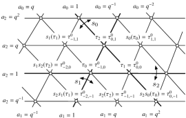
Figure 1: Configuration of the $\tau$ functions on the lattice with $N=0$.

From this construction, it follows that the $\tau$ functions satisfy various bilinear difference equations, we refer to [13] for the list of these.

Now we show that dSKdV arises in the Painlevé system of type $(A_{2}+A_{1})^{(1)}$:

Theorem 3.1.

1. The $\tau$ function satisfies the following bilinear equations:

   $$\tau^{N+1}\tau_{n+1}^{N-1}-Q^{4N}\gamma^{4}\tau_{n+1}^{N+1}\tau^{N-1}+Q^{4n-2m-4N}\gamma^{-4}\alpha_{0}^{6}\alpha_{1}^{2}\alpha_{2}^{4}(Q^{12N}\gamma^{12}-1)\tau_{n+1}\tau=0,$$ (3.24)

   $$\tau^{N+1}\tau_{m+1}^{N-1}-Q^{4N}\gamma^{4}\tau_{m+1}^{N+1}\tau^{N-1}+Q^{4m-2n-4N}\gamma^{-4}\alpha_{1}^{2}\alpha_{2}^{-2}(Q^{12N}\gamma^{12}-1)\tau_{m+1}\tau=0.$$ (3.25)

   Here,

   $$\alpha_{i}=a_{i}^{\frac{1}{6}},\quad\gamma=c^{\frac{1}{6}},\quad Q=q^{\frac{1}{6}}.$$ (3.26)

2. We introduce $z=z_{n,m}$ by

   $$z=(Q^{4N+4}\gamma^{4})^{n+m}~{}\frac{\tau^{N+2}}{\tau}.$$ (3.27)

   Then $z$ satisfies dSKdV

   $$\frac{(z-z_{n+1})(z_{n+1,m+1}-z_{m+1})}{(z_{n+1}-z_{n+1,m+1})(z_{m+1}-z)}=q^{2n-2m}a_{0}^{2}a_{2}^{2}.$$ (3.28)

Proof.

We take (B.17) and (B.20) of [13]:

$$\tau_{n+1}^{N+1}\tau^{N-1}-Q^{m-2n-2N}\gamma^{-2}{\alpha_{0}}^{-3}{\alpha_{1}}^{-1}{\alpha_{2}}^{-2}\tau_{n+1,m+1}\tau_{m-1}-Q^{4n-2m+4N}\gamma^{4}{\alpha_{0}}^{6}{\alpha_{1}}^{2}{\alpha_{2}}^{4}\tau_{n+1}\tau=0,$$ (3.29)

$$\tau^{N+1}\tau_{n+1}^{N-1}-Q^{-2n+m+2N}\gamma^{2}{\alpha_{0}}^{-3}{\alpha_{1}}^{-1}{\alpha_{2}}^{-2}\tau_{m-1}\tau_{n+1,m+1}-Q^{4n-2m-4N}\gamma^{-4}{\alpha_{0}}^{6}{\alpha_{1}}^{2}{\alpha_{2}}^{4}\tau\tau_{n+1}=0.$$ (3.30)

We obtain (3.24) by eliminating $\tau_{n+1,m+1}\tau_{m-1}$ from the above equations. Similarly, (3.25) can be derived by taking (B.18) and (B.21) of [13],

$$\tau_{m+1}^{N+1}\tau^{N-1}-Q^{n-2m-2N}\gamma^{-2}{\alpha_{1}}^{-1}\alpha_{2}\tau_{n-1}\tau_{n+1,m+1}-Q^{-2n+4m+4N}\gamma^{4}{\alpha_{1}}^{2}{\alpha_{2}}^{-2}\tau_{m+1}\tau=0,$$ (3.31)

$$\tau^{N+1}\tau_{m+1}^{N-1}-Q^{n-2m+2N-1}\gamma^{2}\alpha_{0}{\alpha_{2}}^{2}\tau_{n+1,m+1}\tau_{n-1}-Q^{-2n+4m-4N+2}\gamma^{-4}{\alpha_{0}}^{-2}{\alpha_{2}}^{-4}\tau\tau_{m+1}=0,$$ (3.32)

and eliminating $\tau_{n+1,m+1}\tau_{n-1}$. Dividing (3.24) and (3.25) by $\tau_{n+1}^{N-1}\tau^{N-1}$ and $\tau_{m+1}^{N-1}\tau^{N-1}$, respectively, shifting $N\to N+1$, and using (3.27), we have

$$z-z_{n+1}= -(Q^{4N+4}\gamma^{4})^{n+m}Q^{4n-2m-4N-4}\gamma^{-4}\alpha_{0}^{6}\alpha_{1}^{2}\alpha_{2}^{4}(Q^{12N+12}\gamma^{12}-1)u_{n+1}u,$$ (3.33)

$$z-z_{m+1}= -(Q^{4N+4}\gamma^{4})^{n+m}Q^{4m-2n-4N-4}\gamma^{-4}\alpha_{1}^{2}\alpha_{2}^{-2}(Q^{12N+12}\gamma^{12}-1)u_{m+1}u,$$ (3.34)

where

$$u=\frac{\tau^{N+1}}{\tau}.$$ (3.35)

Then it is easy to verify from (3.33) and (3.34) that $z$ actually satisfies (3.28). ∎

3.2 Painlevé System of Type $D_{4}^{(1)}$

The relationship between dSKdV

$$\dfrac{(z_{n,m}-z_{n+1,m})(z_{n+1,m+1}-z_{n,m+1})}{(z_{n+1,m}-z_{n+1,m+1})(z_{n,m+1}-z_{n,m})}=\dfrac{1}{t},$$ (3.36)

and the sixth Painlevé equation (P_VI)

$$\begin{array}[]{l}\dfrac{d^{2}q}{dt^{2}}=\dfrac{1}{2}\left(\dfrac{1}{q}+\dfrac{1}{q-1}+\dfrac{1}{q-t}\right)\!\!\left(\dfrac{dq}{dt}\right)^{2}\\[11.38109pt] ~{}-\left(\dfrac{1}{t}+\dfrac{1}{t-1}+\dfrac{1}{q-t}\right)\!\dfrac{dq}{dt}+\dfrac{q(q-1)(q-t)}{2t^{2}(t-1)^{2}}\\[11.38109pt] ~{}\times\left[\kappa_{\infty}^{2}-\kappa_{0}^{2}\dfrac{t}{q^{2}}+\kappa_{1}^{2}\dfrac{t-1}{(q-1)^{2}}+(1-\theta^{2})\dfrac{t(t-1)}{(q-t)^{2}}\right]\end{array}$$ (3.37)

is discussed in [22]. In a word, dSKdV is a part of the Bäcklund transformations of P_VI, which is formulated as a birational representation of the extended affine Weyl group of type $D_{4}^{(1)}$. In this subsection, we construct a class of the particular solutions to dSKdV in terms of the $\tau$ functions of P_VI.

As a preparation, we give a brief review of the Bäcklund transformations and some of the bilinear equations for the $\tau$ functions [15]. It is well-known that P_VI (3.37) is equivalent to the Hamilton system

$$q^{\prime}=\dfrac{\partial H}{\partial p},\quad p^{\prime}=-\dfrac{\partial H}{\partial q},\quad^{\prime}=t(t-1)\dfrac{d}{dt},$$ (3.38)

whose Hamiltonian is given by

$$H=f_{0}f_{3}f_{4}f_{2}^{2}-[\alpha_{4}f_{0}f_{3}+\alpha_{3}f_{0}f_{4}+(\alpha_{0}-1)f_{3}f_{4}]f_{2}+\alpha_{2}(\alpha_{1}+\alpha_{2})f_{0}.$$ (3.39)

Here $f_{i}$ and $\alpha_{i}$ are defined by

$$f_{0}=q-t,\quad f_{3}=q-1,\quad f_{4}=q,\quad f_{2}=p,$$ (3.40)

and

$$\alpha_{0}=\theta,\quad\alpha_{1}=\kappa_{\infty},\quad\alpha_{3}=\kappa_{1},\quad\alpha_{4}=\kappa_{0}$$ (3.41)

with $\alpha_{0}+\alpha_{1}+2\alpha_{2}+\alpha_{3}+\alpha_{4}=1$. The Bäcklund transformations of P_VI are described by

$$s_{i}(\alpha_{j})=\alpha_{j}-a_{ij}\alpha_{i}\quad(i,j=0,1,2,3,4),$$ (3.42)

$$s_{2}(f_{i})=f_{i}+\dfrac{\alpha_{2}}{f_{2}},\quad s_{i}(f_{2})=f_{2}-\dfrac{\alpha_{i}}{f_{i}}~{}~{}(i=0,3,4),$$ (3.43)

$$\begin{array}[]{ll}s_{5}:\!\!\!\!&\alpha_{0}\leftrightarrow\alpha_{1},\quad\alpha_{3}\leftrightarrow\alpha_{4},\\[5.69054pt] &f_{2}\mapsto-\dfrac{f_{0}(f_{2}f_{0}+\alpha_{2})}{t(t-1)},\quad f_{4}\mapsto t\dfrac{f_{3}}{f_{0}},\\[8.53581pt] s_{6}:\!\!\!\!&\alpha_{0}\leftrightarrow\alpha_{3},\quad\alpha_{1}\leftrightarrow\alpha_{4},\\[5.69054pt] &f_{2}\mapsto-\dfrac{f_{4}(f_{4}f_{2}+\alpha_{2})}{t},\quad f_{4}\mapsto\dfrac{t}{f_{4}},\\[8.53581pt] s_{7}:\!\!\!\!&\alpha_{0}\leftrightarrow\alpha_{4},\quad\alpha_{1}\leftrightarrow\alpha_{3},\\[5.69054pt] &f_{2}\mapsto\dfrac{f_{3}(f_{3}f_{2}+\alpha_{2})}{t-1},\quad f_{4}\mapsto\dfrac{f_{0}}{f_{3}},\end{array}$$ (3.44)

where $A=(a_{ij})_{i,j=0}^{4}$ is the Cartan matrix of type $D^{(1)}_{4}$. Then the group of birational transformations $\langle s_{0},\ldots,s_{7}\rangle$ generate the extended affine Weyl group $\widetilde{W}(D^{(1)}_{4})$. In fact, these generators satisfy the fundamental relations

$$\begin{array}[]{l}s_{i}^{2}=1\quad(i=0,\ldots,7),\\ s_{i}s_{2}s_{i}=s_{2}s_{i}s_{2}\quad(i=0,1,3,4),\end{array}$$ (3.45)

and

$$\begin{array}[]{l}s_{5}s_{\{0,1,2,3,4\}}=s_{\{1,0,2,4,3\}}s_{5},\\ s_{6}s_{\{0,1,2,3,4\}}=s_{\{3,4,2,0,1\}}s_{6},\\ s_{7}s_{\{0,1,2,3,4\}}=s_{\{4,3,2,1,0\}}s_{7},\\[2.84526pt] s_{5}s_{6}=s_{6}s_{5},\quad s_{5}s_{7}=s_{7}s_{5},\quad s_{6}s_{7}=s_{7}s_{6}.\end{array}$$ (3.46)

Let us introduce the variables $\tau_{i}\,(i=0,1,2,3,4)$ via the Hamiltonian, so that the action of $\widetilde{W}(D^{(1)}_{4})$ is given by

$$\begin{array}[]{l}s_{0}(\tau_{0})=f_{0}\dfrac{\tau_{2}}{\tau_{0}},\quad s_{1}(\tau_{1})=\dfrac{\tau_{2}}{\tau_{1}},\\[8.53581pt] s_{2}(\tau_{2})=\dfrac{f_{2}}{\sqrt{t}}\dfrac{\tau_{0}\tau_{1}\tau_{3}\tau_{4}}{\tau_{2}},\\[8.53581pt] s_{3}(\tau_{3})=f_{3}\dfrac{\tau_{2}}{\tau_{3}},\quad s_{4}(\tau_{4})=f_{4}\dfrac{\tau_{2}}{\tau_{4}},\end{array}$$ (3.47)

and

$$\begin{array}[]{ll}s_{5}:\!\!\!\!&\tau_{0}\mapsto[t(t-1)]^{\frac{1}{4}}\tau_{1},\quad\tau_{1}\mapsto[t(t-1)]^{-\frac{1}{4}}\tau_{0},\\[2.84526pt] &\tau_{3}\mapsto t^{-\frac{1}{4}}(t-1)^{\frac{1}{4}}\tau_{4},\quad\tau_{4}\mapsto t^{\frac{1}{4}}(t-1)^{-\frac{1}{4}}\tau_{3},\\[2.84526pt] &\tau_{2}\mapsto[t(t-1)]^{-\frac{1}{2}}f_{0}\tau_{2},\end{array}$$ (3.48)

$$\begin{array}[]{ll}s_{6}:\!\!\!\!&\tau_{0}\mapsto it^{\frac{1}{4}}\tau_{3},\quad\tau_{3}\mapsto-it^{-\frac{1}{4}}\tau_{0},\\[2.84526pt] &\tau_{1}\mapsto t^{-\frac{1}{4}}\tau_{4},\quad\tau_{4}\mapsto t^{\frac{1}{4}}\tau_{1},\quad\tau_{2}\mapsto t^{-\frac{1}{2}}f_{4}\tau_{2},\end{array}$$ (3.49)

$$\begin{array}[]{ll}s_{7}:\!\!\!\!&\tau_{0}\mapsto(-1)^{-\frac{3}{4}}(t-1)^{\frac{1}{4}}\tau_{4},\quad\tau_{4}\mapsto(-1)^{\frac{3}{4}}(t-1)^{-\frac{1}{4}}\tau_{0},\\[2.84526pt] &\tau_{1}\mapsto(-1)^{\frac{3}{4}}(t-1)^{-\frac{1}{4}}\tau_{3},\quad\tau_{3}\mapsto(-1)^{-\frac{3}{4}}(t-1)^{\frac{1}{4}}\tau_{1},\\[2.84526pt] &\tau_{2}\mapsto-i(t-1)^{-\frac{1}{2}}f_{3}\tau_{2}.\end{array}$$ (3.50)

We note that some of the fundamental relations are modified

$$s_{i}s_{2}(\tau_{2})=-s_{2}s_{i}(\tau_{2})\quad(i=5,6,7),$$ (3.51)

and

$$\begin{array}[]{l}s_{5}s_{6}\tau_{\{0,1,2,3,4\}}=\{i,-i,-1,-i,i\}s_{6}s_{5}\tau_{\{0,1,2,3,4\}},\\[2.84526pt] s_{5}s_{7}\tau_{\{0,1,2,3,4\}}=\{i,-i,-1,i,-i\}s_{7}s_{5}\tau_{\{0,1,2,3,4\}},\\[2.84526pt] s_{6}s_{7}\tau_{\{0,1,2,3,4\}}=\{-i,-i,-1,i,i\}s_{7}s_{6}\tau_{\{0,1,2,3,4\}}.\end{array}$$ (3.52)

From the above formulation, one can obtain the bilinear equations for the $\tau$ functions. As examples, we have

$$\begin{array}[]{l}\alpha_{2}t^{-\frac{1}{2}}\tau_{3}\tau_{4}=s_{1}(\tau_{1})s_{2}s_{0}(\tau_{0})-s_{0}(\tau_{0})s_{2}s_{1}(\tau_{1}),\\[2.84526pt] \alpha_{2}t^{\frac{1}{2}}\tau_{1}\tau_{3}=s_{4}(\tau_{4})s_{2}s_{0}(\tau_{0})-s_{0}(\tau_{0})s_{2}s_{4}(\tau_{4}),\\[2.84526pt] \alpha_{2}t^{-\frac{1}{2}}\tau_{0}\tau_{1}=s_{4}(\tau_{4})s_{2}s_{3}(\tau_{3})-s_{3}(\tau_{3})s_{2}s_{4}(\tau_{4}),\\[2.84526pt] \alpha_{2}t^{-\frac{1}{2}}\tau_{0}\tau_{4}=s_{1}(\tau_{1})s_{2}s_{3}(\tau_{3})-s_{3}(\tau_{3})s_{2}s_{1}(\tau_{1}).\end{array}$$ (3.53)

Let us introduce the translation operators

$$\begin{array}[]{c}\widehat{T}_{13}=s_{1}s_{2}s_{0}s_{4}s_{2}s_{1}s_{7},\quad\widehat{T}_{40}=s_{4}s_{2}s_{1}s_{3}s_{2}s_{4}s_{7},\\ \widehat{T}_{34}=s_{3}s_{2}s_{0}s_{1}s_{2}s_{3}s_{5},\quad T_{14}=s_{1}s_{4}s_{2}s_{0}s_{3}s_{2}s_{6},\end{array}$$ (3.54)

whose action on the parameters $\vec{\alpha}=(\alpha_{0},\alpha_{1},\alpha_{2},\alpha_{3},\alpha_{4})$ is given by

$$\begin{array}[]{c}\widehat{T}_{13}(\vec{\alpha})=\vec{\alpha}+(0,1,0,-1,0),\\[2.84526pt] \widehat{T}_{40}(\vec{\alpha})=\vec{\alpha}+(-1,0,0,0,1),\\[2.84526pt] \widehat{T}_{34}(\vec{\alpha})=\vec{\alpha}+(0,0,0,1,-1),\\[2.84526pt] T_{14}(\vec{\alpha})=\vec{\alpha}+(0,1,-1,0,1).\end{array}$$ (3.55)

We denote $\tau_{k,l,m,n}=T_{14}^{n}\widehat{T}_{34}^{m}\widehat{T}_{40}^{l}\widehat{T}_{13}^{k}(\tau_{0})\,(k,l,m,n\in{\mathbb{Z}})$.

Theorem 3.2.

Let $z_{n,m}$ be

$$z_{n,m}=\left\{\begin{array}[]{l}(-1)^{n-1}\dfrac{\tau_{-\frac{n+m}{2}-1,-\frac{n+m}{2}-1,-2,n}}{\tau_{-\frac{n+m}{2},-\frac{n+m}{2},0,n}}\quad\mbox{($n+m$ is even)},\\[11.38109pt] (-1)^{n-1}\dfrac{\tau_{-\frac{n+m+1}{2},-\frac{n+m+1}{2}-1,-2,n}}{\tau_{-\frac{n+m-1}{2},-\frac{n+m+1}{2},0,n}}\quad\mbox{($n+m$ is odd)},\end{array}\right..$$ (3.56)

Then, $z_{n,m}$ satisfies the dSKdV (3.36).

Proof.

Note that we get the bilinear equations

$$\begin{array}[]{l}(\alpha_{0}+\alpha_{2}+\alpha_{4})\,t^{-\frac{1}{2}}\tau_{3}\tau_{4,4}=\tau_{1,1}\tau_{420,0}-\tau_{0}\tau_{0421,1},\\[2.84526pt] (\alpha_{0}+\alpha_{2}+\alpha_{4})\,t^{\frac{1}{2}}\tau_{1}\tau_{3}=\tau_{4}\tau_{420,0}-\tau_{0}\tau_{024,4},\end{array}$$ (3.57)

and

$$\begin{array}[]{l}(\alpha_{0}+\alpha_{2}+\alpha_{4})t^{-\frac{1}{2}}\tau_{0,0}\tau_{1}=\tau_{4}\tau_{0423,3}-\tau_{3,3}\tau_{024,4},\\[2.84526pt] (\alpha_{0}+\alpha_{2}+\alpha_{4})t^{-\frac{1}{2}}\tau_{0,0}\tau_{4,4}=\tau_{1,1}\tau_{0423,3}-\tau_{3,3}\tau_{0421,1},\end{array}$$ (3.58)

by applying the transformation $s_{0}s_{4}$ to (3.53), where we denote $s_{j}\cdots s_{i}(\tau_{i})$ by $\tau_{j\cdots i,i}$.

First, we consider the case where $n+m$ is even. The bilinear equations (3.57) can be expressed as

$$\begin{array}[]{l}\dfrac{\tau_{-1,-1,-2,0}}{\tau_{0,0,0,0}}+\dfrac{\tau_{-1,-2,-2,1}}{\tau_{0,-1,0,1}}=-(\alpha_{0}+\alpha_{2}+\alpha_{4})\,t^{-\frac{1}{2}}\dfrac{\tau_{0,-1,-1,0}\tau_{-1,-1,-1,1}}{\tau_{0,0,0,0}\tau_{0,-1,0,1}},\\[11.38109pt] \dfrac{\tau_{-1,-2,-2,0}}{\tau_{0,-1,0,0}}-\dfrac{\tau_{-1,-1,-2,0}}{\tau_{0,0,0,0}}=(\alpha_{0}+\alpha_{2}+\alpha_{4})\dfrac{\tau_{-1,-1,-1,0}\tau_{0,-1,-1,0}}{\tau_{0,0,0,0}\tau_{0,-1,0,0}}.\end{array}$$ (3.59)

Apply the translation $T_{14}^{n}\widehat{T}_{40}^{-N}\widehat{T}_{13}^{-N}$ to the above equations and put $N=\dfrac{n+m}{2}$. Then we get

$$\begin{array}[]{l}z_{n,m}-z_{n+1,m}=(-1)^{n}(\alpha_{0}+\alpha_{2}+\alpha_{4})\,t^{-\frac{1}{2}}\dfrac{\tau_{-N,-N-1,-1,n}\tau_{-N-1,-N-1,-1,n+1}}{\tau_{-N,-N,0,n}\tau_{-N,-N-1,0,n+1}},\\[11.38109pt] z_{n,m+1}-z_{n,m}=(-1)^{n-1}(\alpha_{0}+\alpha_{2}+\alpha_{4})\dfrac{\tau_{-N-1,-N-1,-1,n}\tau_{-N,-N-1,-1,n}}{\tau_{-N,-N,0,n}\tau_{-N,-N-1,0,n}}.\end{array}$$ (3.60)

Similarly, the bilinear equations (3.58) are expressed as

$$\begin{array}[]{l}\dfrac{\tau_{-2,-2,-2,1}}{\tau_{-1,-1,0,1}}+\dfrac{\tau_{-1,-2,-2,0}}{\tau_{0,-1,0,0}}=-(\alpha_{0}+\alpha_{2}+\alpha_{4})t^{-\frac{1}{2}}\dfrac{\tau_{-1,-1,-1,0}\tau_{-1,-2,-1,1}}{\tau_{0,-1,0,0}\tau_{-1,-1,0,1}},\\[11.38109pt] \dfrac{\tau_{-1,-2,-2,1}}{\tau_{0,-1,0,1}}-\dfrac{\tau_{-2,-2,-2,1}}{\tau_{-1,-1,0,1}}=(\alpha_{0}+\alpha_{2}+\alpha_{4})\dfrac{\tau_{-1,-2,-1,1}\tau_{-1,-1,-1,1}}{\tau_{0,-1,0,1}\tau_{-1,-1,0,1}}.\end{array}$$ (3.61)

Then we get

$$\begin{array}[]{l}z_{n+1,m+1}-z_{n,m+1}=(-1)^{n-1}(\alpha_{0}+\alpha_{2}+\alpha_{4})t^{-\frac{1}{2}}\dfrac{\tau_{-N-1,-N-1,-1,n}\tau_{-N-1,-N-2,-1,n+1}}{\tau_{-N,-N-1,0,n}\tau_{-N-1,-N-1,0,n+1}},\\[11.38109pt] z_{n+1,m}-z_{n+1,m+1}=(-1)^{n}(\alpha_{0}+\alpha_{2}+\alpha_{4})\dfrac{\tau_{-N-1,-N-2,-1,n+1}\tau_{-N-1,-N-1,-1,n+1}}{\tau_{-N,-N-1,0,n+1}\tau_{-N-1,-N-1,0,n+1}}.\end{array}$$ (3.62)

Thus we find that $z_{n,m}$ satisfies dSKdV (3.36) when $n+m$ is even.

Next, we consider the case where $n+m$ is odd. From the bilinear equations (3.61), we get

$$\begin{array}[]{l}z_{n,m}-z_{n+1,m}=(-1)^{n}(\alpha_{0}+\alpha_{2}+\alpha_{4})t^{-\frac{1}{2}}\dfrac{\tau_{-N,-N,-1,n}\tau_{-N,-N-1,-1,n+1}}{\tau_{-N+1,-N,0,n}\tau_{-N,-N,0,n+1}},\\[11.38109pt] z_{n,m+1}-z_{n,m}=(-1)^{n}(\alpha_{0}+\alpha_{2}+\alpha_{4})\dfrac{\tau_{-N,-N-1,-1,n}\tau_{-N,-N,-1,n}}{\tau_{-N+1,-N,0,n}\tau_{-N,-N,0,n}},\end{array}$$ (3.63)

where we denote $N=\dfrac{n+m+1}{2}$. We also have

$$\begin{array}[]{l}z_{n+1,m+1}-z_{n,m+1}=(-1)^{n-1}(\alpha_{0}+\alpha_{2}+\alpha_{4})\,t^{-\frac{1}{2}}\dfrac{\tau_{-N,-N-1,-1,n}\tau_{-N-1,-N-1,-1,n+1}}{\tau_{-N,-N,0,n}\tau_{-N,-N-1,0,n+1}},\\[11.38109pt] z_{n+1,m}-z_{n+1,m+1}=(-1)^{n-1}(\alpha_{0}+\alpha_{2}+\alpha_{4})\dfrac{\tau_{-N-1,-N-1,-1,n+1}\tau_{-N,-N-1,-1,n+1}}{\tau_{-N,-N,0,n+1}\tau_{-N,-N-1,0,n+1}},\end{array}$$ (3.64)

from the bilinear equations (3.59). Thus, we find that $z_{n,m}$ satisfies dSKdV (3.36). ∎

By a similar argument, we obtain the following Theorem.

Theorem 3.3.

Let $z_{n,m}$ be

$$z_{n,m}=\left\{\begin{array}[]{ll}(-1)^{\binom{n-m+2}{2}}\dfrac{\tau_{-\frac{n+m}{2}+1,-\frac{n+m}{2}-1,0,m}}{\tau_{-\frac{n+m}{2},-\frac{n+m}{2},0,m}}\quad\mbox{($n+m$ is even)},\\[11.38109pt] (-1)^{\binom{n-m+2}{2}}\dfrac{\tau_{-\frac{n+m-1}{2},-\frac{n+m+1}{2}-1,-1,m}}{\tau_{-\frac{n+m+1}{2},-\frac{n+m+1}{2},-1,m}}\quad\mbox{($n+m$ is odd)},\end{array}\right..$$ (3.65)

Then, $z_{n,m}$ satisfies dSKdV (3.36).

Proof.

By applying $s_{0}s_{1}$ to (3.53), we get

$$\begin{array}[]{l}\dfrac{\tau_{1,-1,0,0}}{\tau_{0,0,0,0}}-\dfrac{\tau_{0,-2,-1,0}}{\tau_{-1,-1,-1,0}}=(-1)^{\frac{1}{2}}(\alpha_{0}+\alpha_{1}+\alpha_{2})\,t^{-\frac{1}{2}}\dfrac{\tau_{0,-1,-1,0}\tau_{0,-1,0,0}}{\tau_{0,0,0,0}\tau_{-1,-1,-1,0}},\\[11.38109pt] \dfrac{\tau_{1,-1,0,0}}{\tau_{0,0,0,0}}+\dfrac{\tau_{0,-2,-1,1}}{\tau_{-1,-1,-1,1}}=(-1)^{\frac{1}{2}}(\alpha_{0}+\alpha_{1}+\alpha_{2})\dfrac{\tau_{0,-1,-1,0}\tau_{0,-1,0,1}}{\tau_{0,0,0,0}\tau_{-1,-1,-1,1}},\end{array}$$ (3.66)

$$\begin{array}[]{l}\dfrac{\tau_{0,-2,0,1}}{\tau_{-1,-1,0,1}}+\dfrac{\tau_{0,-2,-1,1}}{\tau_{-1,-1,-1,1}}=(-1)^{\frac{3}{2}}(\alpha_{0}+\alpha_{1}+\alpha_{2})t^{-\frac{1}{2}}\dfrac{\tau_{-1,-2,-1,1}\tau_{0,-1,0,1}}{\tau_{-1,-1,0,1}\tau_{-1,-1,-1,1}},\\[11.38109pt] \dfrac{\tau_{0,-2,-1,0}}{\tau_{-1,-1,-1,0}}-\dfrac{\tau_{0,-2,0,1}}{\tau_{-1,-1,0,1}}=(-1)^{\frac{1}{2}}(\alpha_{0}+\alpha_{1}+\alpha_{2})\dfrac{\tau_{0,-1,0,0}\tau_{-1,-2,-1,1}}{\tau_{-1,-1,-1,0}\tau_{-1,-1,0,1}},\end{array}$$ (3.67)

which leads us to the above theorem. ∎

References

- [1] V.E. Adler, A.I. Bobenko and Y. Suris Commun. Math. Phys. 233(2002) 513–543.
- [2] A.I. Bobenko and U. Pinkall, J. Reine Angew. Math 475 (1996), 187–208.
- [3] A.I. Bobenko and U. Pinkall, in: Discrete Integrable Geometry and Physics, eds. by A. I. Bobenko and R. Seiler (Oxford University Press, Oxford, 1999) p. 3–58.
- [4] I.Ya. Dorfman and F.W. Nijhoff, Phys. Lett. A 157A (1991) 107–112.
- [5] J. Hietarinta and D. Zhang, J. Phys. A: Math. Theor. 42(2009) 404006, doi:10.1088/1751-8113/42/40/404006.
- [6] R. Hirota, M. Ito, F. Kako, Progr. Theoret. Phys. Suppl. 94 (1988) 42–58.
- [7] K. Kajiwara and J. Satsuma, J. Phys. Soc. Jpn. 60(1991) 3986–3989.
- [8] K. Kajiwara, M. Noumi and Y. Yamada. J. Phys. A: Math. Gen. 34(2001) 8563–8581.
- [9] K. Kajiwara and K. Kimura, J. Nonlinear Math. Phys. 10(2003) 86–102.
- [10] K. Kajiwara, J. Nonlinear Math. Phys. 10(2003) 282–303.
- [11] K. Kajiwara and Y. Ohta, J. Phys. Soc. Jpn. 77(2008) 054004.
- [12] K. Kajiwara and Y. Ohta, RIMS Kokyuroku Bessatsu B13(2009) 53–74.
- [13] K. Kajiwara, N. Nakazono and T. Tsuda, Int. Math. Res. Notices (2010) Article ID: rnq089, 37 pages.
- [14] B.G. Konopelchenko and W.K. Schief, J. Phys. A: Math. Gen. 35 (2002) 6125–6144 .
- [15] T. Masuda, Tohoku Math. J. 56 (2004) 467–490.
- [16] A. Nagai, T. Tokihiro, J. Satsuma, R. Willox and K. Kajiwara, Phys. Lett. A234(1997) 301–309.
- [17] F.W. Nijhoff, in: Algebraic Aspects of Integrable Systems: In memory of Irene Dorfman, ed. by A.S. Fokas and I.M. Gelfand (Birkhäuser Verlag, 1996) 237–260.
- [18] F.W. Nijhoff, J. Atkinson and J. Hietarinta, J. Phys. A: Math. Theor. 42(2009) 404005, doi:10.1088/1751-8113/42/40/404005.
- [19] F.W. Nijhoff and H. Capel, Acta Appl. Math. 39(1995) 133–158.
- [20] F.W. Nijhoff, H.W Capel, G.L. Weirsma and G.R.W. Quispel, Phys. Lett. A 105A(1984) 267–272.
- [21] F.W. Nijhoff, G.R. Quispel and H.W. Capel, Phys. Lett. A 97 (1983) 125–128.
- [22] F. W. Nijhoff, A. Ramani, B. Grammaticos and Y. Ohta, Stud. Appl. Math. 106 (2001) 261–314.
- [23] Y. Ohta, R. Hirota, S. Tsujimoto and T. Imai, J. Phys. Soc. Jpn. 62 (1993)1872–1886
- [24] Y. Ohta, K. Kajiwara, J. Matsukidaira and J. Satsuma, J. Math. Phys. 34 (1993) 5190–5204.
- [25] H. Sakai, Commun. Math. Phys. 220(2001) 165–229.
- [26] G.R.W. Quispel, F.W. Nijhoff, H.W. Capel and J. van der Linden, Physica 125A(1984) 344–380.