Fractional Lévy-driven Ornstein–Uhlenbeck processes and stochastic differential equations

Abstract

Using Riemann–Stieltjes methods for integrators of bounded $p$-variation we define a pathwise integral driven by a fractional Lévy process (FLP). To explicitly solve general fractional stochastic differential equations (SDEs) we introduce an Ornstein–Uhlenbeck model by a stochastic integral representation, where the driving stochastic process is an FLP. To achieve the convergence of improper integrals, the long-time behavior of FLPs is derived. This is sufficient to define the fractional Lévy–Ornstein–Uhlenbeck process (FLOUP) pathwise as an improper Riemann–Stieltjes integral. We show further that the FLOUP is the unique stationary solution of the corresponding Langevin equation. Furthermore, we calculate the autocovariance function and prove that its increments exhibit long-range dependence. Exploiting the Langevin equation, we consider SDEs driven by FLPs of bounded $p$-variation for $p<2$ and construct solutions using the corresponding FLOUP. Finally, we consider examples of such SDEs, including various state space transforms of the FLOUP and also fractional Lévy-driven Cox–Ingersoll–Ross (CIR) models.

and

1 Introduction

In this paper we consider (stationary) solutions to SDEs of the form

$$\mathrm{d}X_{t}=\mu(X_{t})\,\mathrm{d}t+\sigma(X_{t})\,\mathrm{d}L^{d}_{t},\qquad t\in\mathbb{R},$$ (1)

where $L^{d}$ is a fractional Lévy process (FLP) of bounded $p$-variation for $p<2$ and $\mu$ and $\sigma$ are appropriate coefficient functions. Applying pathwise Riemann–Stieltjes integration for functions of bounded $p$-variation, we solve such equations by constructing explicit solutions. The basic model will be a fractional Lévy–Ornstein–Uhlenbeck process (FLOUP) introduced by the stochastic integral representation

$$\mathcal{L}^{d,\lambda}_{t}=\int_{-\infty}^{t}\mathrm{e}^{-\lambda(t-u)}\,\mathrm{d}L^{d}_{u},\qquad t\in\mathbb{R}.$$

We further show that this is the unique stationary pathwise solution of the corresponding Langevin equation

$$\mathrm{d}\mathcal{L}^{d,\lambda}_{t}=-\lambda\mathcal{L}^{d,\lambda}_{t}\,\mathrm{d}t+\mathrm{d}L^{d}_{t},\qquad t\in\mathbb{R}.$$ (2)

Using this relation we will consider SDEs of the form $(\ref{qq11})$ and impose assumptions on the coefficient functions $\mu$ and $\sigma$, under which solutions can be constructed by monotone transformation of $\mathcal{L}^{d,\lambda}$.

Although our paper is purely theoretical, we are aiming at applications where positive solutions of (1) are of interest. An approach, developed in [1] for SDEs driven by FBM, can be modified to SDEs driven by FLPs. On the other hand, a squared FLOUP is positive and a solution to the SDE

$$\mathrm{d}X_{t}=-2\lambda X_{t}\,\mathrm{d}t+2\sqrt{|X_{t}|}\,\mathrm{d}L^{d}_{t},\qquad t\in\mathbb{R}.$$

We will discuss various examples with different state spaces and different $\mu$ and $\sigma$. We will also present some properties of the respective solutions, also concerning the stationary distribution.

Our paper is organized as follows. Section 2 considers FLPs and pathwise integration. Section 3 introduces the FLOUP as a pathwise improper Riemann–Stieltjes integral and shows that it is the unique stationary pathwise solution of the corresponding Langevin equation. Moreover, we calculate its autocovariance function and show that the increments of an FLOUP exhibit long-range dependence. Section 4 mainly extends Buchmann and Klüppelberg [1] from fractional Brownian motion to FLPs and states structural conditions for the coefficient functions $\mu$ and $\sigma$, which guarantee an existence (and uniqueness) theorem. Section 5 provides examples and simulations. The Appendix reviews the Riemann–Stieltjes analysis via $p$-variation.

The following notation will be used throughout. We always assume a complete probability space $(\Omega,\mathcal{F},P)$. We denote the $\mathcal{F}$-measurable real functions by $L^{0}(\Omega)$, the Hilbert space of square integrable random variables by $L^{2}(\Omega)$, the vector space of continuous real functions on $A\subseteq\mathbb{R}$ by $\mathcal{C}^{0}(A)$ and by $\|\cdot\|_{\sup}^{A}$ the supremum norm. Furthermore, $\operatorname{Lip}(A)$ and $C^{1}(A)$ are the spaces of real functions on $A$, which are Lipschitz continuous on compacts and continuously differentiable, respectively. The spaces of integrable and square integrable real functions are denoted by $L^{1}(\mathbb{R})$ and $L^{2}(\mathbb{R})$, respectively. When speaking of a two-sided Lévy process we mean the following: given two independent copies of the same Lévy process, $L^{1}$ and $L^{2}$, we take

$$L_{t}:=L^{1}_{t}1_{\{t\geq 0\}}+L^{2}_{-t-}1_{\{t<0\}},\qquad t\in\mathbb{R}.$$ (3)

The Dirac measure in $1$ we denote by $\delta_{1}$. Finally, for $-\infty\leq b\leq a\leq\infty$ we set $[a,b]:=[b,a]$.

Integrals throughout this paper are considered in the Riemann–Stieltjes sense, if not stated otherwise.

2 Fractional Lévy processes and pathwise integration

Fractional Lévy processes (FLPs) were introduced as a natural generalization of the integral representation of fractional Brownian motion (FBM). We shortly review the main properties of FLPs, see [12], Section 3, for details and more background. For notational convenience we work with the fractional integration parameter $d\in(-\frac{1}{2},\frac{1}{2})$ instead of the Hurst index $H$, where $d=H-\frac{1}{2}$. Because we are only interested in long memory models, we restrict ourselves to $d\in(0,\frac{1}{2})$. Furthermore, we only consider FLPs with existing second moments. Analogously to [11] for FBM we choose (like Marquardt [12]) the following definition.

Definition 2.1.

Let $L=(L_{t})_{t\in\mathbb{R}}$ be a zero-mean two-sided Lévy process with $E[L(1)^{2}]<\infty$ and without a Brownian component. For $d\in(0,\frac{1}{2})$ we define

$$L^{d}_{t}:=\frac{1}{\Gamma(d+1)}\int_{-\infty}^{\infty}[(t-s)_{+}^{d}-(-s)_{+}^{d}]L(\mathrm{d}s),\qquad t\in\mathbb{R}.$$ (4)

We call $L^{d}=(L^{d}_{t})_{t\in\mathbb{R}}$ a fractional Lévy process (FLP) and $L$ the driving Lévy process of $L^{d}$.

The integrals above exist in the $L^{2}(\Omega)$-sense; see [12], Theorem 3.5, for details.

Recall that, by the Lévy–Itô decomposition, every Lévy process can be represented as the sum of a Brownian motion and an independent jump process. The Brownian motion gives rise to an FBM, which has been studied extensively; see, for instance, [13] for general background or [1] in the context of the present paper.

The next result ensures that there is, in fact, a modification of $(\ref{FLP2})$ that equals a pathwise improper Riemann integral and gives first properties.

Proposition 2.2 (([12], Theorems 3.7, 4.1 and 4.4)).

Let $L^{d}$ be an FLP with $d\in(0,\frac{1}{2})$. Then the following assertions hold:

1. [(iii)]

2. $L^{d}$ has a modification that equals the improper Riemann integral

   $$\frac{1}{\Gamma(d)}\int_{\mathbb{R}}[(t-s)_{+}^{d-1}-(-s)_{+}^{d-1}]L(s)\,\mathrm{d}s,\qquad t\in\mathbb{R}.$$ (5)

   Furthermore, $(\ref{FLP6})$ is continuous in $t$.

3. For $s,t\in\mathbb{R}$ we have

   $$\operatorname{Cov}(L^{d}_{t},L^{d}_{s})=\frac{E[L(1)]^{2}}{2\Gamma(2d+2)\sin(\curpi(d+{1/2}))}[|t|^{2d+1}+|s|^{2d+1}-|t-s|^{2d+1}].$$ (6)

4. $L^{d}$ has stationary increments and is symmetric, i.e., $(L^{d}_{-t})_{t\in\mathbb{R}}\stackrel{{\scriptstyle d}}{{=}}(-L^{d}_{t})_{t\in\mathbb{R}}$.

From now on, we always work with the modification of Proposition 2.2(i).

Next we define integration with respect to FLPs. As has been shown in [12], Theorem 4.10, FLPs may not be semimartingales, and integration in the $L^{2}(\Omega)$-sense has been developed in [12], Section 5. Theorem 4.4 in [12] also shows that FLPs are only Hölder continuous up to the fractional integration parameter $d$ and not to the Hurst index $H$ as in the case for FBM. Therefore, pathwise Riemann–Stieltjes integration by Hölder continuity does not make sense for SDEs. On the other hand, using an approach like Young [17] based on $p$-variation of the sample paths, integration in a pathwise Riemann–Stieltjes sense can be defined; for details see the Appendix. This means we have a chain rule and a density formula provided the integrator is of bounded $p$-variation for $p\in[1,2)$.

We recall the definition of $p$-variation over a compact interval $[a,b]\subset\mathbb{R}$. Let $f\mathchoice{\nobreak\,\colon}{\nobreak\,\colon}{\nobreak\,\colon\;}{\nobreak\,\colon\;}[a,b]\mapsto\mathbb{R}$. We define for $0<p<\infty$ the $p$-variation of $f$ as

$$v_{p}(f,[a,b]):=\sup_{\kappa}\sum_{i=1}^{n}|f(x_{i})-f(x_{i-1})|^{p},$$ (7)

where the supremum is taken over all subdivisions $\kappa$ of $[a,b]$. If $v_{p}(f,[a,b])<\infty$, then we say that $f$ is of bounded $p$-variation on $[a,b]$. We will further call an FLP $L^{d}$ of bounded $p$-variation if it is a.s. of bounded $p$-variation on compacts.

Let $L^{d}$ be an FLP of bounded $p$-variation, $d\in(0,\frac{1}{2})$ and $p\in[1,2)$. For $A\subset\mathbb{R}$ we define

$$\mathfrak{W}^{\mathrm{con}}_{p}(A):=\{f\in\mathcal{C}^{0}(A)\mathchoice{\nobreak\,\colon}{\nobreak\,\colon}{\nobreak\,\colon\;}{\nobreak\,\colon\;}v_{p}(f,[s,t])<\infty\,\forall[s,t]\subseteq\mathbb{R}\}.$$ (8)

Then we define for every stochastic process with sample paths $H\in\mathfrak{W}^{\mathrm{con}}_{q}(\mathbb{R})$ a.s. and for $p,q>0$ with $p^{-1}+q^{-1}>1$ the integral

$$\int_{a}^{b}H_{s}\,\mathrm{d}L^{d}_{s},\qquad-\infty\leq a\leq b\leq\infty,$$ (9)

pathwise in the Riemann–Stieltjes sense.

As stated in the Appendix the integral in (9) always exists on finite intervals $[a,b]$. We consider also improper integrals, where $a=\infty$ or $b=-\infty$. The existence of the tail integral has then to be justified.

For example, FLPs, where the driving Lévy process is of finite activity, are of bounded $p$-variation for all $p\geq 1;$ cf. Theorem 2.25 of [12].

3 Fractional Lévy–Ornstein–Uhlenbeck processes

We introduce fractional Lévy–Ornstein–Uhlenbeck processes (FLOUPs) as improper Riemann–Stieltjes integrals and prove that they are stationary solutions of the Langevin equation (2). To show the existence of the improper Riemann–Stieltjes integral, we first need some knowledge about the long-time behaviour of FLPs. A similar result considering $t\to\infty$ has been proven by Muneya Matsui (personal communication).

Theorem 3.1

Let $L^{d}$ be an FLP, $d\in(0,\frac{1}{2})$. Then for all $\alpha>d+\frac{1}{2}$ we have

$$\lim_{t\to-\infty}\frac{|L^{d}_{t}|}{|t|^{\alpha}}=0\qquad\mbox{a.s.}$$ (10)

Proof.

Without loss of generality we can assume that $t<0$. By the law of the iterated logarithm (LIL) for Lévy processes (cf. [14], Proposition 48.9) we find a random variable $T$ and a constant $M>0$ such that a.s. for all $s<T$

$$|L(s)|\leq M(2|s|\log\log|s|)^{{1/2}}.\vspace*{2pt}$$ (11)

We can always make $T$ smaller and so we choose $T<-\mathrm{e}$. For any such path we can assume that $t<T$ and estimate

$$\frac{1}{|t|^{\alpha}}|L^{d}_{t}| = \frac{1}{|t|^{\alpha}}\frac{1}{\Gamma(d)}\bigg{|}\int_{-\infty}^{\infty}[(t-s)_{+}^{d-1}-(-s)_{+}^{d-1}]L(s)\,\mathrm{d}s\bigg{|}$$

$$\leq \frac{1}{\Gamma(d)}\frac{1}{|t|^{\alpha}}\biggl{(}\int_{-\infty}^{t}[(-s)^{d-1}-(t-s)^{d-1}]|L(s)|\,\mathrm{d}s+\int_{t}^{0}(-s)^{d-1}|L(s)|\,\mathrm{d}s\biggr{)}.\qquad\vspace*{2pt}$$

Therefore, it suffices to show that a.s.

$$\lim_{t\rightarrow-\infty}\frac{1}{|t|^{\alpha}}\int_{-\infty}^{t}[(-s)^{d-1}-(t-s)^{d-1}]|L(s)|\,\mathrm{d}s=0\vspace*{2pt}$$ (13)

and

$$\lim_{t\rightarrow-\infty}\frac{1}{|t|^{\alpha}}\int_{t}^{0}(-s)^{d-1}|L(s)|\,\mathrm{d}s=0.\vspace*{2pt}$$ (14)

We start with (13). Using the LIL we get an upper bound of (3) as follows:

$$\frac{1}{|t|^{\alpha}}\int_{-\infty}^{t}[(-s)^{d-1}-(t-s)^{d-1}]|L(s)|\,\mathrm{d}s$$

$$\quad\leq\frac{M}{|t|^{\alpha}}\int_{-\infty}^{-|t|}[(-s)^{d-1}-(-|t|-s)^{d-1}](2|s|\log\log|s|)^{{1/2}}\,\mathrm{d}s$$

(15)

$$\quad=\frac{M|t|}{\mathrm{e}|t|^{\alpha}}\int_{-\infty}^{-\mathrm{e}}[(-\mathrm{e}^{-1}|t|u)^{d-1}-(-|t|-\mathrm{e}^{-1}|t|u)^{d-1}]$$

$${}\hskip 42.0pt\qquad\times(2\mathrm{e}^{-1}|t||u|\log\log(\mathrm{e}^{-1}|t||u|))^{{1/2}}\,\mathrm{d}u,\vspace*{2pt}$$

where we have used in the last line the change of variable $\mathrm{e}^{-1}|t|u=s$. Now note that for large $|t|$ and $|u|\geq\mathrm{e}$

$$|t||u|\log\log(\mathrm{e}^{-1}|t||u|) = |t||u|\log\bigl{(}\log(\mathrm{e}^{-1}|t|)+\log|u|\bigr{)}$$

$$\leq |t||u|\log\log|t|+|t||u|\log(1+\log|u|).\vspace*{2pt}$$

Combining $(\ref{FLP24b})$ with $|a+b|^{{1/2}}\leq|a|^{{1/2}}+|b|^{{1/2}}$ for $a,b\in\mathbb{R}$ we get an upper bound for $(\ref{FLP24c})$ by

$$\frac{M(2\mathrm{e}^{-1}|t|\log\log|t|)^{{1/2}}}{\mathrm{e}|t|^{\alpha-d}}\int_{-\infty}^{-\mathrm{e}}[(-\mathrm{e}^{-1}u)^{d-1}-(-1-\mathrm{e}^{-1}u)^{d-1}]|u|^{{1/2}}\,\mathrm{d}u$$

$$\qquad{}+\frac{M(2\mathrm{e}^{-1}|t|)^{{1/2}}}{\mathrm{e}|t|^{\alpha-d}}\int_{-\infty}^{-\mathrm{e}}[(-\mathrm{e}^{-1}u)^{d-1}-(-1-\mathrm{e}^{-1}u)^{d-1}]\bigl{(}|u|\log(1+\log|u|)\bigr{)}^{{1/2}}\,\mathrm{d}u\qquad$$

(16)

$$\quad=\frac{M(2\mathrm{e}^{-1}\log\log|t|)^{{1/2}}}{\mathrm{e}|t|^{\alpha-(d+{1/2})}}\int_{\mathrm{e}}^{\infty}[(\mathrm{e}^{-1}u)^{d-1}-(-1+\mathrm{e}^{-1}u)^{d-1}]u^{{1/2}}\,\mathrm{d}u$$

$$\qquad{}+\frac{M(2\mathrm{e}^{-1})^{{1/2}}}{\mathrm{e}|t|^{\alpha-(d+{1/2})}}\int_{\mathrm{e}}^{\infty}[(\mathrm{e}^{-1}u)^{d-1}-(-1+\mathrm{e}^{-1}u)^{d-1}]\bigl{(}u\log(1+\log u)\bigr{)}^{{1/2}}\,\mathrm{d}u.$$

By a binomial expansion we get $(\mathrm{e}^{-1}u-1)^{d-1}=(\mathrm{e}^{-1}u)^{d-1}-(d-1)(\mathrm{e}^{-1}u)^{d-2}+\mathrm{O}(u^{d-3})$ and, therefore (writing $a(u)\sim b(u)$ for $\lim_{u\to\infty}a(u)/b(u)=1$),

$$[(\mathrm{e}^{-1}u)^{d-1}-(-1+\mathrm{e}^{-1}u)^{d-1}]\bigl{(}u\log(1+\log|u|)\bigr{)}^{{1/2}}$$

(17)

$$\quad\sim(d-1)(\mathrm{e}^{-1})^{d-2}u^{d-{3/2}}(\log\log(u))^{{1/2}},$$

which ensures the existence of the two integrals in $(\ref{FLP24w})$.

Letting $t\to-\infty,$ we obtain (13). Next we calculate

$$\frac{1}{|t|^{\alpha}}\int_{t}^{0}(-s)^{d-1}|L(s)|\,\mathrm{d}s=\frac{1}{|t|^{\alpha}}\int_{t}^{T}(-s)^{d-1}|L(s)|\,\mathrm{d}s+\frac{1}{|t|^{\alpha}}\int_{T}^{0}(-s)^{d-1}|L(s)|\,\mathrm{d}s.$$

The second term tends to zero as $t\to-\infty$, and we consider the first:

$$\frac{1}{|t|^{\alpha}}\int_{t}^{T}(-s)^{d-1}|L(s)|\,\mathrm{d}s \leq \frac{M}{|t|^{\alpha}}\int_{t}^{T}(-s)^{d-1}(2|s|\log\log|s|)^{{1/2}}\,\mathrm{d}s$$

$$\leq \frac{M(2|t|\log\log|t|)^{{1/2}}}{|t|^{\alpha}}\int_{t}^{T}(-s)^{d-1}\,\mathrm{d}s$$

$$= \frac{M(2\log\log|t|)^{{1/2}}}{d|t|^{\alpha-(d+{1/2})}}-\frac{|T|^{d}M(2\log\log|t|)^{{1/2}}}{d|t|^{\alpha-{1/2}}}.$$

Letting $t\to-\infty,$ we get (14) and therefore the assertion. ∎

Theorem 3.1 ensures the existence of the improper Riemann–Stieltjes integral.

Lemma 3.2

Let $L^{d}$ be an FLP, $d\in(0,\frac{1}{2})$ and $\lambda>0$. Then for $-\infty\leq a<\infty$

$$\int_{a}^{t}\mathrm{e}^{\lambda s}\,\mathrm{d}L^{d}_{s},\qquad t>a,$$ (18)

exists a.s. as a Riemann–Stieltjes integral and is equal to

$$\mathrm{e}^{\lambda t}L^{d}_{t}-\mathrm{e}^{\lambda a}L^{d}_{a}-\lambda\int_{a}^{t}L^{d}_{s}\mathrm{e}^{\lambda s}\,\mathrm{d}s.$$ (19)

Furthermore, the function $(a,\infty)\to\mathbb{R}$ defined by $t\mapsto\int_{a}^{t}\mathrm{e}^{\lambda s}\,\mathrm{d}L^{d}_{s}$ is continuous.

Proof.

From Theorem 3.1 we know that for all $\alpha>d+\frac{1}{2}$ there is a null set $N\subset\Omega$ such that for $\omega\in\Omega\setminus N$ we have

$$\lim_{t\rightarrow-\infty}\frac{L^{d}_{t}(\omega)}{|t|^{\alpha}}=0$$ (20)

and, hence, for all $\omega\in\Omega\setminus N$ and $t>a$, the integral $\int_{a}^{t}L^{d}_{u}(\omega)\mathrm{e}^{\lambda u}\,\mathrm{d}u$ exists as a Riemann–Stieltjes integral. For a compact interval $[a,t]$ this is clear. Now consider $a=-\infty$. It suffices to show that $\int_{-\infty}^{T}L^{d}_{u}(\omega)\mathrm{e}^{\lambda u}\,\mathrm{d}u$ exists for $T<-1$. This follows from the inequality

$$\biggl{|}\int_{R}^{T}L^{d}_{u}(\omega)\mathrm{e}^{\lambda u}\,\mathrm{d}u\biggr{|}\leq\int_{R}^{T}\frac{|L^{d}_{u}(\omega)|}{|u|^{\alpha}}\mathrm{e}^{\lambda u}|u|^{\alpha}\,\mathrm{d}u\leq C\int_{R}^{T}\mathrm{e}^{\lambda u}|u|^{\alpha}\,\mathrm{d}u$$

for some constant $C>0$, and the integral on the right-hand side exists for $R\to-\infty$. Similarly,

$$\lim_{a\rightarrow-\infty}\mathrm{e}^{\lambda a}L^{d}_{a}(\omega)=0.$$ (21)

Now it follows by Wheeden and Zygmund [16], Theorem 2.21, that $(\ref{A4})$ also exists as a Riemann–Stieltjes integral and is equal to (19). Since $(\ref{A5})$ is continuous in $t$ for all $t>a$, the result is proven. ∎

Now we are ready to define the central object of this paper. Recall that all integrals are Riemann–Stieltjes integrals based on Lemma 3.2.

Definition 3.3.

Let $L^{d}$ be an FLP, $d\in(0,\frac{1}{2})$ and $\lambda>0$. Then

$$\mathcal{L}^{d,\lambda}_{t}:=\int_{-\infty}^{t}\mathrm{e}^{-\lambda(t-s)}\,\mathrm{d}L^{d}_{s},\qquad t\in\mathbb{R},$$ (22)

is called an FLOUP.

Before returning to the Langevin equation in connection with the FLOUP, we present some distributional properties of $\mathcal{L}^{d,\lambda}$. With a little effort one can prove that $\mathcal{L}^{d,\lambda}$ is stationary, i.e., for all $t_{1}<\cdots<t_{m}$, $m\in\mathbb{N}$, $h\in\mathbb{R}$,

$$(\mathcal{L}^{d,\lambda}_{t_{1}},\ldots,\mathcal{L}^{d,\lambda}_{t_{n}})\stackrel{{\scriptstyle d}}{{=}}(\mathcal{L}^{d,\lambda}_{t_{1}+h},\ldots,\mathcal{L}^{d,\lambda}_{t_{n}+h}).$$ (23)

For details see [5], Lemma 6.1.3.

Although we mainly concentrate on Riemann–Stieltjes integrals, there exist several results based on integrals in the $L^{2}(\Omega)$-sense that we can use. Fractional integration can be considered as a transformation of classical Riemann–Liouville fractional integrals, which are defined for $0<\alpha<1$ by

$$(I^{\alpha}_{-}f)(x) = \frac{1}{\Gamma(\alpha)}\int_{x}^{\infty}f(t)(t-x)^{\alpha-1}\,\mathrm{d}t\quad\mbox{and}$$

$$(I^{\alpha}_{+}f)(x) = \frac{1}{\Gamma(\alpha)}\int_{-\infty}^{x}f(t)(t-x)^{\alpha-1}\,\mathrm{d}t,$$

if the integrals exist for almost all $x\in\mathbb{R}$. This is, for instance, the case if $f\in L^{p}(\mathbb{R})$ with $1\leq p\leq\frac{1}{\alpha}$. The following result is a Riemann–Stieltjes version of Theorem 3.5 of [12].

Proposition 3.4.

Let $\mathcal{L}^{d,\lambda}$ be an FLOUP driven by an FLP $L^{d}$ of bounded $p$-variation, $d\in(0,\frac{1}{2})$, $\lambda>0$ and $p>0$. Then its finite-dimensional distributions have a characteristic function

$$E\Biggl{[}\exp\Biggl{\{}\sum_{j=1}^{m}\mathrm{i}u_{j}\mathcal{L}^{d,\lambda}_{t_{j}}\Biggr{\}}\Biggr{]}=\exp\Biggl{\{}\int_{\mathbb{R}}\psi_{L}\Biggl{(}\sum_{j=1}^{m}u_{j}\bigl{(}I^{d}_{-}\mathrm{e}^{-\lambda(t_{j}-\cdot)}1_{\{t_{j}\geq\cdot\}}\bigr{)}(s)\Biggr{)}\,\mathrm{d}s\Biggr{\}},$$

$$\quad u_{1},\ldots,u_{m}\in\mathbb{R},$$

for $-\infty<t_{1}<\cdots<t_{m}<\infty$ and $\psi_{L}(u):=\int_{\mathbb{R}}(\mathrm{e}^{\mathrm{i}ux}-1-\mathrm{i}ux)\nu(\mathrm{d}x)$, where $\nu$ is the Lévy measure of $L$. Furthermore, for every $t\in\mathbb{R}$, the random variable $\mathcal{L}^{d,\lambda}_{t}$ is infinitely divisible with a characteristic triple given by $(\gamma_{\mathcal{L}^{d,\lambda}}^{t},0,\nu_{\mathcal{L}^{d,\lambda}}^{t})$, where

$$\gamma_{\mathcal{L}^{d,\lambda}}^{t} = -\int_{\mathbb{R}}\int_{\mathbb{R}}\bigl{(}I^{d}_{-}\mathrm{e}^{-\lambda(t-\cdot)}1_{\{t\geq\cdot\}}\bigr{)}(s)x1_{\{|(I^{d}_{-}\mathrm{e}^{-\lambda(t-\cdot)}1_{\{t\geq\cdot\}})(s)x|>1\}}\,\mathrm{d}\nu(x)\,\mathrm{d}s,\qquad$$ (25)

$$\nu_{\mathcal{L}^{d,\lambda}}^{t}(B) = \int_{\mathbb{R}}\int_{\mathbb{R}}1_{B}\bigl{(}\bigl{(}I^{d}_{-}\mathrm{e}^{-\lambda(t-\cdot)}1_{\{t\geq\cdot\}}\bigr{)}(s)x\bigr{)}\,\mathrm{d}\nu(x)\,\mathrm{d}s\quad\forall\mbox{Borel sets $B$ in $\mathbb{R}$}.$$ (26)

Proof.

For simple functions, the Riemann–Stieltjes integral and the $L^{2}(\Omega)$-integral agree a.s. (see [12], Proposition 5.2). Now approximate the function $\mathrm{e}^{-\lambda(t-s)}1_{\{t\geq s\}}$ by simple functions. While a.s. and $L^{2}(\Omega)$-convergence of the Riemann–Stieltjes sums imply both convergence in probability, the integrals are equal in probability and thus in distribution. Therefore the result follows as in Theorem 3.5 of [12]. ∎

We now turn to the second-order properties of an FLOUP. Cheridito, Kawaguchi and Maejima [2] present details concerning the long memory property of an OU process driven by FBM. Similarly, we shall show that the increments of the FLOUP exhibit long-range dependence. First, however, we need the following result (see also Proposition 4.4 of [9] and Proposition 5.7 of [12]).

Theorem 3.5

Let $L^{d}$ be an FLP of bounded $p$-variation, $d\in(0,\frac{1}{2})$, $\lambda>0$, $p>0$ and $f,g:\mathbb{R}\to\mathbb{R}$ with $|f|,|g|\in\mathfrak{W}^{\mathrm{con}}_{q}(\mathbb{R})$ for $p^{-1}+q^{-1}>1$, such that $\int_{\mathbb{R}}f(s)\,\mathrm{d}L^{d}_{s}$ and $\int_{\mathbb{R}}g(s)\,\mathrm{d}L^{d}_{s}$ exist as Riemann–Stieltjes integrals. Then we have

$$E\biggl{[}\int_{\mathbb{R}}f(t)\,\mathrm{d}L^{d}_{t}\int_{\mathbb{R}}g(s)\,\mathrm{d}L^{d}_{s}\biggr{]}$$

(27)

$$\quad=\frac{\Gamma(1-2d)E[(L(1))^{2}]}{\Gamma(d)\Gamma(1-d)}\int_{\mathbb{R}}\int_{\mathbb{R}}f(t)g(s)|t-s|^{2d-1}\,\mathrm{d}s\,\mathrm{d}t.$$

Proof.

The proof follows again by using approximating simple functions and the fact that

$$\int_{-\infty}^{t\wedge s}(t-u)^{d-1}(s-u)^{d-1}\,\mathrm{d}u=\frac{\Gamma(d)\Gamma(1-2d)}{\Gamma(1-d)}|t-s|^{2d-1}$$ (28)

for $t,s\in\mathbb{R}$, which can be found in Gripenberg and Norros [6], page 404. ∎

Now we have everything together to derive the covariance structure of an FLOUP. The lengthy calculation works in a manner similar to that of Theorem 2.3 of [2]. The asymptotic is up to a multiplicative factor the same as in the FBM case.

Theorem 3.6

Let $L^{d}$ be an FLP, $d\in(0,\frac{1}{2})$, $\lambda>0$ and $\mathcal{L}^{d,\lambda}$ the corresponding FLOUP. Then for $N\in\mathbb{N}_{0}$ and for fixed $t\in\mathbb{R}$ we have as $s\to\infty$

$$\operatorname{Cov}(\mathcal{L}^{d,\lambda}_{t},\mathcal{L}^{d,\lambda}_{t+s})$$

$$\quad=\frac{\Gamma(1-2d)E[L(1)]^{2}}{2d(2d+1)\Gamma(d)\Gamma(1-d)}\sum_{n=1}^{N}\Biggl{(}\prod_{k=0}^{2n-1}(2d+1-k)\Biggr{)}\lambda^{-2n}s^{2d+1-2n}+\mathrm{O}(s^{2d-2N-1}).$$

Now it is clear that the increments of an FLOUP exhibit long-range dependence in the sense of a non-summability property of the autocovariance function.

We now return to the Langevin equation presented in (2).

Theorem 3.7

Let $L^{d}$ be an FLP, $d\in(0,\frac{1}{2})$ and $\lambda>0$. Then the unique stationary pathwise solution of (2) is given a.s. by the corresponding FLOUP

$$\mathcal{L}^{d,\lambda}_{t}=\int_{-\infty}^{t}\mathrm{e}^{-\lambda(t-u)}\,\mathrm{d}L^{d}_{u},\qquad t\in\mathbb{R}.$$

Proof.

From Lemma 3.2 we know that $\int_{-\infty}^{t}\mathrm{e}^{-\lambda(t-u)}\,\mathrm{d}L^{d}_{u}$ exists for all $t\in\mathbb{R}$ a.s. as a Riemann–Stieltjes integral. We fix $s\in\mathbb{R}$ and consider the pathwise SDE

$$\mathcal{L}^{d,\lambda}_{t}=\xi_{s}-\lambda\int_{s}^{t}\mathcal{L}^{d,\lambda}_{u}\,\mathrm{d}u+L^{d}_{t}-L^{d}_{s},\qquad s\leq t,$$ (29)

where $\xi_{s}:=\int_{-\infty}^{s}\mathrm{e}^{-\lambda(s-u)}\,\mathrm{d}L^{d}_{u}$. Obviously, $\xi_{s}\in L^{0}(\Omega)$. By arguments similar to those in the proof of [2], Proposition A.1, we obtain

$$\mathcal{L}^{d,\lambda}_{t}=\mathrm{e}^{-\lambda t}\biggl{\{}\mathrm{e}^{\lambda s}\int_{-\infty}^{s}\mathrm{e}^{-\lambda(s-u)}\,\mathrm{d}L^{d}_{u}+\int_{s}^{t}\mathrm{e}^{\lambda u}\,\mathrm{d}L^{d}_{u}\biggr{\}}=\int_{-\infty}^{t}\mathrm{e}^{-\lambda(t-u)}\,\mathrm{d}L^{d}_{u},\qquad t\in\mathbb{R},$$

is the unique pathwise solution of (29) and, therefore, by (23) a stationary solution of (2).

On the other hand, let $(X_{t})_{t\in\mathbb{R}}$ be a stationary solution of (2). We show that $(X_{t})_{t\in\mathbb{R}}=(\mathcal{L}^{d,\lambda}_{t})_{t\in\mathbb{R}}$ holds for almost all $\omega\in\Omega$. Set $A:=\{\omega\in\Omega\mathchoice{\nobreak\,\colon}{\nobreak\,\colon}{\nobreak\,\colon\;}{\nobreak\,\colon\;}(X_{t}(\omega))_{t\in\mathbb{R}}\neq(\mathcal{L}^{d,\lambda}_{t}(\omega))_{t\in\mathbb{R}}\}$ and assume that $P(A)>0$. For $\omega\in A$ fix $t\in\mathbb{R}$ with $X_{t}(\omega)\neq\mathcal{L}^{d,\lambda}_{t}(\omega)$. Then we have for $s\leq t$ by (29)

$$0 \neq |X_{t}-\mathcal{L}^{d,\lambda}_{t}|=\biggl{|}\mathrm{e}^{-\lambda t}\biggl{\{}\mathrm{e}^{\lambda s}X_{s}+\int_{s}^{t}\mathrm{e}^{\lambda u}\,\mathrm{d}L^{d}_{u}\biggr{\}}-\int_{-\infty}^{t}\mathrm{e}^{-\lambda(t-v)}\,\mathrm{d}L^{d}_{v}\biggr{|}$$

$$= \biggl{|}\mathrm{e}^{-\lambda(t-s)}X_{s}-\int_{-\infty}^{s}\mathrm{e}^{-\lambda(t-u)}\,\mathrm{d}L^{d}_{u}\biggr{|}=\mathrm{e}^{-\lambda t}\mathrm{e}^{\lambda s}|X_{s}-\mathcal{L}^{d,\lambda}_{s}|,$$

where we supressed the chosen $\omega$ for simplicity. Since $\lambda>0$ and $s\to-\infty$ we conclude that $|X_{s}(\omega)-\mathcal{L}^{d,\lambda}_{s}(\omega)|\to\infty$ for $s\to-\infty$. Therefore, on $A$ we have $|X_{t}-\mathcal{L}^{d,\lambda}_{t}|\to\infty$ for $t\to-\infty$. For a given $K>0$ we define $\omega$-wise the random variable $T\mathchoice{\nobreak\,\colon}{\nobreak\,\colon}{\nobreak\,\colon\;}{\nobreak\,\colon\;}A\to\mathbb{R}$ with $|X_{t}-\mathcal{L}^{d,\lambda}_{t}|\geq\frac{K}{P(A)}$ for $t\leq T$ on $A$. Hence,

$$E|X_{t}-\mathcal{L}^{d,\lambda}_{t}| \geq E\bigl{[}|X_{t}-\mathcal{L}^{d,\lambda}_{t}|1_{\{t\leq T\}}1_{A}\bigr{]}+E\bigl{[}|X_{t}-\mathcal{L}^{d,\lambda}_{t}|1_{\{t>T\}}1_{A}\bigr{]}\geq\frac{K}{P(A)}P(\{t\leq T\}\cap A).$$

Furthermore, we know that $\{t\leq T\}\cap A\subseteq\{s\leq T\}\cap A$ for $s\leq t$. Choosing a sequence $(t_{n})_{n\in\mathbb{N}}$ of real numbers with $\lim_{n\to\infty}t_{n}=-\infty$ we get by continuity of $P$

$$\lim_{n\to\infty}P(\{t_{n}\leq T\}\cap A)=P\biggl{(}\bigcup_{n\in\mathbb{N}}\{t_{n}\leq T\}\cap A\biggr{)}=P(A).$$

Putting everything together we arrive at

$$\lim_{n\to\infty}E|X_{t_{n}}-\mathcal{L}^{d,\lambda}_{t_{n}}|\geq\lim_{n\to\infty}\frac{K}{P(A)}P(\{t_{n}\leq T\}\cap A)=K.$$ (30)

Hence, $\lim_{n\to\infty}E|X_{t_{n}}-\mathcal{L}^{d,\lambda}_{t_{n}}|=\infty$. However, we have now

$$E|X_{t_{n}}|=E|X_{t_{n}}-\mathcal{L}^{d,\lambda}_{t_{n}}-(-\mathcal{L}^{d,\lambda}_{t_{n}})|\geq E|X_{t_{n}}-\mathcal{L}^{d,\lambda}_{t_{n}}|-E|\mathcal{L}^{d,\lambda}_{t_{n}}|,$$

where $E|\mathcal{L}^{d,\lambda}_{t_{n}}|$ is independent of $t_{n}$. Thus, $\lim_{n\to\infty}E|X_{t_{n}}|=\infty$ and, by stationarity, $E|X_{t}|=\infty$ for all $t\in\mathbb{R}$. However, we also have for fixed $s\leq t$

$$\lim_{t\to\infty}(X_{t}-\mathcal{L}^{d,\lambda}_{t})=\lim_{t\to\infty}\mathrm{e}^{-\lambda t}\biggl{(}\mathrm{e}^{\lambda s}X_{s}-\int_{-\infty}^{s}\mathrm{e}^{\lambda u}\,\mathrm{d}L^{d}_{u}\biggr{)}=0\qquad\mbox{a.s.}$$ (31)

Hence, by stationary $X_{t}\stackrel{{\scriptstyle d}}{{=}}\mathcal{L}^{d,\lambda}_{t}$, but $E|\mathcal{L}^{d,\lambda}_{t}|<\infty$, which is a contradiction and, thus, we conclude that $P(A)=0$. ∎

The following Ornstein–Uhlenbeck operator will be used in the next section to obtain solutions to SDEs with different starting values. The operator here modifies the starting value of the FLOUP and the lemma shows that this modified process still solves the Langevin equation.

Definition 3.8.

Let $L^{d}$ be an FLP, $d\in(0,\frac{1}{2})$, $\lambda>0$ and $\mathcal{L}^{d,\lambda}$ the corresponding FLOUP. We define the Ornstein–Uhlenbeck operator by

$$\mathfrak{L}^{\lambda}(L^{d},\cdot,\cdot)\mathchoice{\nobreak\,\colon}{\nobreak\,\colon}{\nobreak\,\colon\;}{\nobreak\,\colon\;}\mathbb{R}\times\mathbb{R}\longrightarrow\mathcal{C}^{0}(\mathbb{R}),$$

(32)

$$(\tau,z)\longmapsto\mathcal{L}^{d,\lambda}_{t}-\mathrm{e}^{-\lambda(t-\tau)}\mathcal{L}^{d,\lambda}_{\tau}+\mathrm{e}^{-\lambda(t-\tau)}z.$$

It is immediate from this definition that $\mathfrak{L}_{\tau}^{\lambda}(L^{d},\tau,z)=z$ a.s. for $(\tau,z)\in\mathbb{R}^{2}$.

The next lemma shows that $L^{d}$ transformed by the Ornstein–Uhlenbeck operator still satisfies the Langevin equation; its proof follows directly by the definition.

Lemma 3.9

Let $L^{d}$ be an FLP, $d\in(0,\frac{1}{2})$, $\lambda>0$ and $\mathcal{L}^{d,\lambda}$ be the corresponding FLOUP. For a continuous process $l:=(l_{t})_{t\in\mathbb{R}}$ the identity $l_{t}=\mathfrak{L}^{\lambda}_{t}(L^{d},\tau,l_{\tau})$ holds for all $\tau,t\in\mathbb{R}$ if and only if

$$\mathrm{d}l_{t}=-\lambda l_{t}\,\mathrm{d}t+\mathrm{d}L^{d}_{t},\qquad t\in\mathbb{R}.$$ (33)

4 Solutions of fractional SDEs by state space transforms and proper triples

In this section we start with SDEs driven by FLPs. Using pathwise integration we must solve for almost all $\omega\in\Omega$ a deterministic integral equation. Consequently, we build on an extensive theory starting with the seminal work by Young [17]. We also recall that for Brownian motion the pathwise approach goes back to [4] and [15] leading to the Fisk–Stratonovich integral. Required is that $\mu$ is Lipschitz-continuous and ${\sigma}\in C^{2}(\mathbb{R})$ with bounded first and second derivatives. Readable accounts on the history can be found in [8] and in Ikeda and [7].

Regularity assumptions of sample paths of the driving process like Hölder continuity or bounded $p$-variation for $p<2$ have been considered by Lyons [10]. We shall work in the framework of $p$-variation, however, to go beyond the work of Lyons, who proves only existence and uniqueness theorems under certain Lipschitz assumptions on the coefficient functions and gives no analytical form of the solution.

The approach by Zähle [19] is indeed comparable to ours, where explicit solutions can be given under differentiability and Lipschitz conditions on the coefficient functions. Most of her results can be applied to SDEs driven by an FLP of bounded $p$-variation for $p<2$. We believe that the contribution of our work is two-fold. First, our assumptions are easy to verify and, second, we are able to present analytic solutions to SDEs of the form

$$\mathrm{d}X_{t}=(\alpha|X_{t}|^{\gamma}+\beta X_{t})\,\mathrm{d}t+\sigma|X_{t}|^{\gamma}\,\mathrm{d}L^{d}_{t},\qquad t\in\mathbb{R}.$$ (34)

In this situation we cannot apply the results of [19], since the volatility coefficient does not match the required differentiability assumption. Lyons [10] provides us at least with an existence theorem, but gives no closed form solution.

Aiming at solutions to similar SDEs, driven however by FBM, Buchmann and Klüppelberg [1] presented a theory that can be modified to cover SDEs driven by FLPs. The idea is to present solutions to SDEs like, for instance, (34) as monotone transformations of the FLOUP. The question we shall answer is, given an SDE

$$\mathrm{d}X_{t}=\mu(X_{t})+{\sigma}(X_{t})\,\mathrm{d}L_{t}^{d}$$ (35)

for specific $\mu$ and $\sigma$, which monotone transformation of the FLOUP is a solution to (35)?

First we have to establish certain regularity conditions on the coefficients $\mu$ and $\sigma$.

Definition 4.1.

(i) A triple $(I,\mu,\sigma)$ is called strongly proper if and only if it satisfies the following properties:

1. [(P1)]

2. $I=(a,b)\subseteq\mathbb{R}$ is an open interval, where $-\infty\leq a<b\leq\infty$ and $\mu,\sigma\in\mathcal{C}^{0}(I)$.

3. There exists a strictly decreasing $\psi$, absolutely continuous with respect to the Lebesgue measure such that $\psi=\mu/\sigma$ on $I\setminus Z(\sigma)$ where $Z(\sigma)$ are the zeros of $\sigma$, and

   $$\lim_{x\nearrow b}\psi(x)=-\lim_{x\searrow a}\psi(x)=-\infty.$$

4. There exists $\lambda>0$ such that $\sigma\psi^{\prime}\equiv\lambda$ holds on $I$ Lebesgue-a.e.

5. The inverse function $\psi^{-1}\mathchoice{\nobreak\,\colon}{\nobreak\,\colon}{\nobreak\,\colon\;}{\nobreak\,\colon\;}\mathbb{R}\rightarrow\psi^{-1}(\mathbb{R})=I$ is differentiable and $(\psi^{-1})^{\prime}\in\operatorname{Lip}(\mathbb{R})$.

(ii) We call the triple $(I,\mu,\sigma)$ proper if only (P1)–(P3) are satisfied.

(iii) The interval $I$ is called the state space, the unique constant $\lambda>0$ in (P3) is called the friction coefficient (FC) and the unique function $f\mathchoice{\nobreak\,\colon}{\nobreak\,\colon}{\nobreak\,\colon\;}{\nobreak\,\colon\;}\mathbb{R}\rightarrow I=f(\mathbb{R})$, $f(x):=\psi^{-1}(-\lambda x)$, is called the state space transform (SST) for $(I,\mu,\sigma)$.

Condition (P4) differs from the $H$-proper assumption required in [1], because we work with $p$-variation instead of Hölder continuity.

As pointed out in [1], $\psi\mathchoice{\nobreak\,\colon}{\nobreak\,\colon}{\nobreak\,\colon\;}{\nobreak\,\colon\;}I\to\psi(I)=\mathbb{R}$ is by (P2) strictly decreasing and a.e. differentiable on $I$ with $\psi^{\prime}\leq 0$. Condition (P3) implies that $Z(\sigma)$ and $Z(\psi^{\prime})$ have Lebesgue measure zero. Also we have that $\sigma$ is non-negative and $1/\sigma\in\mathcal{L}_{C}(I)$, where $\mathcal{L}_{C}(I)$ denotes the locally integrable functions on $I$; $I\setminus Z(\sigma)$ is dense and open in $I$ by (P1). Therefore, the equality $\mu=\sigma\psi$ extends to $I$. It follows that $\psi$ and $\lambda$ are uniquely determined by $\mu$ and $\sigma$.

As can be seen from Definition 4.1 our coefficient functions are only defined on the interval $I$, which can be any interval in $\mathbb{R}$. To account for this situation we need to specify what will be understood to be a solution to an SDE.

Definition 4.2.

Let $L^{d}$ be an FLP of bounded $p$-variation, $p\in[1,2)$ and $d\in(0,\frac{1}{2})$. Suppose that $I\subseteq\mathbb{R}$ is a non-empty interval and $\mu,\sigma\in\mathcal{C}^{0}(I)$. We refer to a stochastic process $X:=(X_{t})_{t\in\mathbb{R}}$ as a pathwise solution of the SDE

$$\mathrm{d}X_{t}=\mu(X_{t})\,\mathrm{d}t+\sigma(X_{t})\,\mathrm{d}L^{d}_{t},\qquad t\in\mathbb{R},$$ (36)

if for almost all sample paths the following conditions are satisfied: $X\in\mathfrak{W}^{\mathrm{con}}_{p}(\mathbb{R})$ and the image of $X$ is a subset of $I$ such that for $s\leq t$:

1. [(S1)]

2. $\sigma\circ X$ is a.s. Riemann–Stieltjes integrable with respect to $L^{d}$ on $[s,t]$;

3. The following integral equation holds:

   $$X_{t}-X_{s}=\int_{s}^{t}\mu(X_{u})\,\mathrm{d}u+\int_{s}^{t}\sigma(X_{u})\,\mathrm{d}L^{d}_{u}.$$

The space of all solutions of (36) is denoted by $\mathcal{S}(I,\mu,\sigma,L^{d})$.

We consider now an SDE as given in $(\ref{FP111})$. If we assume that the triple $(I,\mu,\sigma)$ is strongly proper with SST $f$ and FC $\lambda$, we define the following operator

$$X^{f,\lambda}(L^{d},\cdot,\cdot)\mathchoice{\nobreak\,\colon}{\nobreak\,\colon}{\nobreak\,\colon\;}{\nobreak\,\colon\;}\mathbb{R}\times I\longrightarrow\mathcal{C}^{0}(\mathbb{R}),\qquad(\tau,z)\longmapsto f(\mathfrak{L}_{t}^{\lambda}(L^{d},\tau,f^{-1}(z)))$$ (37)

with Ornstein–Uhlenbeck operator $\mathfrak{L}_{t}^{\lambda}$ as in Definition 3.3. We also remark that

$$X_{t}^{f,\lambda}(L^{d},\tau,f(\mathcal{L}_{\tau}^{d,\lambda}))=f(\mathcal{L}^{d,\lambda}_{t}),\qquad t\in\mathbb{R}.$$ (38)

Before we state our main results we state the following technical lemma, which will be needed in the proofs.

Lemma 4.3 ((Version of Lemma 3.2 [1]))

Let $(I,\mu,\sigma)$ be a strongly proper triple with the corresponding SST $f$. Then $f\in\mathcal{C}^{1}(\mathbb{R})$ with derivative $f^{\prime}=\sigma\circ f$. Also $f^{-1}\in\mathcal{C}^{1}(I\setminus Z(\sigma))$ with $(f^{-1})^{\prime}(x)=1/\sigma(x)$ for all $x\in I\setminus Z(\sigma)$.

Next we state the existence theorem. Let $\mathrm{M}(\Omega,I)$ denote all mappings from $\Omega$ into $I$.

Theorem 4.4

Let $L^{d}$ be an FLP of bounded $p$-variation, $p\in[1,2)$ and $d\in(0,\frac{1}{2})$. If $(I,\mu,\sigma)$ is strongly proper with SST $f$ and FC $\lambda>0$, then

$$\{X^{f,\lambda}(L^{d},\tau,W)\mathchoice{\nobreak\,\colon}{\nobreak\,\colon}{\nobreak\,\colon\;}{\nobreak\,\colon\;}\tau\in\mathbb{R},W\in{M}(\Omega,I)\}\subseteq\mathcal{S}(I,\mu,\sigma,L^{d}).$$

Proof.

Because we consider pathwise solutions we can w.l.o.g. assume that $W=z$ a.s. for some $z\in I$. Now fix $\tau\in\mathbb{R}$ and $z\in I$ and define

$$l_{t}:=\mathfrak{L}_{t}^{\lambda}(L^{d},\tau,f^{-1}(z))\quad\mbox{and}\quad Y_{t}:=X_{t}^{f,\lambda}(L^{d},\tau,z),\qquad t\in\mathbb{R}.$$

We show that $Y=(Y_{t})_{t\in\mathbb{R}}\in\mathcal{S}(I,\mu,\sigma,L^{d})$. Obviously $Y$ takes only values in $I$. Since $f\in\mathcal{C}^{1}(\mathbb{R})$ and $l$ is of bounded $p$-variation, we know that $Y=f\circ l\in\mathfrak{W}_{p}^{\mathrm{con}}(\mathbb{R})$. With the chain rule from Theorem A.2 we get for $s,t\in\mathbb{R}$

$$Y_{t}-Y_{s}=f(l_{t})-f(l_{s})=\int_{s}^{t}f^{\prime}(l_{u})\,\mathrm{d}l_{u},\qquad s\leq t,$$ (39)

since $l$ solves $(\ref{SDE2})$,

$$l_{u}=l_{s}-\lambda\int_{s}^{u}l_{v}\,\mathrm{d}v+L^{d}_{u}-L^{d}_{s},\qquad s\leq u.$$ (40)

The Riemann–Stieltjes integral is additive with respect to a sum of integrators, if the Riemann–Stieltjes integrals exist separately for each integrator. This is true in our case, because $\int_{s}^{u}l_{v}\,\mathrm{d}v$ is of finite variation and $L^{d}_{u}$ is of bounded $p$-variation. Since $f^{\prime}(l_{u})$ is continuous and also of bounded $p$-variation, $(\ref{FF6})$ and $(\ref{FF7})$ imply for $s,t\in\mathbb{R}$

$$Y_{t}-Y_{s}=\int_{s}^{t}f^{\prime}(l_{u})\,\mathrm{d}\biggl{(}-\lambda\int_{s}^{u}l_{v}\,\mathrm{d}v\biggr{)}+\int_{s}^{t}f^{\prime}(l_{u})\,\mathrm{d}L^{d}_{u},\qquad s\leq t.$$

Furthermore, $\int_{s}^{u}l_{v}\,\mathrm{d}v$ is differentiable and $f^{\prime}(l_{u})l_{u}$ is continuous as a function of $u$ and, thus, we get by the density formula for Riemann–Stieltjes integrals on compacts for $s,t\in\mathbb{R}$

$$Y_{t}-Y_{s}=-\lambda\int_{s}^{t}f^{\prime}(l_{u})l_{u}\,\mathrm{d}u+\int_{s}^{t}f^{\prime}(l_{u})\,\mathrm{d}L^{d}_{u},\qquad s\leq t.$$

From Lemma 4.3 we obtain $f^{\prime}=\sigma\circ f$, hence $\sigma\circ Y=f^{\prime}\circ l\in\mathfrak{W}_{p}^{\mathrm{con}}(\mathbb{R})$. By Definition 4.1(P3) and the interpretation following this definition we find that $\sigma f^{-1}=-\sigma\psi/\lambda=-\mu/\lambda$. This yields

$$Y_{t}-Y_{s} = -\lambda\int_{s}^{t}f^{\prime}(l_{u})l_{u}\,\mathrm{d}u+\int_{s}^{t}f^{\prime}(l_{u})\,\mathrm{d}L^{d}_{u}$$

$$= -\lambda\int_{s}^{t}\sigma(f(l_{u}))l_{u}\,\mathrm{d}u+\int_{s}^{t}\sigma(f(l_{u}))\,\mathrm{d}L^{d}_{u}$$

$$= \int_{s}^{t}\mu(Y_{u})\,\mathrm{d}u+\int_{s}^{t}\sigma(Y_{u})\,\mathrm{d}L^{d}_{u},\qquad s\leq t,$$

where we used in the last line the equality $\sigma(f(l_{u}))l_{u}=\sigma(Y_{u})f^{-1}(Y_{u})=-\mu(Y_{u})/\lambda$. Finally, we have $Y\in\mathcal{S}(I,\mu,\sigma,L^{d})$. ∎

The following result ensures uniqueness under natural conditions.

Theorem 4.5

Let $L^{d}$ be an FLP of bounded $p$-variation, $p\in[1,2)$ and $d\in(0,\frac{1}{2})$. Let also $(I,\mu,\sigma)$ be strongly proper with SST $f$ and FC $\lambda>0$. Furthermore, assume that $Z(\sigma)=\varnothing$. Then

$$\{X^{f,\lambda}(L^{d},\tau,W)\mathchoice{\nobreak\,\colon}{\nobreak\,\colon}{\nobreak\,\colon\;}{\nobreak\,\colon\;}\tau\in\mathbb{R},W\in{M}(\Omega,I)\}=\mathcal{S}(I,\mu,\sigma,L^{d}).$$

Proof.

From $Z(\sigma)=\varnothing$, we know by Lemma 4.3 that $f\in\mathcal{C}^{1}(\mathbb{R})$ and $(f^{-1})^{\prime}(x)=1/\sigma(x)$ for all $x\in I$. Let $X\in\mathcal{S}(I,\mu,\sigma,L^{d})$. From Definition 4.1 we know that $X\in\mathfrak{W}_{p}^{\mathrm{con}}(\mathbb{R})$ a.s. and from $(f^{-1})^{\prime}\in\operatorname{Lip}(I)$ we get by the chain rule from Theorem A.2 for $s,t\in\mathbb{R}$

$$f^{-1}(X_{t})-f^{-1}(X_{s})=\int_{s}^{t}f^{-1}(X_{u})\,\mathrm{d}X_{u}=\int_{s}^{t}\frac{1}{\sigma(X_{u})}\,\mathrm{d}X_{u},\qquad s\leq t.$$ (41)

Since $X\in\mathcal{S}(I,\mu,\sigma,L^{d})$, we know that for $s,u\in\mathbb{R}$

$$X_{u}=X_{s}+\int_{s}^{u}\mu(X_{v})\,\mathrm{d}v+\int_{s}^{u}\sigma(X_{v})\,\mathrm{d}L^{d}_{v},\qquad s\leq u.$$ (42)

Now $\int_{s}^{u}\mu(X_{v})\,\mathrm{d}v$ is of finite variation and by the density formula of Theorem A.3 the integral $\int_{s}^{u}\sigma(X_{v})\,\mathrm{d}L^{d}_{v}$ is of bounded $p$-variation as a function of $u$. By putting $(\ref{FFFP1})$ and $(\ref{FFFP2})$ together and using again Theorem A.3, we get for $s,t\in\mathbb{R}$

$$f^{-1}(X_{t})-f^{-1}(X_{s})$$

$$\quad=\int_{s}^{t}\frac{1}{\sigma(X_{u})}\,\mathrm{d}\biggl{(}X_{s}+\int_{s}^{u}\mu(X_{v})\,\mathrm{d}v+\int_{s}^{u}\sigma(X_{v})\,\mathrm{d}L^{d}_{v}\biggr{)}$$

$$\quad=\int_{s}^{t}\frac{1}{\sigma(X_{u})}\,\mathrm{d}\biggl{(}\int_{s}^{u}\mu(X_{v})\,\mathrm{d}v\biggr{)}+\int_{s}^{t}\frac{1}{\sigma(X_{u})}\,\mathrm{d}\biggl{(}\int_{s}^{u}\sigma(X_{v})\,\mathrm{d}L^{d}_{v}\biggr{)}$$

$$\quad=\int_{s}^{t}\frac{\mu(X_{u})}{\sigma(X_{u})}\,\mathrm{d}u+L^{d}_{t}-L^{d}_{s},\qquad s\leq t,$$

since $(I,\mu,\sigma)$ is proper, $\psi(x)=\mu(x)(\sigma(x))^{-1}$ and $\psi(x)=-\lambda f^{-1}(x)$ hold for all $x\in I$. Thus,

$$f^{-1}(X_{t})-f^{-1}(X_{s}) = \int_{s}^{t}\frac{\mu(X_{u})}{\sigma(X_{u})}\,\mathrm{d}u+L^{d}_{t}-L^{d}_{s}$$

$$= \int_{s}^{t}\psi(X_{u})\,\mathrm{d}u+L^{d}_{t}-L^{d}_{s}$$

$$= -\lambda\int_{s}^{t}f^{-1}(X_{u})\,\mathrm{d}u+L^{d}_{t}-L^{d}_{s},\qquad s\leq t.$$

Hence, $f^{-1}(X)$ is a solution of (33). Fixing $\tau\in\mathbb{R}$ we see by Lemma 3.9 that $f^{-1}(X)=\mathfrak{L}^{\lambda}(L^{d},\tau,f^{-1}(X_{\tau}))$ and, finally, $X=X^{f,\lambda}(L^{d},\tau,X_{\tau})$. ∎

The next corollary covers the important case of a stationary solution.

Corollary 4.6.

Let $L^{d}$ be an FLP of bounded $p$-variation, $p\in[1,2)$ and $d\in(0,\frac{1}{2})$ and $\mathcal{L}^{d,\lambda}$ be the corresponding FLOUP. Furthermore, let $(I,\mu,\sigma)$ be strongly proper with SST $f$ and FC $\lambda>0$. Set $X_{t}=f(\mathcal{L}^{d,\lambda}_{t})$ for $t\in\mathbb{R}$. Then the following assertions hold:

1. [(ii)]

2. $X$ is a stationary pathwise solution of the SDE

   $$\mathrm{d}X_{t}=\mu(X_{t})\,\mathrm{d}t+\sigma(X_{t})\,\mathrm{d}L^{d}_{t},\qquad t\in\mathbb{R}.$$ (43)

3. If $Z(\sigma)=\varnothing$, then $X$ is the unique stationary pathwise solution of $(\ref{wesd})$.

Proof.

(i) From Theorem 4.4 we know that $X=X^{f,\lambda}(L^{d},0,f(\mathcal{L}^{d,\lambda}_{0}))=f(\mathcal{L}^{d,\lambda})$ is a pathwise solution of $(\ref{wesd})$. Furthermore, $X$ is stationary as a transformation of a stationary FLOUP.

(ii) Given a pathwise solution of $(\ref{wesd})$, Theorem 4.5 supplies us with a $W\in{M}(\Omega,I)$ such that $Y_{t}=f(\mathrm{e}^{-\lambda t}W+\mathcal{L}^{d,\lambda}_{t})$. If we want $Y$ to be strictly stationary, we must have $W=0$ a.s. and get $Y=X$. ∎

5 Examples of SDEs driven by FLPs

5.1 Examples by means of strongly proper triples

This section is dedicated to examples, which we illustrate by simulations. For those we consider as driving Lévy process a compensated Poisson process $L^{\theta}$ with intensity $\theta>0$; that is,

$$L^{\theta}_{t}:=P^{\theta}_{t}-t\theta,\qquad t\in\mathbb{R},$$

where $P^{\theta}$ is a Lévy process with drift $\gamma=0$ and Lévy measure $\nu(\mathrm{d}x)=\theta\delta_{1}(\mathrm{d}x)$ without Brownian component. Of course, we consider this process to be defined on the whole of $\mathbb{R}$ using $(\ref{qwas1})$.

In a first step we simulate sample paths of $L^{\theta}$ and compute the corresponding FLP $L^{d}$ by a Riemann–Stieltjes approximation; that is, we approximate

$$L_{t}^{d} \approx \frac{1}{\Gamma(d+1)}\Biggl{\{}\sum_{k=-n^{2}}^{0}\biggl{[}\biggl{(}t-\frac{k}{n}\biggr{)}^{d}-\biggl{(}-\frac{k}{n}\biggr{)}^{d}\biggr{]}\bigl{(}L^{a,b}_{{(k+1)/n}}-L^{a,b}_{{k/n}}\bigr{)}$$

$${}\hskip 33.0pt\quad+\sum_{k=1}^{[nt]}\biggl{(}t-\frac{k}{n}\biggr{)}^{d}\bigl{(}L^{a,b}_{{(k+1)/n}}-L^{a,b}_{{k/n}}\bigr{)}\Biggr{\}},\qquad t\in\mathbb{R}.$$

From Theorem 2.55 of [12] we know that the quality of this approximation is

$$\mathrm{O}(n^{d-{1/2}})+\mathrm{O}(n^{-{1/2}})+\mathrm{O}\bigl{(}n^{{(1+2d-2d^{2})/(2d-3)}}\bigr{)}.$$

Furthermore, the Poisson-FLP is of finite variation by Theorem 2.25 of [12].

Now we use a version of the explicit Euler method for the SDE (2)

$$\mathrm{d}\mathcal{L}^{d,\lambda}_{t}=-\lambda\mathcal{L}^{d,\lambda}_{t}\,\mathrm{d}t+\,\mathrm{d}L^{d}_{t},\qquad t\in\mathbb{R},$$

to compute sample paths of the FLOUP. We want to remark that all these computations are pathwise. Probability comes in only through the underlying paths of the driving Lévy processes.

Next we study some examples of solutions to the SDE (36) given by strongly proper triples. We will mainly draw from structural results of [1] taking into account that their $H$-proper condition has to be replaced by our assumption (P4) in Definition 4.1.

For the rest of this section, let $L^{d}$ be an FLP of bounded $p$-variation, $p\in[1,2)$ and $d\in(0,\frac{1}{2})$.

Example 5.1.

As a first example, we consider for parameters ${\alpha},\beta\in\mathbb{R}$ and ${\sigma}>0$ an SDE of the form

$$\mathrm{d}X_{t}=(\alpha|X_{t}|^{\gamma}+\beta X_{t})\,\mathrm{d}t+\sigma|X_{t}|^{\gamma}\,\mathrm{d}L^{d}_{t},\qquad t\in\mathbb{R}.$$

We analyse this SDE by taking the volatility coefficient $\sigma\mathchoice{\nobreak\,\colon}{\nobreak\,\colon}{\nobreak\,\colon\;}{\nobreak\,\colon\;}\mathbb{R}\to[0,\infty)$ defined by $\sigma(x):=\sigma_{0}|x|^{\gamma}$ for $\sigma_{0}>0$ and $\gamma\in\mathbb{R}$ as given. The question is now, what drift functions $\mu$ and intervals $I$ lead to strongly proper triples $(I,\mu,\sigma)$ as defined in Definition 4.1? More precisely, we want to find elements in the set

$$\mathcal{K}^{I}_{\sigma}:=\{(\lambda,\mu)\in\mathbb{R}^{+}\times\mathcal{C}^{0}(I)\mathchoice{\nobreak\,\colon}{\nobreak\,\colon}{\nobreak\,\colon\;}{\nobreak\,\colon\;}(I,\mu,\sigma)\mbox{ is proper with FC $\lambda$}\}.$$

Using Proposition 5.5 of [1] we see that only $\gamma\in[0,1]$ leads to a non-empty $\mathcal{K}^{I}_{\sigma}$. We consider the cases $\gamma=0$, $\gamma=1$ and $\gamma\in(0,1)$ separately.

Take first $\gamma=0$. For a triple $(I,\mu,\sigma)$ to be proper we must have that $\sigma\psi^{\prime}\equiv-\lambda$ with $\psi=\mu/\sigma$. This results in $\mathrm{d}X_{t}=(\alpha+\beta X_{t})\,\mathrm{d}t+{\sigma}\,\mathrm{d}L^{d}_{t}$ with state space $I=\mathbb{R}$ and SST is affine, more precisely, $f(x)=\alpha+\beta x$ for $x\in\mathbb{R}$.

If $\gamma=1$, by Proposition 5.6 of [1], the state space can only be either $I=(-\infty,0)$ or $I=(0,+\infty)$. For $I=(0,\infty)$ we get

$$\mathcal{K}^{(0,\infty)}_{\sigma} = \{(|\beta|,\mu)\in\mathbb{R}^{+}\times\mathcal{C}^{0}(I)\mathchoice{\nobreak\,\colon}{\nobreak\,\colon}{\nobreak\,\colon\;}{\nobreak\,\colon\;}\mu(x)=\alpha x+\beta x\log x,\alpha\in\mathbb{R},\beta<0,x\in(0,\infty)\}$$

and the state space transform is $f(x)=\exp\{\sigma_{0}x-\frac{\alpha}{\beta}\}$ for $x\in(0,\infty)$. Simple calculation ensures that condition (P4) of Definition 4.1 is satisfied, and every element of $\mathcal{K}^{(0,\infty)}_{\sigma}$ leads to a strongly proper triple. An example of an SDE of this kind for ${\alpha}=0$ can be found in (49). The case $I=(-\infty,0)$ can be treated analogously.

Finally, we consider $\gamma\in(0,1)$. Proposition 5.8 of [1] shows that the only possible state space is the whole real line $\mathbb{R}$ and

$$\mathcal{K}^{\mathbb{R}}_{\sigma}=\bigl{\{}\bigl{(}(1-\gamma)|\beta|,\mu\bigr{)}\in\mathbb{R}^{+}\times\mathcal{C}^{0}(I)\mathchoice{\nobreak\,\colon}{\nobreak\,\colon}{\nobreak\,\colon\;}{\nobreak\,\colon\;}\mu(x)=\alpha|x|^{\gamma}+\beta x,\alpha\in\mathbb{R},\beta<0,x\in\mathbb{R}\bigr{\}}.$$

Furthermore, the SST is given by

$$f(x)=\mathrm{sign}\biggl{(}(1-\gamma)\sigma_{0}x-\frac{\alpha}{\beta}\biggr{)}\biggl{|}(1-\gamma)\sigma_{0}x-\frac{\alpha}{\beta}\biggr{|}^{{1/(1-\gamma)}}.$$

The derivative of $f$ can easily be calculated yielding that only $\gamma\in[\frac{1}{2},1)$ leads to strongly proper triples. An example for such an SDE (with ${\alpha}=0$) is a fractional Cox–Ingersoll–Ross-type model, which is investigated in detail in Section 5.2 (cf. the SDE in (46)).

Example 5.2.

We consider the following SDEs with affine drift.

$$\mathrm{d}X_{t}=(\alpha+\beta X_{t})\,\mathrm{d}t+\sigma(X_{t})\,\mathrm{d}L^{d}_{t},\qquad t\in\mathbb{R},$$

that is, $\mu\mathchoice{\nobreak\,\colon}{\nobreak\,\colon}{\nobreak\,\colon\;}{\nobreak\,\colon\;}\mathbb{R}\to\mathbb{R}$ is defined by $\mu(x):=\alpha+\beta x$ for $\alpha,\beta\in\mathbb{R}$. To find suitable volatility coefficients and state spaces, we consider the set

$$\Lambda^{I}_{\mu}:=\{\lambda\in\mathbb{R}^{+}\mathchoice{\nobreak\,\colon}{\nobreak\,\colon}{\nobreak\,\colon\;}{\nobreak\,\colon\;}\exists\sigma\in\mathcal{C}^{0}(I)\mbox{ with $(I,\mu,\sigma)$ is proper with FC $\lambda$}\}$$

and, if there is a $\lambda\in\Lambda^{I}_{\mu}$, we investigate

$$\mathcal{H}^{I}_{\mu,\lambda}=\{\sigma\in\mathcal{C}^{0}(I)\mathchoice{\nobreak\,\colon}{\nobreak\,\colon}{\nobreak\,\colon\;}{\nobreak\,\colon\;}{}\mbox{$(I,\mu,\sigma)$ is proper with FC $\lambda$}\}.$$

Proposition 5.1 of [1] implies that there exist $I,\sigma$ with $(I,\mu,\sigma)$ being proper if and only if $\beta<0$. In this case it also follows that $I=\mathbb{R}$ and $\Lambda^{I}_{\mu}=(0,|\beta|]$. A FC $\lambda=|\beta|$ leads again to an affine model, namely $\sigma(x)=\sigma_{0}x$ for some $\sigma_{0}>0$.

If we choose an FC $\lambda=(1-\delta)|\beta|\in(0,|\beta|)$ for some $\delta\in(0,1)$, then by Proposition 5.3 of [1], every $\sigma\in\mathcal{H}^{\mathbb{R}}_{\mu,(1-\delta)|\beta|}$ is of the form

$$\sigma(x)=\sigma_{1}|\alpha+\beta x|^{\delta}1_{\{x\leq-\alpha/\beta\}}+\sigma_{2}|\alpha+\beta x|^{\delta}1_{\{x\geq-\alpha/\beta\}}$$

for some $\sigma_{1},\sigma_{2}>0$. Setting $f_{i}:=|\beta|^{{\delta/(1-\delta)}}\sigma_{i}^{{1/(1-\delta)}}(1-\delta)^{{1/(1-\delta)}}$ for $i=1,2$ the SST takes the form

$$f(x)=\biggl{(}\frac{\alpha}{\beta}-f_{1}|x|^{{1/(1-\delta)}}\biggr{)}1_{\{x\leq 0\}}+\biggl{(}\frac{\alpha}{\beta}+f_{2}|x|^{{1/(1-\delta)}}\biggr{)}1_{\{x\geq 0\}}.$$

Calculating the derivative of $f,$ we see that a possible proper triple is strongly proper if and only if $\delta\in[\frac{1}{2},1)$. An example of such an SDE is for parameters ${\alpha}\in\mathbb{R}$ and $\beta<0$ given by

$$\mathrm{d}X_{t}=(\alpha+\beta X_{t})\,\mathrm{d}t+\sigma\sqrt{|\alpha+\beta X_{t}|}\,\mathrm{d}L^{d}_{t},\qquad t\in\mathbb{R}.$$ (44)

Example 5.3.

Consider the SDE

$$\mathrm{d}X_{t}=-\sigma_{1}\sin(\sigma_{2}X_{t})\cos(\sigma_{2}X_{t})\,\mathrm{d}t-\sin^{2}(\sigma_{2}X_{t})\,\mathrm{d}L^{d}_{t},\qquad t\in\mathbb{R}.$$ (45)

This example provides a bounded state space model. Define the triple $(I,\mu,\sigma)$ by $I:=(0,\frac{\curpi}{\sigma_{2}})$, $\mu(x):=-\sigma_{1}\sin(\sigma_{2}x)\cos(\sigma_{2}x)$ and $\sigma(x):=-\sin^{2}(\sigma_{2}x)$ where $\sigma_{1},\sigma_{2}>0$. It can be shown that this triple is in fact strongly proper with FC $\lambda=\sigma_{1}\sigma_{2}$. More precisely, we have $\psi(x)=\sigma_{1}\cot(\sigma_{2}x)$ and, therefore,

$$X_{t}:=\frac{1}{\sigma_{1}}\operatorname{arccot}(-\sigma_{2}\mathcal{L}^{d,\sigma_{1}\sigma_{2}}_{t}),\qquad t\in\mathbb{R},$$

is the unique stationary solution of the SDE (45).

5.2 Fractional Cox–Ingersoll–Ross models

Whenever positive phenomena are modeled – for instance, interest rates, volatilities or default rates in finance – the Cox–Ingersoll–Ross (CIR) [3] model is the most prominent model. It is the solution to

$$\mathrm{d}X_{t}=(a-\gamma X_{t})\,\mathrm{d}t+\sigma\sqrt{X_{t}}\,\mathrm{d}B_{t},\qquad X_{0}=x_{0}\geq 0,$$

where $B=(B_{t})_{t\in[0,\infty)}$ denotes standard Brownian motion, $a,\gamma\in\mathbb{R}$ and ${\sigma}>0$. General existence and uniqueness theorems of Brownian SDEs cannot be applied here, because the square root is clearly not Lipschitz continuous. However, Ikeda and Watanabe [7], page 221, showed that for any $X_{0}=x\geq 0$ there exists a unique non-negative solution. We shall consider analogous SDEs driven by FLPs.

Within the framework of strongly proper triples, Examples 5.1 and 5.2 show that our theory only covers CIR models with mean reversion to $a=0$. Consider for $\sigma,\gamma>0$ a solution to the pathwise SDE

$$\mathrm{d}X_{t}=-\gamma X_{t}\,\mathrm{d}t+\sigma\sqrt{|X_{t}|}\,\mathrm{d}L^{d}_{t},\qquad t\in\mathbb{R}.$$ (46)

Define $\widetilde{\sigma}(x):=\sigma|x|^{{1/2}}$, choose $\widetilde{\mu}(x)=-\gamma x$ and take $I=\mathbb{R}$. Example 5.1 implies that $(I,\widetilde{\mu},\widetilde{\sigma})$ is strongly proper with SST

$$f(x)=\operatorname{sign}(x)\frac{{\sigma}^{2}}{4}x^{2},$$

and, by Theorem 4.4, a stationary solution of $(\ref{eq5.3})$ is given by $(f(\mathcal{L}^{d,\lambda}_{t}))_{t\in\mathbb{R}}$ with $\lambda=\gamma/2$, cf. Figure 1. Obviously, this CIR model takes also negative values.

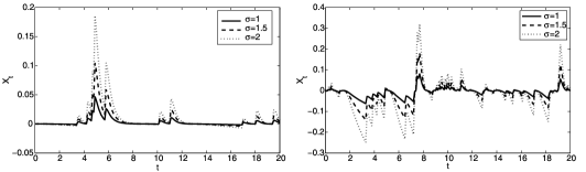
Figure 1: Sample paths of a solution of the Cox–Ingersoll–Ross model (46) with $X_{0}=0$ for varying $\sigma$, fixed $\lambda=2.5$ and $d=0.35$, using two different FLP sample paths, left $\theta=0.5$, right $\theta=2.5$.

A natural non-negative transformation of the FLOUP is given by $Z_{t}:=(\sigma\mathcal{L}_{t}^{d,\lambda})^{2}$ for $t\in\mathbb{R}$ (cf. Figure 2), and, using the chain rule from Theorem A.2 and the existence of all appearing Riemann–Stieltjes integrals, we get

$$\mathrm{d}Z_{t} = 2\sigma^{2}\mathcal{L}^{d,\lambda}_{t}\,\mathrm{d}\mathcal{L}^{d,\lambda}_{t}=-2\lambda\sigma^{2}(\mathcal{L}^{d,\lambda}_{t})^{2}\,\mathrm{d}t+2\sigma^{2}\mathcal{L}^{d,\lambda}_{t}\,\mathrm{d}L^{d}_{t}$$

$$= -2\lambda Z_{t}\,\mathrm{d}t+2\sigma\sqrt{Z_{t}}\,\mathrm{d}L^{d}_{t},\qquad t\in\mathbb{R}.$$

Defining now $\kappa(z):=-2\lambda z$ and $\iota(z):=2\sigma\sqrt{z}$ we have $Z$ as a solution to

$$\mathrm{d}Z_{t}=\kappa(Z_{t})\,\mathrm{d}t+\iota(Z_{t})\,\mathrm{d}L^{d}_{t},\qquad t\in\mathbb{R}.$$

However, the triple $((0,\infty),\kappa,\iota)$ is not strongly proper, because assumption (P2) of Definition 4.1 is violated.

We can now formulate the following general result.

Proposition 5.4.

Let $\mathfrak{L}^{{\lambda/2}}(L^{d},\cdot,\cdot)$ be the Ornstein–Uhlenbeck operator from Definition 3.8. Then for $\tau\in\mathbb{R}$ and $z\geq 0$ the process

$$X_{t}^{\lambda,\tau,z}:=\biggl{(}\frac{\sigma}{2}\mathfrak{L}_{t}^{{\lambda/2}}(L^{d},\tau,z)\biggr{)}^{2},\qquad t\in\mathbb{R},$$

solves the SDEs

$$\mathrm{d}X_{t} = -\lambda X_{t}\,\mathrm{d}t+\sigma\sqrt{|X_{t}|}\,\mathrm{d}L^{d}_{t}$$ (47)

and

$$\mathrm{d}X_{t} = -\lambda X_{t}\,\mathrm{d}t+\sigma\sqrt{X_{t}}\,\mathrm{d}L^{d}_{t},\qquad t\in\mathbb{R}.$$ (48)

In fact, any solution to (48) also solves (47).

This result is not surprising, because Theorem 4.5 does not hold for the SDE (47). However, the reverse is not true: a solution of (47) does not necessarily solve (48), because it can be negative. Also the constant process, $X_{t}:=0$, $t\in\mathbb{R}$, solves both (48) and (47).

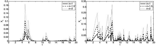
Figure 2: Sample paths of squared FLOUPs for varying $\sigma$, fixed $\lambda=2.5$ and $d=0.35$, using the same sample paths as in Figure 1: left $\theta=0.5$, right $\theta=2.5$.

Considering a squared Ornstein–Uhlenbeck process leads in the case of a driving Brownian motion to a CIR model with mean reversion to positive values. This approach does not work for pathwise integrals, neither in the FLP case nor for FBM, since the Itô term in the chain rule vanishes by finite $p$-variation for some $p<2$.

A positive process based on Theorem 4.4 is given as a solution to

$$\mathrm{d}Y_{t}=-\lambda\sqrt{Y_{t}}\log(Y_{t})\,\mathrm{d}t+\sigma|Y_{t}|\,\mathrm{d}L^{d}_{t},\qquad t\in\mathbb{R},\qquad Y_{0}=y_{0}$$ (49)

for $\lambda,\sigma>0$, cf. Figure 3. Example 5.1 states that the triple for state space $I=(0,\infty)$ is strongly proper and the SST can be calculated as $f(x)=\mathrm{e}^{\sigma x}$.

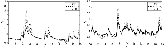
Figure 3: Sample paths of a solution of (49) for varying $\sigma$, fixed $\lambda=2.5$ and $d=0.35$, using the same sample paths as in Figure 1: left $\theta=0.5$, right $\theta=2.5$.

Appendix: Riemann–Stieltjes integration

As mentioned in the Introduction, all integrals in this paper are considered Riemann–Stieltjes integrals, if not stated otherwise. That is, for functions $f,h\mathchoice{\nobreak\,\colon}{\nobreak\,\colon}{\nobreak\,\colon\;}{\nobreak\,\colon\;}[a,b]\mapsto\mathbb{R}$, we take the limit of

$$S(f,g,\kappa,\rho):=\sum_{i=1}^{n}f(y_{i})[h(x_{i})-h(x_{i-1})],$$ (A.1)

where $\kappa=(x_{i})_{i=0,\ldots,n}$ is a partition and $\rho=(y_{i})_{i=1,\ldots,n}$ an intermediate partition of $[a,b]$, that is,

$$a=x_{0}<x_{1}<\cdots<x_{n-1}<x_{n}=b,\qquad x_{i-1}\leq y_{i}\leq x_{i}\qquad\mbox{for all }i\in\{1,\ldots,n\},$$

while letting $\operatorname{\textbf{mesh}}(\kappa):=\sup_{i=1,\ldots,n}|x_{i}-x_{i-1}|$ go to zero. Using the Banach–Steinhaus theorem, one can prove that if for a right-continuous $h$ and all continuous $f$ the Riemann–Stieltjes sums of (A.1) converge, $h$ is already of bounded variation. However, we can weaken this assumption on the integrator by restricting the space of possible integrands. Recall the definitions in (7) and (8). Exploiting the concept of $p$-variation we now state an existence theorem for Riemann–Stieltjes integrals proven by Young [17].

Theorem A.1

Let $[a,b]\subset\mathbb{R}$ be a compact interval, $f\in\mathfrak{W}^{\mathrm{con}}_{q}([a,b])$ and $h\in\mathfrak{W}^{\mathrm{con}}_{p}([a,b])$ for some $p,q>0$ with $p^{-1}+q^{-1}>1$. Then $\int_{a}^{b}f_{s}\,\mathrm{d}h_{s}$ exists in the Riemann–Stieltjes sense.

As in the classical Riemann–Stieltjes calculus, a chain rule can be proven; see [18], Theorem 3.1.

Theorem A.2 ((Chain rule))

Let $[a,b]$ be a compact interval and $g\in\mathfrak{W}^{\mathrm{con}}_{p}([a,b])$ for some $p\in(0,2)$. Furthermore, let $F\in\mathcal{C}^{1}(\mathbb{R})$ with $F^{\prime}\in\operatorname{Lip}(\mathbb{R})$. Then the Riemann–Stieltjes integral $\int_{a}^{b}(F^{\prime}\circ g)_{s}\,\mathrm{d}g_{s}$ exists and we have

$$(F\circ g)(b)-(F\circ g)(a)=\int_{a}^{b}(F^{\prime}\circ g)_{s}\,\mathrm{d}g_{s}.$$ (A.2)

At last we state a density formula, which we have not found in the literature; for a proof we refer to [5], Theorem 4.3.2.

Theorem A.3 ((Density formula))

Let $[a,b]\subset\mathbb{R}$ be a compact interval, $f,h\in\mathfrak{W}^{\mathrm{con}}_{q}([a,b])$ and $g\in\mathfrak{W}^{\mathrm{con}}_{p}([a,b])$ for some $q>0$ and $p>1$ with $p^{-1}+q^{-1}>1$. For all $x\in[a,b]$ we define $\phi(x):=\int_{a}^{x}h_{s}\,\mathrm{d}g_{s}$. Then we have $\phi\in\mathfrak{W}^{\mathrm{con}}_{p}([a,b])$ and

$$\int_{a}^{b}f_{s}\,\mathrm{d}\phi_{s}=\int_{a}^{b}f_{s}h\,\mathrm{d}g_{s}.$$ (A.3)

References

• [1] Buchmann, B. and Klüppelberg, C. (2006). Fractional integral equations and state space transforms. Bernoulli 12 431–456. MR2232725
• [2] Cheridito, P., Kawaguchi, H. and Maejima, M. (2003). Fractional Ornstein–Uhlenbeck processes. Electron. J. Probab. 8 1–14. MR1961165
• [3] Cox, J.C., Ingersoll, J.E. and Ross, S.A. (1985). A theory of term structure of interest rates. Econometrica 53 385–407. MR0785475
• [4] Doss, H. (1977). Liens entre équations différentielles stochastiques et ordinaires. Ann. Inst. Henri Poincaré 13 99–125. MR0451404
• [5] Fink, H. (2008). Fractional Lévy Ornstein–Uhlenbeck processes. Bachelor’s thesis, Technische Universität München.
• [6] Gripenberg, N. and Norros, I. (1996). On the prediction of fractional Brownian motion. J. Appl. Probab. 33 400–410. MR1385349
• [7] Ikeda, N. and Watanabe, S. (1989). Stochastic Differential Equations and Diffusion Processes, 2nd ed. Amsterdam: North-Holland. MR1011252
• [8] Karatzas, I. and Shreve, S.E. (1988). Brownian Motion and Stochastic Calculus. New York: Springer. MR0917065
• [9] Klüppelberg, C. and Matsui, M. (2010). Generalized fractional Lévy processes with fractional Brownian motion limit and applications to stochastic volatility. Available at http://www-m4.ma.tum.de/Papers/index.html. To appear.
• [10] Lyons, T. (1994). Differential equations driven by rough signals (I): An extension of an equality of L.C. Young. Math. Res. Lett. 1 451–464. MR1302388
• [11] Mandelbrot, B.B. and Hudson, R.L. (1968). Fractional Brownian motions, fractional noises and applications. SIAM Rev. 10 422–437. MR0242239
• [12] Marquardt, T. (2006). Fractional Lévy processes with an application to long memory moving average processes. Bernoulli 12 1009–1126. MR2274856
• [13] Samorodnitsky, G. and Taqqu, M. (1994). Stable Non-Gaussian Random Processes: Stochastic Models with Infinite Variance. New York: Chapman & Hall. MR1280932
• [14] Sato, K.-I. (2006). Additive processes and stochastic integrals. Illinois J. Math. 50 825–851. MR2247848
• [15] Sussman, H. (1978). On the gap between deterministic and stochastic ordinary differential equations. Ann. Probab. 6 19–41. MR0461664
• [16] Wheeden, R.L. and Zygmund, A. (1977). Measure and Integral. New York: Marcel Dekker. MR0492146
• [17] Young, L.C. (1936). An inequality of Hölder type, connected with Stieltjes integration. Acta Math 67 251–282. MR1555421
• [18] Zähle, M. (1998). Integration with respect to fractal functions and stochastic calculus I. Probab. Theory Related Fields 111 333–374. MR1640795
• [19] Zähle, M. (2001). Integration with respect to fractal functions and stochastic calculus II. Math. Nachr. 225 145–183. MR1827093