Coherent properties of nano-electromechanical systems

Abstract

We study the properties of a nano-electromechanical system in the coherent regime, where the electronic and vibrational time scales are of the same order. Employing a master equation approach, we obtain the stationary reduced density matrix retaining the coherences between vibrational states. Depending on the system parameters, two regimes are identified, characterized by either ($i$) an effective thermal state with a temperature lower than that of the environment or ($ii$) strong coherent effects. A marked cooling of the vibrational degree of freedom is observed with a suppression of the vibron Fano factor down to sub-Poissonian values and a reduction of the position and momentum quadratures.

I Introduction

Nano-electromechanical systems roukes (NEMS) represent an intriguing class of devices composed of a nano-mechanical resonator coupled to an electronic nanodevice. Several examples of NEMS have been realized, ranging from single oscillating molecules, park to suspended carbon nanotubes sap ; let ; leroy ; lass and suspended nano-cantilevers or nano-beams. knobel ; nanobeams

In all these devices, the coupling between mechanical and electronic degrees of freedom gives rise to peculiar transport phenomena like Franck-Condon blockade, let ; flens ; koch ; mitra negative differential conductance shen ; sap ; zazunov ; cava ; braggio ; cava1 and remarkable noise characteristics. haupt ; koch Along with their outstanding electronic properties, also mechanical ones are of extreme interest. Indeed, owing to the extreme sensitivity of the vibrating part to the spatial motion, NEMS have been proposed as novel detectors in scanning microscopes sid or as ultra-sensitive nano-scales, being able to detect the mass of even few molecules adhering to them. il ; nanoscale In order to successfully employ a NEMS as a precision position detector it is important to reduce its thermal fluctuations, eventually attaining the ultimate goal of cooling it down to its quantum ground state. giazotto Also, ultra-sensitive NEMS position detectors based on peculiar quantum states such as position-squeezed states mandel have been proposed and experimentally realized. hertz

A great variety of NEMS setups have been investigated theoretically. Typically, the electronic part is composed of a semiconducting, koch2 ; mozy ; nocera ; huss ; merlo ; cava3 normal armour ; armour2 ; doiron or superconducting rod2 ; harvey ; rodr2 ; clerk single quantum dot. kou Double-dot setups have been studied as well. ouy ; huss Different models for the coupling between electrons and vibrons have been considered, ranging from the simple Anderson-Holstein (AH) model koch ; koch2 ; pisto ; pisto_c ; rodr ; nocera ; huss ; merlo ; cava3 ; schultz to microscopic models tailored for specific systems, such as suspended carbon nanotubes. izu ; flens2 ; cava2 Also the influence of external dissipative baths galp3 ; galp4 ; cava3 or radiation fields ouy ; rae ; teufel has been analyzed. In the most complex configurations, interesting physical effects have been predicted. For instance, for a nano-mechanical resonator coupled to a microwave cavity, rae ; teufel ; teufel2 to field driven quantum dot rabl or in configurations with double quantum dots, zippilli ; ouy phonon cooling has been found. With radio frequency quantum dots ruskov and a electromagnetic cavity clerk2 squeezing of the vibron position and momentum quadratures has been theoretically predicted.

Even the simple AH model for a single electronic level coupled to an undamped vibrational mode exhibits a rich physics, part of which is still unexplored. Roughly speaking, two regimes have been considered so far, according to the ratio

$$\gamma=\frac{\Gamma_{0}}{\omega_{0}}$$ (1)

between the vibron frequency, $\omega_{0}$, and the average dot-leads electron tunneling rate, $\Gamma_{0}$.

For fast vibrations, $\gamma\ll 1$, every electron tunneling event occurs over many oscillator periods. Then the electrons are not sensitive to the position of the oscillator, but only to its energy. pisto ; boubsi Consequently, the oscillator density matrix becomes close to diagonal in the basis of the energy eigenstates. boubsi Many groups focused their attention on this regime, employing rate equations to study transport phenomena as the Franck-Condon blockade, super-Poissonian shot noise  koch ; mitra ; shen ; koch2 and even peculiar effects such as sub-Poissonian out of equilibrium vibron distributions. rod2 ; merlo ; cava3 ; brandesfano ; brandesfano2

In the opposite regime of slow vibrations $\gamma\gg 1$, electrons are extremely sensitive to the position of the oscillator, which can be treated in a semi-classical approximation. usmani ; armour ; armour2 ; nocera Indeed, Mozyrsky et al. have shown mozy that it is the onset of a semi-classical Langevin dynamics. In this regime the electronic properties of the system have been especially investigated, in particular the current and shot noise mozy in both limits of weak mozy2 and strong electron-vibron coupling. pisto In the latter case, bi-stability and switching have been addressed. galp3 ; galp4 ; galp5 Recently, the classical phase space of the vibron has also been studied. huss

Less attention has been devoted so far to the coherent regime, where the off-diagonal elements of the system density matrix in the energy representation play a relevant role. In this regime, which starts around $\gamma\gtrsim 1$ (for a more precise discussion, see Sec. III.1), the competition between the vibron and the electron time scales gives rise to a tough theoretical problem. Most of the results obtained so far, concerning bi-stability and phase space analysis, have been obtained stretching somehow the validity range of semi-classical approaches, huss ; mozy ; mozy2 in the limit of very low temperatures, $\tau\ll 1$, where

$$\tau=\frac{k_{\mathrm{B}}T}{\hbar\omega_{0}}\,,$$ (2)

here $k_{\mathrm{B}}$ is the Boltzmann constant and $T$ the environment temperature. The interplay of electron and vibron time scales is expected to strongly influence the dynamics of the vibron. For instance, for a NEMS based on a metallic dot in the weak coupling regime, the damping effect of tunneling electrons on the vibron dynamics is maximal when $\omega_{0}\approx\Gamma_{0}$. rodr Similar mechanisms could play a role also in the simpler model of a single level quantum dot.

Motivated by these considerations, in this article we investigate the vibronic properties in the coherent regime $\gamma\gtrsim 1$. Here, because of the off-diagonal structure of the system density matrix, a simple rate equation is no longer justified. blum We derive a generalized master equation brandes1 ; rod ; flindt ; nov ; sch2 in the sequential tunneling regime, in which all off-diagonal elements of the reduced density matrix in the energy eigenbasis are retained. In the limit of high temperatures considered here, $\tau>1$, a fairly large number of basis states have to be included. This fact leads to a serious numerical challenge. Our calculation extends up to $\tau\leq\tau_{\mathrm{max}}$, where $\tau_{\mathrm{max}}\approx 10$. We remark that, as a difference with previous studies, mozy2 our approach is not restricted to small electron-vibron coupling.

Here is a summary of our findings. With the exception of a region $\gamma\to\tau$, in the stationary regime the vibron state can be approximately described in terms of an effective thermal distribution. In the coherent regime, the effective temperature is lower than the environmental temperature. Here, the role of coherences is crucial despite subtle. Non-vanishing off-diagonal elements of the vibron density matrix in the eigenbasis, despite being very small compared with diagonal elements, originate the peculiar effective thermal re-distributions of the vibron occupation probabilities.
When $\gamma\simeq\tau$, the system exhibits deviations from the above effective thermal state. The off-diagonal elements are larger, leading to a marked suppression of the vibron fluctuations even below the Poissonian value. The main results of our paper concern the stationary vibron properties in the coherent regime and can be summarized as follows:
($i$) a cooling of the vibrational mode with respect to the temperature of the electronic environment;
($ii$) a strong suppression of the vibron Fano factor eventually reaching sub-Poissonian values;
($iii$) a reduction of the variances of the vibron position and momentum quadratures.

We remark that the reported cooling phenomenon is a direct consequence of the NEMS entering the coherent regime. It is not “induced” by any external drive or dynamics, like connecting the system to several reservoirs at different temperatures. pisto_c
All the above effects are more pronounced when the electron-vibron coupling strength is increased and none of them comes out treating the system with a simple rate equation involving the diagonal matrix elements only.

The paper is structured as follows. In Sec. II we describe the Anderson-Holstein model and the derivation of the generalized master equation in the stationary regime. In Sec. III we illustrate the coherence effects on the vibron behavior and on the electronic degree of freedom. The large discrepancy with respect to the results obtained by means of a simple rate equation is highlighted. Conclusions are drawn in Sec IV.

II Model and Methods

II.1 Anderson-Holstein Model

In the AH model, flens ; mitra ; koch2 the hamiltonian

$$H=H_{\rm{dot}}+H_{\rm{osc}}+H_{\rm{int}}\,,$$ (3)

describes a ultra-small quantum dot ($H_{\rm{dot}}$) coupled to an harmonic oscillator ($H_{\rm{osc}}$) via the coupling term $H_{\rm{int}}$. The quantum dot is modeled koenig96 as a spin degenerate single level with the average level spacing of the order of the charging energy $E_{\rm{C}}$ (from now on, $\hbar=1$)

$$H_{\rm{dot}}=\epsilon\hat{n}+E_{\mathrm{C}}\hat{n}(\hat{n}-1).$$ (4)

Here, $\hat{n}=\sum_{\sigma=\pm 1}\hat{n}_{\sigma}$ is the occupation number of the level, with $\hat{n}_{\sigma}=d^{{\dagger}}_{\sigma}d_{\sigma}$ the occupation of spin $\sigma/2$ with $\sigma=\pm 1$ and $d_{\sigma}$, $d^{{\dagger}}_{\sigma}$ are the fermionic dot operators. We assume that $E_{\mathrm{C}}$ is the largest energy scale of the problem and we consider only single excess occupancy on the dot, $n=0,1$. The energy $\epsilon=\xi+2E_{\rm{C}}(1/2-n_{\rm{g}})$ includes the energy of the lowest unoccupied single-particle level $\xi$ and a term connected to $n_{\rm{g}}=C_{\rm{g}}V_{\rm{g}}/e$, the charge induced by the gate voltage $V_{\rm{g}}$ with gate capacitance $C_{\rm{g}}$ ($-e$ is the electron charge). cava3

The vibron is described as an harmonic oscillator with mass $m$ and frequency $\omega_{0}$. In terms of the boson operators $b$, $b^{{\dagger}}$ it is modeled as

$$H_{\rm{osc}}=\omega_{0}\left(b^{{\dagger}}b+1/2\right).$$ (5)

The dot and the oscillator are coupled via a term bi-linear in the oscillator position $x$ and in the effective charge number on the dot, $\hat{n}-n_{\rm{g}}$, zazunov ; shen

$$H_{\rm{int}}=\sqrt{2}\lambda\omega_{0}\frac{x}{\ell_{0}}(\hat{n}-n_{\rm{g}})\,,$$ (6)

where $\lambda$ is the adimensional coupling parameter and

$$\ell_{0}=\frac{1}{\sqrt{m\omega_{0}}}$$ (7)

is the characteristic length of the harmonic oscillator.

The dot is coupled also to the external left ($\rm{L}$) and right ($\rm{R}$) leads of non interacting electrons

$$H_{\rm{leads}}=\!\!\!\!\sum_{\alpha=\rm{L},\rm{R}}\sum_{k,\sigma=\pm 1}\varepsilon_{k}\ c^{\dagger}_{\alpha,k,\sigma}c_{\alpha,k,\sigma}\,,$$ (8)

where $c_{\alpha,k,\sigma}$ and $c^{\dagger}_{\alpha,k,\sigma}$ are the fermionic operators. The leads are assumed in equilibrium with respect to their electrochemical potential $\mu_{\rm{L},\rm{R}}=\mu_{0}\pm eV/2$, where $V$ is a symmetrically applied bias voltage, and $\mu_{0}$ is the reference chemical potential. The bias $V$ forces electrons to flow from the left to the right lead through the dot via the tunneling hamiltonian

$$H_{\rm{t}}=t_{0}\sum_{\alpha=\rm{L},\rm{R}}\sum_{k,\sigma=\pm 1}c^{\dagger}_{\alpha,k,\sigma}d_{\sigma}+\rm{h.c.}\,,$$ (9)

where $t_{0}$ is the tunneling amplitude through both the left and right barriers.

Equation (3) can be diagonalized by the Lang–Firsov polaron transformation, zazunov with generator

$$\mathcal{U}=\exp{[\hat{\eta}\,(b^{\dagger}-b)]}\quad\mbox{and}\quad\hat{\eta}=\lambda\,(\hat{n}-n_{\rm{g}}).$$ (10)

This procedure imposes no restriction on the possible values of $\lambda$. The transformed operators in the polaron frame $\bar{\mathcal{O}}=\mathcal{U}\mathcal{O}\mathcal{U}^{\dagger}$ are $\bar{b}=b-\hat{\eta}$ and $\bar{d}_{\sigma}=d_{\sigma}\exp{\left[\lambda(b-b^{\dagger})\right]}$, while $\hat{n}$ is invariant. The diagonal Hamiltonian, expressed in terms of the original operators reads

$$\bar{H}=\bar{\epsilon}\,\hat{n}+\omega_{0}(b^{{\dagger}}b+1/2)\ ,$$ (11)

with renormalized level position $\bar{\epsilon}=\xi+(E_{\mathrm{C}}-\lambda^{2}\omega_{0})(1-2n_{\mathrm{g}})$. In the following we choose $\mu_{0}=\xi$ setting the resonance between the $n=0,1$ states at $n_{\rm{g}}=1/2$. The eigenstates of Eq. (11) will be denoted as $|n,l\rangle$, where $n$ is the dot occupation number and $l$ represents the vibron number. The transformed tunneling Hamiltonian is

$$\bar{H}_{\rm{t}}=t_{0}\sum_{\alpha=\rm{L},\rm{R}}\sum_{k,\sigma=\pm 1}e^{\lambda(b-b^{\dagger})}c^{\dagger}_{\alpha,k,\sigma}d_{\sigma}+\rm{h.c.}\,.$$ (12)

II.2 Master Equation

The dynamics of the dot and the oscillator is described by the reduced density matrix ${\bar{\rho}}(t)$, defined as the trace over the leads of the total density matrix $\bar{\rho}_{\rm{tot}}(t)$, in the polaron frame

$$\bar{\rho}(t)=\mathrm{Tr}_{\rm{leads}}\{{\bar{\rho}}_{\rm{tot}}(t)\}\,.$$ (13)

We consider the sequential, weak tunneling regime, treating $\bar{H}_{\rm{t}}$ in Eq. (12) to the lowest order. This approximation is valid for not too low temperatures $T$, $\Gamma_{0}=2\pi|t_{0}|^{2}\nu<k_{\rm{B}}T$, where $\nu$ is the leads density of states. We further perform the Born approximation, timm assuming that the system and the leads are independent before $H_{\mathrm{t}}$ is switched on. This amounts to take the factorized form at $t=0$, $\bar{\rho}_{\rm{tot}}(0)=\bar{\rho}(0)\otimes\rho_{\rm{l}}(0)$, where $\rho_{\rm{l}}(0)=\rho_{\rm{L}}(0)\otimes\rho_{\rm{R}}(0)$ and $\rho_{\rm{L/R}}(0)$ are the initial equilibrium density matrices of the left and the right lead respectively.

In the interaction picture with respect to $\bar{H}_{\rm{t}}$, any operator, $A$, is transformed as

$$A_{\rm{I}}=e^{i(\bar{H}+H_{\rm{leads}})t}Ae^{-i(\bar{H}+H_{\rm{leads}})t}.$$

The reduced density matrix evolves according to

$$\begin{split}\!\!\!\!\!\dot{\bar{\rho}}_{\rm{I}}(t)&\!\!=\!-\!\!\!\!\sum_{\sigma=\pm 1}\!\int_{0}^{t}\!\!{\rm d}t^{\prime}\!\left\{\![Q_{\rm{I},\sigma}(t),Q^{\dagger}_{\rm{I},\sigma}(t^{\prime})\bar{\rho}_{\mathrm{I}}(t^{\prime})]K^{+}(t-t^{\prime})\right.\\ &-[Q_{\rm{I},\sigma}(t),\bar{\rho}_{\rm{I}}(t^{\prime})Q^{\dagger}_{\rm{I},\sigma}(t^{\prime})]K^{-}(t^{\prime}-t)\\ &+[Q^{\dagger}_{\rm{I},\sigma}(t),Q_{\rm{I},\sigma}(t^{\prime})\bar{\rho}_{\rm{I}}(t^{\prime})]K^{-}(t-t^{\prime})\\ &-\left.[Q^{\dagger}_{\rm{I},\sigma}(t),\bar{\rho}_{\rm{I}}(t^{\prime})Q_{\rm{I},\sigma}(t^{\prime})]K^{+}(t^{\prime}-t)\right\}\,.\end{split}$$ (14)

Here,

$$Q_{\rm{I},\sigma}(t)=e^{\lambda(b_{\rm{I}}(t)-b_{\rm{I}}^{\dagger}(t))}d_{\rm{I},\sigma}(t)\,,$$

and $K^{\pm}(t)=K_{\mathrm{L}}^{\pm}(t)+K_{\mathrm{R}}^{\pm}(t)$ are the leads correlation functions

$$\begin{split}K_{\alpha}^{+}(t)&=|t_{0}|^{2}\sum_{k}\mathrm{Tr}_{\mathrm{leads}}\left\{c^{{\dagger}}_{\alpha,k,\sigma}(t)c_{\alpha,k,\sigma}(0)\rho_{\rm{l}}\right\},\\ K_{\alpha}^{-}(t)&=|t_{0}|^{2}\sum_{k}\mathrm{Tr}_{\mathrm{leads}}\left\{c_{\alpha,k,\sigma}(t)c_{\alpha,k,\sigma}^{{\dagger}}(0)\rho_{\rm{l}}\right\}\,.\\ \end{split}$$ (15)

In Eq. (14) we performed the large reservoirs approximation timm

$$\bar{\rho}_{\mathrm{I,tot}}(t^{\prime})=\bar{\rho}_{\mathrm{I}}(t^{\prime})\cdot\rho_{l}$$ (16)

assuming that tunneling events have a negligible effect on the leads, which remain in the thermal equilibrium state, denoted as $\rho_{\rm{l}}$. In the weak tunneling regime ($\Gamma_{0}<k_{\rm{B}}T$) one can replace $\bar{\rho}_{\mathrm{I}}(t^{\prime})\approx\bar{\rho}_{\mathrm{I}}(t)$ using the standard Markov approximation, and extend the integration limit to $\infty$.

Eq. (14) can be projected on the eingenstates of the hamiltonian (11), obtaining an infinite set of coupled equations for the density matrix elements $\langle n,l|\bar{\rho}(t)|n^{\prime},l^{\prime}\rangle$ (where $n,n^{\prime}\in\{0,1\}$ and $l,l^{\prime}\geq 0$). It can be easily shown that diagonal and off-diagonal elements in the electron number decouple and in the stationary regime the latter tend to zero. In fact, the coupling of the leads and the dot charge leads to a rapid decay of superpositions of dot states with different charges. gurv ; timm Since we are interested in the stationary properties, we focus on the density matrix elements diagonal in the electron level occupation number, $\bar{\rho}_{qq^{\prime}}^{n}(t)=\langle n,q|\bar{\rho}(t)|n,q^{\prime}\rangle$. They obey the following generalized master equation (GME)

$$\dot{\bar{\rho}}_{\mathrm{I},qq^{\prime}}^{n}(t)=\sum_{pp^{\prime}n^{\prime}}\mathcal{R}_{qq^{\prime}pp^{\prime}}^{nn^{\prime}}e^{i\omega_{0}(q-q^{\prime}-p+p^{\prime})t}\;\,\bar{\rho}^{n^{\prime}}_{\mathrm{I},pp^{\prime}}(t)\,,$$ (17)

where $\mathcal{R}_{qq^{\prime}pp^{\prime}}^{nn^{\prime}}$ are the Redfield tensor elements blum

$$\begin{split}\mathcal{R}_{qq^{\prime}pp^{\prime}}^{01}=&X_{qp}X_{q^{\prime}p^{\prime}}\left[C^{-}(\omega_{pq})^{*}+C^{-}(\omega_{p^{\prime}q^{\prime}})\right]\,,\\ \mathcal{R}_{qq^{\prime}pp^{\prime}}^{11}=&-\sum_{l}\left[X_{lq^{\prime}}X_{lp^{\prime}}C^{-}(\omega_{p^{\prime}l})\delta_{pq}\right.\\ &\left.+X_{lq}X_{lp}C^{-}(\omega_{pl})^{*}\delta_{p^{\prime}q^{\prime}}\right]\,,\end{split}$$ (18)

$$\begin{split}\mathcal{R}_{qq^{\prime}pp^{\prime}}^{10}=&2X_{pq}X_{p^{\prime}q^{\prime}}\left[C^{+}(\omega_{qp})+C^{+}(\omega_{q^{\prime}p^{\prime}})^{*}\right]\,,\\ \mathcal{R}_{qq^{\prime}pp^{\prime}}^{00}=&-2\sum_{l}\left[X_{q^{\prime}l}X_{p^{\prime}l}C^{+}(\omega_{lp^{\prime}})^{*}\delta_{pq}\right.\\ &\left.+X_{ql}X_{pl}C^{+}(\omega_{lp})\delta_{p^{\prime}q^{\prime}}\right]\,.\end{split}$$ (19)

Here $\omega_{qq^{\prime}}\equiv\omega_{0}(q-q^{\prime})$ and

$$\begin{split}X_{qq^{\prime}}&=\langle q|e^{\lambda(b-b^{{\dagger}})}|q^{\prime}\rangle\\ &=e^{-\frac{\lambda^{2}}{2}}\sqrt{\frac{q_{<}!}{q_{>}!}}L^{|q^{\prime}-q|}_{q_{<}}(\lambda^{2})\left[\mathrm{sgn}(q^{\prime}-q)\lambda\right]^{|q^{\prime}-q|}\,,\\ \end{split}$$ (20)

are the generalized Franck-Condon factors koch ; cava3 , with $q_{<}=\min\left\{q,q^{\prime}\right\}$, $q_{>}=\max\left\{q,q^{\prime}\right\}$ and $L^{n}_{q}(x)$ the generalized Laguerre polynomials. abra The factors 2 in Eqs. (19) are due to the spin degeneracy. In Eqs. (18),(19) the generalized tunneling rates $C^{\pm}(\omega_{qq^{\prime}})=C_{\mathrm{L}}^{\pm}(\omega_{qq^{\prime}})+C_{\mathrm{R}}^{\pm}(\omega_{qq^{\prime}})$ have also been introduced

$$C^{\pm}_{\alpha}(\omega_{qq^{\prime}})=\int_{0}^{\infty}\mathrm{d}\theta K^{\pm}_{\alpha}(\pm\theta)e^{-i(\bar{\epsilon}+\omega_{qq^{\prime}})\theta}\,.$$ (21)

Exploiting the identity

$$\int_{0}^{\infty}\mathrm{d}\theta\exp{\left(i\Omega\theta\right)}=\pi\delta(\Omega)+iP.V.(1/\Omega)\,,$$

and the explicit form of the leads correlation function scholler

$$K^{\pm}_{\alpha}(t)={-}\frac{i\Gamma_{0}e^{\pm i\mu_{\alpha}t}}{2\beta\sinh{[\frac{\pi}{\beta}(t-\frac{i}{\omega_{\rm{c}}})]}}\,,\\$$

with $\omega_{\rm{c}}$ the cut-off energy and $\beta=1/(k_{\rm{B}}T)$, one has

$$C^{\pm}(\omega_{qq^{\prime}})=\frac{\Gamma_{0}}{2}\sum_{\alpha}\left[f_{\alpha}^{\pm}(\omega_{qq^{\prime}})\pm i\Delta_{\alpha}(\omega_{qq^{\prime}})\right]\,.$$ (22)

Here

$$f_{\alpha}^{+}(E)=\frac{1}{1+e^{\beta(\bar{\epsilon}+E-\mu_{\alpha})}}$$ (23)

is a Fermi function, $f^{-}_{\alpha}(E)=1-f^{+}_{\alpha}(E)$ and

$$\Delta_{\alpha}(\omega_{qq^{\prime}})=\log\left(\frac{2\pi}{\beta\omega_{\mathrm{c}}}\right)+\mathrm{Re}\,\psi\left[\frac{1}{2}+\frac{i\beta}{2\pi}(\bar{\epsilon}+\omega_{qq^{\prime}}-\mu_{\alpha})\right]$$

the depolarization shift. The stationary system properties are obtained from the solution of the steady-state GME

$$\sum_{pp^{\prime}n^{\prime}}\left[\mathcal{R}_{qq^{\prime}pp^{\prime}}^{nn^{\prime}}+i\omega_{0}\left(p^{\prime}-p\right)\delta_{pq}\delta_{p^{\prime}q^{\prime}}\right]\bar{\rho}^{n^{\prime}}_{pp^{\prime}}=0\,,$$ (24)

written here in the Schrödinger representation, for the stationary values of the reduced density matrix elements

$$\bar{\rho}_{pp^{\prime}}^{n}=\lim_{t\to\infty}\bar{\rho}_{pp^{\prime}}^{n}(t)\,.$$ (25)

Note that the GME (24) takes into account both all off-diagonal (coherences) and diagonal terms in the vibron number.
The steady state current calculated e.g. on the right tunnel barrier, reads

$$I=e\Gamma_{0} \sum_{pqq^{\prime}}\left\{-2\left[C^{+}_{\mathrm{R}}(\omega_{pq^{\prime}})+C^{+}_{\mathrm{R}}(\omega_{pq})^{*}\right]X_{qp}X_{q^{\prime}p}\bar{\rho}_{qq^{\prime}}^{0}\right.$$ (26)

$$+\left.\left[C^{-}_{\mathrm{R}}(\omega_{qp})+C^{-}_{\mathrm{R}}(\omega_{q^{\prime}p})^{*}\right]X_{pq}X_{pq^{\prime}}\bar{\rho}_{qq^{\prime}}^{1}\right\}\,.$$

Note that in the steady-state the current is independent of the barrier index.

II.3 Rotating Wave Approximation

In the regime of fast vibrational motion, $\gamma\ll 1$, the contribution of fast oscillatory terms to the solution of Eq. (17) is negligible. It is then possible to perform the rotating wave approximation (RWA), neglecting the oscillating contributions and including only the dominant secular terms. blum They are those which connect density matrix elements with $p-p^{\prime}=q-q^{\prime}$. This implies that the diagonal elements $\bar{\rho}_{qq}^{n}$ are decoupled from the off-diagonal ones $\bar{\rho}_{pp^{\prime}}^{n}$ with $p^{\prime}\neq p$. In addition, the non-diagonal elements vanish in the stationary regime. mitra Hence stationary properties are fully described by the diagonal occupation probabilities $\bar{P}_{nq}=\bar{\rho}^{n}_{qq}$ and Eq. (24) reduces to a standard rate equation

$$z_{n}\bar{P}_{nq}\sum_{n^{\prime}\neq n}\sum_{p=0}^{\infty}\Gamma_{qp}^{nn^{\prime}}-\sum_{n^{\prime}\neq n}\sum_{p=0}^{\infty}z_{n^{\prime}}\bar{P}_{n^{\prime}p}\Gamma_{pq}^{n^{\prime}n}=0\,.$$ (27)

The coefficients $z_{n}$ stem from the spin degeneracy: $z_{0}=2$, $z_{1}=1$. The tunneling rates $\Gamma_{pq}^{nn^{\prime}}=\Gamma_{{\mathrm{L}},pq}^{nn^{\prime}}+\Gamma_{\mathrm{R},pq}^{nn^{\prime}}$ for the transition $|n,p\rangle\rightarrow|n^{\prime},q\rangle$, are

$$\begin{split}\!\!\!\!\Gamma_{\alpha,qp}^{nn+1}=&\,2X_{pq}^{2}\mathrm{Re}\left\{C_{\alpha}^{+}(\omega_{pq})\right\}\!=\!\Gamma_{0}X_{pq}^{2}f^{+}_{\alpha}(\omega_{pq});\\ \!\!\!\!\Gamma_{\alpha,pq}^{n+1n}=&\,2X_{pq}^{2}\mathrm{Re}\left\{C_{\alpha}^{-}(\omega_{pq})\right\}\!=\!\Gamma_{0}X_{pq}^{2}f^{-}_{\alpha}(\omega_{pq}).\end{split}$$ (28)

Note that Eq. (27) does not depend on $\gamma$.
Within the RWA, the steady-state current Eq. (26) is

$$I_{\rm{RWA}}=e\Gamma_{0}\sum_{p,q}\left[-2\bar{P}_{0q}\Gamma_{\mathrm{R},qp}^{0,1}+\bar{P}_{1q}\Gamma_{\mathrm{R},qp}^{1,0}\right]\,.$$ (29)

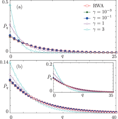
Figure 1: (Color online) Vibron occupation probabilities $\bar{P}_{q}$ as a function of the vibron number $q$, calculated numerically solving the RWA rate equation in Eq. (27) (red empty squares) and the GME in Eq. (24). Here $\gamma=3$ (cyan empty triangles), $\gamma=1$ (purple empty circles), $\gamma=10^{-1}$ (blue circles), $\gamma=10^{-3}$ (green squares). (a) $\lambda=0.5$ and $eV=\omega_{0}$. (b) Main panel: $\lambda=0.5$ and $eV=20\,\omega_{0}$. Inset: $\lambda=2$ and $eV=20\,\omega_{0}$. In all panels other parameters are $\tau=6$, $n_{\rm{g}}=1/2$ and $\omega_{\rm{c}}=10^{6}\,\omega_{0}$.

Results presented in the following Section are obtained by numerical solution of the GME Eq. (24) truncating the size of the vibron Hilbert space until convergence is reached (see next Section for details). In the limit $\gamma\ll 1$, this approach accurately reproduces the well-known solution of the RWA rate equation. rodr ; pisto_c ; merlo ; koch ; koch2

This is illustrated in Fig. 1, where the diagonal elements of the reduced density matrix, $\bar{P}_{q}=\sum_{n}\bar{\rho}^{n}_{qq}$, obtained by solving the GME for different values of $\gamma$ are shown. The solutions of the GME converge to those in the RWA for $\gamma\rightarrow 0$ (red squares), both for small and large voltages (panels (a) - (b)) and even in the strong electron-vibron coupling regime (panel c). This convergence has been systematically observed in the whole range of parameters and constitutes a validation of our numerical procedure.
On the other hand, with increasing $\gamma$, deviations from the RWA are obtained. They are originated from the coherent off-diagonal elements of $\bar{\rho}_{qq^{\prime}}$. These deviations represent the central part of our work and relevant consequences will be discussed in details in the following Section.

III Results

In the present Section, we investigate the stationary equilibrium properties of the system as a function of the parameters $\gamma$, $\tau$ defined in Eqs.(1), (2). Here, $\gamma$ distinguishes between fast, slow or coherent regimes, and $\tau$ is the reduced temperature. We focus mainly on the vibronic properties. Relevant quantities of our interest are the vibron Fano factor and the position and momentum quadratures. Their behavior can be understood by first analyzing the structure of the oscillator density matrix in the vibron eigenbasis. In the final part of this Section, the electronic current and the average electronic occupation of the dot will be briefly addressed.

III.1 Parameters regimes

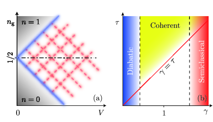
Figure 2: (Color online) (a) Stability diagram in the $(V,n_{\mathrm{g}})$ plane: gray shaded regions denotes Coulomb Blockade regime. Blue (solid) lines mark the onset of transitions between ground states, red (dashed) lines signal transitions involving excited states of the vibron. (b) Different regimes as a function of $\gamma=\Gamma_{0}/\omega_{0}$ and $\tau=k_{\mathrm{B}}T/\omega_{0}$. The blue shaded region denotes the “diabatic” regime of fast vibrations, the red one the semi-classical regime with $\omega_{0}\ll\Gamma_{0}$. The region above the line $\gamma=\tau$ marks the region accessible by our methods and the yellow shaded area indicates the accessible regime where coherences among vibron states become important.

Figure 2(a) represents the stability diagram of the system as a function of the bias voltage $V$ and of $n_{\mathrm{g}}$. In the shaded (gray) regions the system is in the Coulomb blockade regime with the dot empty (full) if $n_{\mathrm{g}}<1/2$ ($n_{\mathrm{g}}>1/2$). The blue (solid) lines mark transitions between the states $|0,q\rangle$ and $|1,q\rangle$ ($n$ and $q$ are the occupation number of the electronic or vibronic states $|n,q\rangle$). Red (dashed) lines indicate the activation threshold for transport channels with transitions $|n,q\rangle\to|n^{\prime},q^{\prime}\rangle$ where in general $q,q^{\prime}\neq 0$. The boundaries of different transport regions are thermally broadened.
In the following analysis we will focus at $n_{\mathrm{g}}=1/2$ where the $n=0$ and $n=1$ charge states are on resonance (dashed-dotted line in Fig. 2(a)). Qualitatively similar results are observed also off-resonance at $n_{\mathrm{g}}\neq 1/2$.
In Fig. 2(b) we report a sketch of the system behavior in the $(\gamma,\tau)$ plane.

We distinguish a “diabatic” regime of fast vibrations for $\gamma\ll 1$ (blue shaded region), where the RWA is valid, rodr ; pisto_c ; merlo ; koch ; koch2 and an “adiabatic” regime of slow vibrations $\gamma\gg 1$ where semiclassical methods have been applied huss ; nocera ; pisto ; galp4 ; mozy with approaches confined to low temperatures $\tau\ll 1$.
The regime in between these two regions is, on the other hand, unexplored. Our GME method fills in precisely this gap. Indeed, we will show that, increasing $\gamma$ from the diabatic regime, marked deviations from the solution of the RWA rate equations appear. Here, coherences represented by the off-diagonal elements of the reduced density matrix are relevant. The constraints on our GME method are:
($i$) the sequential tunneling approximation which implies $0<\gamma<\tau$ (the area above the red line in Fig. 2);
($ii$) a restriction on the temperature $\tau<\tau_{\mathrm{max}}\approx 10$, due to the rapid increase with $\tau$ of the number of vibron states needed for the convergence of our numerical calculations.
Because of these constraints, the transition towards the semiclassical limit cannot be explored.

We solve numerically the GME in the steady state, increasing the size of the vibron Hilbert space including up to 150 oscillator states per charge state in the basis, until convergence is reached. The limitation on the number of oscillator states employed in the calculation is essentially due to computer memory requirements and by the decreasing rate of convergence. At high temperature $\tau\approx 10$, already more than 100 oscillator basis states are required for convergence.

III.2 Overview of the results

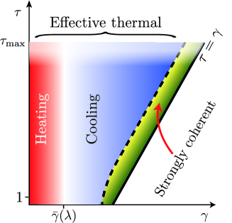
Figure 3: (Color online) Schematic overview of the results in the $(\gamma,\tau)$ plane, see text for details on the notation.

Before entering our analysis, we summarise in Fig. 3 the stationary vibronic characteristics we obtain in the various parameter regimes. We address the temperature regime $1\lesssim\tau\lesssim\tau_{\mathrm{max}}$ and $0<\gamma\lesssim\tau$. We will show that in a large parameters range (shaded area) the vibron density matrix

$$\bar{\rho}_{qq^{\prime}}=\sum_{n=0,1}\bar{\rho}_{qq^{\prime}}^{n}$$ (30)

is well approximated by an effective thermal distribution with temperature $\tau_{\rm{eff}}$

$$\bar{\rho}_{qq^{\prime}}^{({\mathrm{th}})}(\tau_{\mathrm{eff}})=\left(1-e^{-1/\tau_{\mathrm{eff}}}\right)e^{-q/\tau_{\mathrm{eff}}}\delta_{q,q^{\prime}}\,.$$ (31)

For $\gamma\ll 1$ the off-diagonal elements of the reduced density matrix are negligible and a fit of $\bar{\rho}_{qq^{\prime}}$ to Eq. (31) leads to $\tau_{\mathrm{eff}}\geq\tau$. This ”heating” phenomenon is due to the finite voltage, and for $V\to 0$ the system attains a thermal equilibrium distribution in the polaron frame, $\tau_{\mathrm{eff}}\to\tau$, as reported in Ref. merlo, .
With increasing $\gamma$ the off-diagonal elements of $\bar{\rho}_{qq^{\prime}}$ increase. The onset of this coherent regime is marked by the condition $\gamma\gtrsim\bar{\gamma}(\lambda)$, with the latter a $\lambda$-dependent threshold value. For typical values $\lambda\approx 1$ we find $0.1\leq\bar{\gamma}(\lambda)\leq 1$. When $\bar{\gamma}(\lambda)\lesssim\gamma<\tau$ the coherences are much smaller than the diagonal elements of the reduced density matrix. In this weakly coherent regime the vibron density matrix can still be fitted with a thermal distribution, but at a lower effective temperature, eventually reaching the cooling regime where $\tau_{\mathrm{eff}}<\tau$. The cooling is always accompanied by a reduction both of the fluctuations of the vibronic population and of the variance of position and momentum quadratures.
A completely different system behavior takes place when $\gamma\to\tau$, (yellow-green area delimited by the dashed and continuous lines in Fig. 3). In this strongly coherent regime off-diagonal terms of the density matrix are paramount and the diagonal part of the density matrix deviates from the simple thermal distribution. Here, despite of the high temperature ($\tau>1$), a non-classical system behavior comes out. Suppression of the vibron populations fluctuations and of the variances of the position and momentum quadratures persists also in this regime.

III.3 Density matrix and cooling

We start our analysis investigating the structure of the oscillator density matrix in the vibron eigenbasis in the regimes indicated in Fig. 3.
We first concentrate on the density matrix $\bar{\rho}_{qq^{\prime}}$ when it is well described by the effective thermal distribution, Eq. (31). In Figs. 4(a) - (b) we report the density plots of $|\bar{\rho}_{qq^{\prime}}|$ in the diabatic and in the coherent regime respectively.

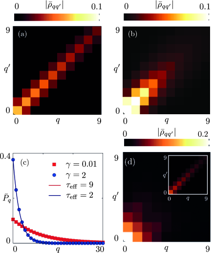
Figure 4: (Color online) Density plot of $|\bar{\rho}_{qq^{\prime}}|$ as a function of $q,q^{\prime}$. Panel (a): $\gamma=0.01$ and $\tau=9$; Panel (b): $\gamma=2$ and $\tau=9$. Panel (c): Occupation probabilities $\bar{P}_{q}=\bar{\rho}_{qq}$ for $\tau=9$ and $\gamma=0.01$ (squares) or $\gamma=2$ (dots). Lines are fit to a thermal distribution with effective temperature $\tau_{\mathrm{eff}}$. In panel (d) $\gamma=1.2$ and $\tau=3$ (main), and $\tau=9$ (inset). In all panels, $n_{\rm{g}}=1/2$, $eV=\omega_{0}$, $\lambda=2$ and $\omega_{c}=10^{6}\ \omega_{0}$.

For $\gamma\ll 1$ - panel (a) - the density matrix is strongly peaked around the diagonal, $q\approx q^{\prime}$. The corresponding occupation probability distribution $\bar{P}_{q}=\bar{\rho}_{qq}$ extends over more than fifteen states Fig. 4(c) (squares). We then perform a numerical fit of $\bar{\rho}_{qq^{\prime}}$ on a thermal distribution in Eq. (31). The fit leads to an effective temperature $\tau_{\mathrm{e}ff}$ with an error $\Delta\tau$, signaling the departure from the approximatively diagonal thermal density matrix. In considered diabatic regime, $\gamma\ll 1$, $\tau_{\mathrm{eff}}\approx\tau$ with a very small relative error $\delta\tau=\Delta\tau/\tau_{\mathrm{eff}}<10^{-4}$.
Increasing $\gamma$, the coherent regime is entered, with a vibron occupation probability considerably altered, see Fig. 4(b). We observe two main modifications. First, off-diagonal elements are larger than in the diabatic regime, even though they remain rather small in comparison with the diagonal ones. Second, the probability distribution along the diagonal gets narrower. Remarkably, the occupation probabilities $\bar{P}_{q}$ are still approximated by a quasi-thermal state but with an effective temperature $\tau_{\mathrm{eff}}$ lower than the environmental one, see Fig. 4(c) circles. The relative error is still rather small, $\delta\tau\approx 6\cdot 10^{-3}$. We remark that this result is a consequence of the non-vanishing vibronic coherences, in fact in the RWA the density matrix would be strictly diagonal, as a difference with Fig. 4(b).

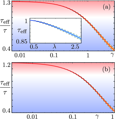
Figure 5: (Color online) Solid lines: effective temperature $\tau_{\mathrm{eff}}$ as a function of $\gamma$, extracted from a numerical fit of $\bar{\rho}_{qq^{\prime}}$ on Eq. (31), (see text). Panel (a): $\tau=9$ and $eV=20\,\omega_{0}$. In the inset $\tau_{\mathrm{eff}}$ as a function of $\lambda$ for $\gamma=6$. Panel (b): $\tau=3$ and $eV=6\,\omega_{0}$. In all panels, dashed lines around the solid line delimit the absolute error on the effective temperature, $\Delta\tau$. Red (blue) gradient areas signal heating (cooling). Other parameters are $n_{\rm{g}}=1/2$ and $\omega_{\rm{c}}=10^{6}\ \omega_{0}$.

The crossover from heating to cooling with increasing $\gamma$ and the accuracy of the thermal approximation measured by the error of the fitting procedure are analyzed in Fig. 5(a) - (b). The absolute error is represented by the shaded area around the continuous line limited by dashed lines. Two different regimes are clearly identified. In the diabatic regime, the effective temperature is larger than that of the environment (red shaded region) and the system exhibits heating. The values of $\tau_{\mathrm{eff}}\geq\tau$ are due to the considered high voltage bias and indeed for $V\to 0$ one obtains $\tau_{\mathrm{eff}}\to\tau$.
As $\gamma$ is increased, cooling occurs (blue shaded region) and $\tau_{\mathrm{eff}}$ drops markedly below the electronic temperature $\tau$. Even though $\tau_{\mathrm{eff}}$ increases for increasing $V$ (not shown) this cooling effect survives up to $eV\approx 20\,\omega_{0}$. It can be seen that the error grows with increasing $\gamma$, signaling the rise of the off-diagonal terms of the density matrix. We can then safely identify the cooling phenomenon provided $\gamma$ does not approach $\tau$. In the inset of Fig 5(a) the typical behavior of $\tau_{\mathrm{eff}}$ as a function of $\lambda$ is shown, with an error on $\tau_{\mathrm{eff}}$ which increases increasing $\lambda$.
We remark that the cooling phenomenon is entirely due to the coherent dynamics of the vibron-electronic system and is not induced by any ad-hoc mechanism acting on the system.

The description in terms of an effective thermal distribution ceases to be valid when $\gamma\to\tau$, as shown by the increasing errors in Fig. 5. To investigate this regime, we consider the case $\tau=3$, $\gamma=1.2$ in Fig. 4(d). Here, although an effective temperature $\tau_{\mathrm{eff}}\approx 0.8<\tau$ can be formally extracted with the fitting procedure, the relative error becomes large $\delta\tau\approx 0.11$. The main source of error are the rather large off-diagonal matrix elements. This is a general trend which we always observed when $\gamma$ approaches $\tau$. As an illustration, we report in the inset of Fig. 4(c) the density matrix for the same parameters of the main panel but at higher temperature ($\tau\gg\gamma$). In this case off-diagonal elements are strongly suppressed and an effective thermal description is then appropriate.
We conclude this paragraph commenting on the dependence of the above results on the electron-vibron coupling strength, $\lambda$, which is not limited in our approach. In Figure 6 (a) - (d) we report the density plot of $|\bar{\rho}_{qq^{\prime}}|$ at fixed $\tau$ and for increasing values of $\lambda$. Increasing the dot-vibron coupling induces an hybridization of the electronic and mechanical degrees of freedom which manifests itself also in the off-diagonal elements of the vibron density matrix between Fock states. Indeed, with increasing $\lambda$ a “delocalization” phenomenon is induced, the density matrix spreading away from the diagonal.

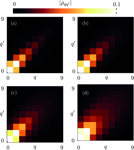
Figure 6: (Color online) Density plot of $|\bar{\rho}_{qq^{\prime}}|$ as a function of $q,q^{\prime}$ for fixed $\gamma$, $\tau$ and different values of the electron-vibron coupling strength. Panel (a): $\lambda=1$; Panel (b): $\lambda=1.5$; Panel (c): $\lambda=2$; Panel (d): $\lambda=2.5$. In all panels, $n_{\rm{g}}=1/2$, $eV=\omega_{0}$, $\gamma=3$, $\tau=6$ and $\omega_{c}=10^{6}\ \omega_{0}$.

III.4 Wigner function and quadratures

Further insight on the system behavior is obtained from the Wigner quasi-probability distribution function mandel

$$W(x,p)=\frac{1}{\pi}\int_{-\infty}^{\infty}{\mathrm{d}}y\ e^{2ipy}\langle x-y|\mathcal{U}^{\dagger}\bar{\rho}\mathcal{U}|x+y\rangle\,,$$ (32)

the quantum analogue of the Liouville density in classical phase space with $\mathcal{U}$ defined in Eq. (10). The Wigner function allows the detection of non-classical features signaled by regions in the $(x,p)$ plane where $W(x,p)<0$. mandel

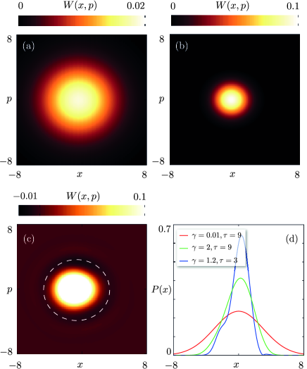
Figure 7: (Color online) Panels (a) - (c) density plot of the Wigner function $W(x,p)$ as a function of $x,p$. In panels (a) and (b) $\tau=9$, and in (a) $\gamma=0.01$, in (b) $\gamma=2$. Note the different color scale in the two panels. (c) Density plot of $W(x,p)$ for $\tau=3$ and $\gamma=1.15$. (d) Probability density of the oscillator position $P(x)$. In all panels $x$ and $p$ are expressed in unity of $\ell_{0}$ and $\ell_{0}^{-1}$ respectively - see Eq. (7). In addition $n_{\rm{g}}=1/2$, $eV=\omega_{0}$, $\lambda=2$ and $\omega_{c}=10^{6}\ \omega_{0}$.

Figures 7(a) - (b) show $W(x,p)$ for the parameters of Figs. 4(a) - (b), in the effective thermal regime. The Wigner functions are positive and can be regarded as the probability density of the oscillator states in the $(x,p)$ phase space. Consistently, their shape closely resembles that of a thermal state, mandel but with a decreased width $\tau_{\mathrm{eff}}$. The shrinkage of $W(x,p)$ observed when entering the coherent regime can be traced back to the role of coherences which mediate the redistribution of the $\bar{P}_{q}$ and the ensuing reduction of $\tau_{\mathrm{eff}}$.
Figure 7(c) shows $W(x,p)$ for $\gamma=1.2$ and $\tau=3$ in the strongly coherent regime, when the system can no longer be described by a thermal distribution (as in Fig. 4(d)). In this case, the width of $W(x,p)$ is still reduced. As a difference with previous case, here we observe that $W(x,p)$ becomes negative in an approximately circular area around the main peak (white dashed circle). This fact signals a non-classical behavior of the system entirely due to the non-diagonal structure of the reduced density matrix. Negative values of $W(x,p)$ are a trademark of the regime $\gamma/\tau\approx 1$. This quantum behavior, naively unexpected at the considered high temperatures $\tau\gtrsim 1$, is a relevant result whose implications on the vibronic fluctuations will be discussed in the next subsection.
Also noteworthy is the elongated shape of $W(x,p)$ along the $x$ direction, Fig. 7(c). This is reflected in the position probability distribution

$$P(x)=\int_{-\infty}^{\infty}{\mathrm{d}}p\ W(x,p)$$ (33)

shown in Figure 7(d). While in the effective-thermal regime $P(x)$ exhibits a single peak, in the regime of strong coherences it shows a peculiar shoulder structure. In this latter regime, for relatively slow tunneling events $\gamma\sim 1$, the oscillator adjusts itself to the two equilibrium positions corresponding to zero or one extra electron on the dot, $x_{0}=\lambda n_{\mathrm{g}}$ and $x_{1}=\lambda(n_{g}-1)$ (in units of $\ell_{0}$, see Eq. (7)). When the width of the two probability distributions for the uncharged and charged states ($\propto\tau_{\mathrm{eff}}$) is of the order of the separation between the rest positions $\propto\lambda$, the shoulder is visible. The effect is therefore more pronounced the larger is the electron-vibron coupling $\lambda$ and eventually develops into a double-peaked shape.

The width of $W(x,p)$ in the $x$ and the $p$ directions is strictly related to the variance of the vibron position and momentum

$$\langle x^{\mu}\rangle=\int_{-\infty}^{\infty}{\mathrm{d}}x\int_{-\infty}^{\infty}{\mathrm{d}}p\ x^{\mu}W(x,p)\,,$$ (34)

and corresponding expressions for $p$. In Fig 8 (a) and (b) are reported the variance of the position, $\mathcal{X}=x/\ell_{0}=(b^{{\dagger}}+b)/\sqrt{2}$, and momentum $\mathcal{P}=p\cdot\ell_{0}=i(b^{\dagger}-b)/\sqrt{2}$ satisfying always $\mathrm{Var}(\mathcal{X})\mathrm{Var}(\mathcal{P})\geq 1/2$ - with $\ell_{0}$ defined in Eq. (7).

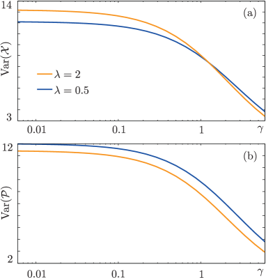
Figure 8: (Color online) Variance of the position $\mathcal{X}$ (a) and of the momentum $\mathcal{P}$ (b) as a function of $\gamma$. In all panels $\tau=9$, $eV=20\,\omega_{0}$, $n_{\mathrm{g}}=1/2$ and $\omega_{c}=10^{6}\ \omega_{0}$.

As expected, in the coherent regime both variances are strongly suppressed with respect to the large values attained in the diabatic regime, both for high and low (not shown) voltages. This fact denotes a tendency towards squeezing. mandel

III.5 Vibronic Fluctuations

The out-of-equilibrium vibron behavior is conveniently discussed introducing the vibron Fano factor merlo ; rod

$$F_{\rm{v}}=\frac{\mathrm{Var}(N)}{\langle N\rangle}\,,$$ (35)

where $N\equiv b^{{\dagger}}b$. Here, $F_{\rm{v}}$ is the ratio between the variance of the vibron occupation number $\mathrm{Var}(N)=\langle N^{2}\rangle-\langle N\rangle^{2}$ and its average $\langle N\rangle$, where $\langle\mathcal{O}\rangle=\mathrm{Tr}\{\mathcal{O}\rho\}=\mathrm{Tr}\{\mathcal{U}\mathcal{O}\mathcal{U}^{\dagger}\bar{\rho}\}$. This quantity (not be confused with the electronic Fano factor) brings information about the statistics of the vibronic mode and also on electronic properties, like charge fluctuations. This is due to the involved polaron transformation and it can be explicitly seen introducing the hybrid average $\langle\mathcal{O}\rangle_{\bar{\rho}}=\rm{Tr}\{\mathcal{O}\bar{\rho}\}$. In terms of $\langle\cdot\rangle_{\bar{\rho}}$ one has

$$\begin{split}\langle N\rangle=&\,\langle N\rangle_{\bar{\rho}}-\sqrt{2}\langle\hat{\eta}\mathcal{X}\rangle+\langle\hat{\eta}^{2}\rangle\\ \mathrm{Var}(N)=&\,\mathcal{V}(N)+\mathcal{V}(\hat{\eta}^{2})+2\mathcal{V}(\hat{\eta}\mathcal{X})+2\mathcal{C}(\hat{\eta}^{2},N)\\ &-\sqrt{2}\left[\mathcal{C}(\hat{\eta}\mathcal{X},N)+\mathcal{C}(N,\hat{\eta}\mathcal{X})+2\mathcal{C}(\hat{\eta}^{2},\hat{\eta}\mathcal{X})\right]\,,\end{split}$$ (36)

where $\mathcal{V}(\mathcal{O})\equiv\langle\mathcal{O}^{2}\rangle_{\bar{\rho}}-\langle\mathcal{O}\rangle^{2}_{\bar{\rho}}$ and $\mathcal{C}(\mathcal{A},\mathcal{B})\equiv\langle\mathcal{A}\mathcal{B}\rangle_{\bar{\rho}}-\langle\mathcal{A}\rangle_{\bar{\rho}}\langle\mathcal{B}\rangle_{\bar{\rho}}$, with adimensional oscillator position $\mathcal{X}$. The quantities $\langle N\rangle$ and $\mathrm{Var}(N)$ depend explicitly both on the charge (being $\hat{\eta}=\lambda(\hat{n}-n_{\rm{g}})$) and on its fluctuations. In Eq. (36) all terms of the form $\langle\cdot\,\mathcal{X}\rangle$ and $\mathcal{C}(\cdot,\,\cdot\,\mathcal{X})$ depend on the coherences of the density matrix. In the RWA these terms simplify but keep the $\hat{\eta}$ dependence. We remark that, beside the explicit dependence of $\mathrm{Var}(N)$ and $\langle N\rangle$ on $\langle n\rangle$, fluctuations of the electronic charge intrinsically affect $F_{\rm{v}}$, since the contribution of electronic and vibronic degrees of freedom cannot be factorized in $\bar{\rho}_{qq^{\prime}}^{n}$.
$F_{\rm{v}}$ belongs to the class of “bosonic” Fano factors, originally introduced to characterize boson distributions and often used to study photon populations in the context of quantum optics. mandel Typically, for bosons the Fano factor is super-Poissonian ($F_{\rm{v}}>1$). This is, for example, the situation for light from a classical radiation field. mandel Deviations from the super-Poissonian regime signal non-classical correlations, which have been observed for instance in experiments with micromaser. maser From an experimental point of view, the situation for vibron is more complicated than in the case of photons, although many proposals have been made to observe quantities like the average vibron number. santa ; buks ; woolley Recent experiments aiming at characterizing the vibron distributions have appeared. o_connel A few recent theoretical works investigated the vibron distributions predicting sub-Poissonian vibron Fano factor in the diabatic regime $\gamma\ll 1$, for low temperatures $\tau\ll 1$ and in selected parameter ranges. merlo ; cava3

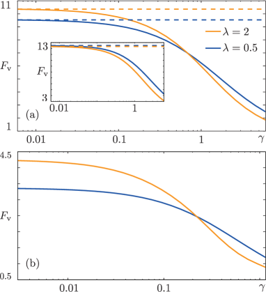
Figure 9: (Color online) Vibron Fano factor $F_{\rm{v}}$ as a function of $\gamma$ for different values of the electron-vibron coupling strength $\lambda$ and temperature $\tau$. In panel (a) $\tau=9$ and $eV=\omega_{0}$, in the inset $eV=20\ \omega_{0}$. In panel (b) $\tau=3$ and $eV=\omega_{0}$. Solid lines are the results obtained with the GME, dashed lines are obtained within the RWA. In all panels, $n_{\rm{g}}=1/2$ and $\omega_{\rm{c}}=10^{6}\ \omega_{0}$.

The behavior of the vibron Fano factor as a function of $\gamma$ for weak and strong $\lambda$ is reported in Fig. 9. In the regimes where the vibron can be approximated by an effective thermal distribution, $F_{\rm{v}}$ displays a super-Poissonian behavior. This occurs in the diabatic regime, both at low and high voltages ($eV$ smaller or larger than $k_{\rm{B}}T$), and in the weakly coherent regime. In this case however the vibron Fano factor is considerably reduced. These behaviors qualitatively do not depend on the electron-vibron coupling $\lambda$. In the diabatic regime the RWA applies with no dependence on $\gamma$.
On the other hand, entering the strongly coherent regime ($\gamma\approx 1$ and $\tau=3$ in Fig. 9(b)), non-classical sub-Poissonian vibron Fano factors are obtained. This is in correspondence with the negative values of the Wigner function observed in this parameter regime. Both features result from the large vibronic coherences. Similar conclusions were drawn from the frequency-dependent shot noise of a NEMS. brandes1 Here, however, these peculiar quantum behaviors show up in the steady state regime.

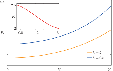
Figure 10: (Color online) Main: plot of $F_{\rm{v}}$ as a function of $V$ (units $\omega_{0}/e$) for different values of $\lambda$. Inset: dependence of $F_{\rm{v}}$ on the electron-vibron strength $\lambda$, for $eV=15\,\omega_{0}$. Other parameters are $\gamma=6$, $n_{\rm{g}}=1/2$, $\tau=9$ and $\omega_{\rm{c}}=10^{6}\ \omega_{0}$.

The vibron Fano factor also depends on the voltage and on electron-vibron coupling. $F_{\rm{v}}$ increases with increasing bias voltage, assuming super-Poissonian values even in the coherent regime, Fig. 10 (main panel). This behavior can be attributed to the increase of scattering between oscillator states induced by the current flow across the system. In the inset, the Fano factor is plotted as a function of $\lambda$: $F_{\rm{v}}$ decreases with increasing coupling strengths. This trend has been found both in the low ($eV<k_{\rm B}T$) and in the high ($eV>k_{\rm B}T$) voltage regimes - see also Figs. 9(a) - (b).

III.6 Charge degree of freedom

We conclude the survey of our results briefly commenting on the electronic properties. Figure 11(a) shows the $I(V)$ characteristics for different values of $\gamma$. In the regime $\tau>1$, the vibron sideband can not be resolved and the current increases monotonically.

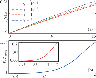
Figure 11: (Color online) (a) Current $I$ (units $e\Gamma_{0}$) as a function of $V$ (units $\omega_{0}/e$) for different values of $\gamma$. (b) Ratio between the current obtained with the GME ($I$) and the current in the RWA approximation ($I_{\rm{RWA}}$) as a function of $\gamma$, at $eV=15\,\omega_{0}$. Inset: average occupation $\langle n\rangle$ of the electronic level. Other parameters: $n_{\rm{g}}=1/2$, $\tau=9$, $\lambda=2$ and $\omega_{c}=10^{6}\ \omega_{0}$.

Figure 11(b) shows the ratio between the current $I$ obtained from the GME and the current in the RWA, $I_{\rm{RWA}}$, as a function of $\gamma$ and fixed voltage $V$. Increasing $\gamma$, the current increases with respect to the RWA limit. This qualitative trend occurs in all the parameter regimes explored. The increase of the current is more prominent for larger values of $\lambda$. This is a consequence of the delocalization of the vibron density matrix occurring with increasing electron-vibron coupling.
The average occupation of the electronic dot level $\langle\hat{n}\rangle$ behaves similarly to the current (Fig. 11 inset). For the case of only $n=0$ and $n=1$ electron states the variance of the electron occupation number reads

$$\mathrm{Var}(\hat{n})=\langle\hat{n}^{2}\rangle-\langle\hat{n}\rangle^{2}=\langle\hat{n}\rangle\left(1-\langle\hat{n}\rangle\right)\,.$$ (37)

The increase of $\langle\hat{n}\rangle>1/2$ signals a suppression of the fluctuations of the electronic level population analogously to the fluctuations of the vibronic part.

IV conclusions

In the present article we derived a generalized master equation to explore the steady-state properties of a nano-electromechanical system in a wide parameters range. extends from the very fast vibrations $\omega_{0}\gg\Gamma_{0}$ to the slow, coherent regime where the off-diagonal elements of the reduced density matrix between energy eigenstates are paramount.
In the coherent regime, two peculiar behaviors have been found. For intermediate frequencies, $\omega_{0}\approx\Gamma_{0}$, the system can be described in terms of an effective thermal distribution with a temperature lower than that of the environment. The cooling phenomenon is accompanied by a decrease of position and momentum quadratures. For still slower oscillations, a strongly coherent regime is entered characterized by non classical behavior. A benchmark of this regime is a marked suppression of the vibron Fano factor, which can even attain sub-Poissonian values.
This work is one of the first steps towards the understanding of dynamical properties of nano-electromechanical systems in the coherent regime and represents a rather tough numerical challenge, due to the slow convergence of the master equation solution and the need of a large number of basis states. Future investigations are certainly in order, to explore the regime of very strong electron-vibron coupling and the crossover towards the semi-classical regime. Further interesting issues to be investigated are higher order electronic properties, like the current fluctuations and their connection with the fluctuations of the mechanical part.

Acknowledgments. The authors acknowledge stimulating discussions with A. Nocera. Financial support by CNR-SPIN via both the Seed Project PLASE001 and the “Progetto giovani”, and by the EU-FP7 via ITN-2008-234970 NANOCTM is also gratefully acknowledged.

References

- (1) M. L. Roukes, Nanoelectromechanical Systems, in Technical Digest of the 2000 Solid State Sensor and Actuator Workshop, Transducers Research Foundation, Cleveland, OH (2000).
- (2) H. Park, J. Park, A. K. L. Lim, E. H. Anderson, A. P. Allvisatos, and P. McEuen, Nature 407, 57 (2000).
- (3) R. Leturcq, C. Stampfer, K. Inderbitzin, L. Durrer, C. Hierold, E. Mariani, M. G. Schultz, F. von Oppen, and K. Ensslin, Nature Phys. 5, 327 (2009).
- (4) B. J. Leroy, S. G. Lemay, J. Kong, and C. Dekker, Nature 432, 371 (2004).
- (5) S. Sapmaz, P. Jarillo-Herrero, Y. M. Blanter, C. Dekker, and H. S. J. van der Zant, Phys. Rev. Lett. 96, 026801 (2006).
- (6) B. Lassagne, Y. Tarakanov, J. Kiranet, D. Garcia-Sanchez, and A. Bachtold, Science 325, 1107 (2009).
- (7) R. G. Knobel and A. N. Cleland, Nature 424, 291 (2003).
- (8) E. M. Weig, R. H. Blick, T. Brandes, J. Kirschbaum, W. Wegscheider, M. Bichler, and J. P. Kotthaus, Phys. Rev. Lett. 92, 046804 (2004).
- (9) J. Koch, F. von Oppen, and A. V. Andreev, Phys. Rev. B 74, 205438 (2006).
- (10) A. Mitra, I. Aleiner, and A. J. Millis, Phys. Rev B 69, 245302 (2004).
- (11) S. Braig and K. Flensberg, Phys. Rev. B 68, 205324 (2003).
- (12) X. Y. Shen, B. Dong, X. L. Lei, and N. J. M. Horing, Phys. Rev. B 76, 115308 (2007).
- (13) A. Zazunov, D. Feinberg, and T. Martin, Phys. Rev. B 73, 115405 (2006).
- (14) F. Cavaliere, A. Braggio, J. T. Stockburger, M. Sassetti, and B. Kramer, Phys. Rev. Lett. 93, 036803 (2004).
- (15) A. Braggio, M. Sassetti, and B. Kramer, Phys. Rev. Lett. 87, 146802 (2001).
- (16) F. Cavaliere, A. Braggio, M. Sassetti, and B. Kramer, Phys. Rev. B 70, 125323 (2004).
- (17) F. Haupt, F. Cavaliere, R. Fazio, and M. Sassetti Phys. Rev. B 74, 205328 (2006).
- (18) J. A. Sidles, J. L. Garbini, K. J. Bruland, D. Rugar, O. Züger, S. Hoen, and C. S. Yannoni, Rev. Mod. Phys. 67, 249 (1995).
- (19) B. Ilic, H. G. Craighead, S. Krylov, W. Senaratne, C. Ober, and P. Neuzil, J. Appl. Phys. 95, 3694 (2004).
- (20) A. K. Naik, M. S. Hanay, W. K. Hiebert, X. L. Feng, and M. L. Roukes, Nature Nanotech. 4, 445 (2009).
- (21) F. Giazotto, T. Heikkilä, A. Luukanen, A. M. Savin, and J. P. Pekola, Rev. Mod. Phys. 78, 217 (2006).
- (22) L. Mandel and E. Wolf, Optical Coherence and Quantum Optics, N. Y. : Cambridge University Press, 1995.
- (23) J. B. Hertzberg, T. Rocheleau, T. Ndukum, M. Savva, A. A. Clerk, and K. C. Schwab, Nature Phys. 6, 213 (2010).
- (24) J. Koch and F. von Oppen, Phys. Rev. Lett. 94, 206804 (2005).
- (25) D. Mozyrsky, M. B. Hastings, and I. Martin, Phys. Rev. B 73, 035104 (2006).
- (26) A. Nocera, C. A. Perroni, V. Marigliano Ramaglia, and V. Cataudella, Phys. Rev. B 83, 115420 (2011).
- (27) R. Hussein, A. Metelmann, P. Zedler, and T. Brandes, Phys. Rev. B 82, 165406 (2010).
- (28) M. Merlo, F. Haupt, F. Cavaliere, and M. Sassetti, New. J. Phys. 10, 023008 (2008).
- (29) F. Cavaliere, G. Piovano, E. Paladino, and M. Sassetti, New J. Phys 10, 115004 (2008).
- (30) A. D. Armour, M. P. Blencowe, and Y. Zhang, Phys. Rev. B 69, 125313 (2004).
- (31) A. D. Armour, Phys. Rev. B 70, 165315 (2004).
- (32) C. B. Doiron, W. Belzig, and C. Bruder, Phys. Rev. B 74, 205336 (2006).
- (33) T. J. Harvey, D. A. Rodrigues, and A. D. Armour, Phys. Rev. B 81, 104514 (2010).
- (34) T. J. Harvey, D. A. Rodrigues, and A. D. Armour, Phys. Rev. B 78, 024513 (2008).
- (35) D. A. Rodrigues, J. imbers, T. J. Harvey, and A. D. Armour, New J. Phys. 9, 84 (2007).
- (36) A. A. Clerk and S. Bennett, New J. Phys. 7, 238 (2005).
- (37) L. P. Kouwenhoven, C. M. Marcus, P. L. McEuen, S. Tarucha, R. M. Westervelt, N. S. Wingreen Electron transport in quantum dots, edited by L. L. Sohn, L. P. Kouwenhoven, and G. Schön, Kluwer Series E345, 1997.
- (38) S. H. Ouyang, J. Q. You, and F. Nori, Phys. Rev. B 79, 075304 (2009).
- (39) D. A. Rodrigues and A. D. Armour, New J. Phys. 7, 251 (2005).
- (40) F. Pistolesi, J. of Low Temp. Phys. 154, 199 (2009).
- (41) F. Pistolesi, Ya. M. Blanter, and I. Martin, Phys. Rev. B 78, 085127 (2008).
- (42) M. G. Schultz, Phys. Rev. B 82, 195322 (2010).
- (43) W. Izumida and M. Grifoni, New J. Phys. 7, 244 (2005).
- (44) K. Flensberg, New J. Phys 8, 5 (2006).
- (45) F. Cavaliere, E. Mariani, R. Leturcq, C. Stampfer, and M. Sassetti, Phys. Rev. B 81, 201303(R) (2010).
- (46) M. Galperin, A. Nitzan, and M. A. Ratner, Phys. Rev. B 73 045314 (2006).
- (47) M. Galperin, M. A. Ratner, and A. Nitzan, Nano Lett. 5 125 (2005).
- (48) I. Wilson-Rae, N. Nooshi, W. Zwerger, and T. J. Kippenberg, Phys. Rev. Lett. 99, 093901 (2007).
- (49) J. D. Teufel, J. W. Harlow, C. A. Regal, and K. W. Lehnert, Phys. Rev. Lett. 101, 197203 (2008).
- (50) J. D. Teufel, T. Donner, M. A. Castellanos-Beltran, J. W. Harlow, and K. W. Lehnert, Nature Nanotech. 4, 820 (2009).
- (51) P. Rabl, Phys. Rev. B 82, 165320 (2010).
- (52) S. Zippilli, A. Bachtold, and G. Morigi, Phys. Rev. B 81, 205408 (2010).
- (53) R. Ruskov, K. Schwab, and A. N. Korotkov, Phys. Rev. B 71, 235407 (2005).
- (54) A. A. Clerk, F. Marquardt, and K. Jacobs, New J. Phys. 10, 095010 (2008).
- (55) R. El Boubsi, O. Usmani, and Y. M. Blanter, New J. Phys. 10, 095011 (2008).
- (56) R. Sanchez, G. Platero, and T. Brandes, Phys. Rev. Lett 98, 146805 (2007).
- (57) R. Sanchez, G. Platero, and T. Brandes, Phys. Rev. B 78, 125308 (2008).
- (58) O. Usmani, Y. M. Blanter, and Y. V. Nazarov, Phys. Rev. B 75, 195312 (2007).
- (59) D. Mozyrsky, I. Martin, and M. B. Hastings, Phys. Rev. Lett. 92, 018303 (2004).
- (60) M. Galperin, A. Nitzan, and M. A. Ratner, J. Phys.: Condens. Matter 20, 374107 (2008).
- (61) K. Blum, Density Matrix Theory and Application, Plenum Press, New York (1996).
- (62) H. Huebener and T. Brandes, Phys. Rev. Lett. 99, 247206 (2007).
- (63) D.A. Rodrigues, J. Imbers, and A. D. Armour, Phys. Rev. Lett. 98, 067204 (2007).
- (64) T. Novotný, A. Donarini, C. Flindt, and A.-P. Jauho, Phys. Rev. Lett. 92, 248302 (2004).
- (65) T. Novotný, A. Donarini, and A.-P. Jauho, Phys. Rev. Lett. 90, 256801 (2003).
- (66) M. G. Schultz, Phys. Rev. B 82, 155408 (2010).
- (67) J. Konig, J. Schmid, H. Schoeller, and G. Schon, Phys. Rev. B 54, 16820 (1996).
- (68) C. Timm, Phys. Rev. B 77, 195416 (2008).
- (69) S.A. Gurvitz and Y.S. Prager, Phys. Rev. B 53, 15932 (1996).
- (70) M. Abramovitz, I. Stegun, Handbook of Mathematical Functions with Formulas, Graphs, and Mathematical Tables, Dover, 1964.
- (71) H. Schoeller and J. König, Phys. Rev. Lett. 84, 3686 (2000).
- (72) G. Rempe, F. Schmidt-Kaler, and H. Walther, Phys. Rev. Lett. 64, 2783 (1990).
- (73) D. H. Santamore, A. C. Doherty, and M. C. Cross, Phys. Rev. B 70, 144301 (2004).
- (74) E. Buks, E. Segev, S. Zaitsev, B. Abdo, and M. P. Blencowe, Eur. Phys. Lett. 81, 10001 (2008).
- (75) M. J. Woolley, A. C. Doherty, and G. J. Milburn, Phys. Rev. B 82, 094511 (2010).
- (76) A. D. O’Connell, M. Hofheinz, M. Ansmann, R. C. Bialczak, M. Lenander, Erik Lucero, M. Neeley, D. Sank, H. Wang, M. Weides, J. Wenner, John M. Martinis, and A. N. Cleland, Nature 464, 697 (2010).