Problems of astrophysical turbulent convection:
thermal convection in a layer without boundaries

Thermal convection in fluid layers heated from below are usually realized experimentally as well as treated theoretically with fixed boundaries on which conditions for the temperature and the velocity field are prescribed. The thermal and velocity boundary layers attached to the upper and lower boundaries determine to a large extent the properties of turbulent convection at high Rayleigh numbers. Fixed boundaries are often absent in natural realizations of thermal convection. This paper studies the properties of convection driven by a planar heat source below a cooling source of equal size immersed in an otherwise stably stratified fluid layer are studied in this paper. Unavoidable boundaries do not influence the convection flow since they are separated from the active convection layer by nearly motionless stably stratified regions. The onset of convection occurs in an inner unstably stratified region where the mean temperature gradient is reversed. But the region of a reversed horizontally averaged temperature gradient disappears at higher amplitudes of convection such that the vertical derivative of the mean temperature no longer changes its sign.  

1 Introduction

High Rayleigh number thermal convection has received much attention in the past decades for several reasons. On the one hand, thermal convection represents the most common fluid flow in nature and the understanding of its properties is essential for assessing energy transports in planetary atmospheres and in stars. On the other hand, turbulent convection has become the paradigmatic example for the study of turbulent transports. The experimental investigations are facilitated by the fact that unlike the situation in channel flows, the advection of turbulent eddies by a mean flow is absent. Moreover, the temperature as a scalar quantity offers additional opportunities for quantitative observations. These properties have also motivated theoretical studies, and numerous computational simulations have appeared in the recent literature. For an overview of many aspects of convection we refer to the recent book by [Lappa (2010)].

A common property of laboratory convection experiments as well as of theoretical formulations of convection problems is the assumption of fixed boundaries on which the temperature is prescribed and the velocity field usually must vanish. As a result, turbulent convection is determined to a large extent by the properties of the thermal and velocity boundary layers forming at the fixed upper and lower boundaries. This situation is not typical for most convection flows realized in nature. Often convection is driven by heat sources owing to absorbed radiation in conjunction with cooling by emitted radiation. An example for such a convection system is the solar convection zone in which heat is partly transported by convection in the region where a purely radiative transport would require an unstable superadiabatic gradient of entropy.

In this paper we are not interested in studying any realistic convection layer. Instead, we are formulating a theoretical problem in which convection without influence from boundaries can be investigated in a simple setting. We have chosen the case of a heat source layer below a cooling layer of equal size. Both are embedded in a extended, stably stratified fluid layer such that the velocity field is strongly damped above and below the heating and cooling layers. The unavoidable boundaries introduced for the numerical analysis thus exert only a minimal influence on the convection flow.

In the following section the mathematical problem is described. Numerical simulation of two-dimensional convection for different Prandtl numbers is carried out and the results are discussed in Section 3. An outlook on future work is given in Section 4.

2 Mathematical formulation of the problem

We consider a fluid layer of height $h$ and adopt the Boussinesq approximation, i.e., all material properties are assumed to be constant except for the temperature dependence of the density which is taken into account only in connection with the gravity term. Using as scales the length $h$, the time $h^{2}/\kappa$, where $\kappa$ is the thermal diffusivity of the fluid, and the temperature $qh^{2}/c\kappa$, where $q$ is a heat source density and $c$ is the specific heat of the fluid, we obtain the dimensionless equations of motion for the velocity vector $\vec{u}$ and the heat equation for the deviation $\Theta$ from the static temperature distribution, $T_{s}$

$$\begin{aligned} (\partial_{t}\vec{u}+\vec{u}\cdot\nabla\vec{u})/P&=-\nabla\pi+R\Theta\vec{k}+\nabla^{2}\vec{u},\\ \nabla\cdot\vec{u}&=0,\\ \partial_{t}\Theta+\vec{u}\cdot\nabla\Theta&=u_{z}T^{\prime}_{s}+\nabla^{2}\Theta,\end{aligned}$$ (1a)

where $\partial_{t}$ denotes the partial derivative with respect to time $t$ and where all terms in the equation of motion that can be written as gradients have been combined into $\nabla\pi$. The dimensionless parameter, the Rayleigh number $R$ and the Prandtl number $P$ are given by

$$R=\frac{\alpha gqd^{6}}{c\nu\kappa},\qquad P=\frac{\nu}{\kappa},$$ (2)

where $\alpha$ is the coefficient of thermal expansion, $g$ is gravity and $\nu$ is the kinematic viscosity. We shall use a cartesian system of coordinates with the $z$-coordinate and the unit vector $\vec{k}$ in the direction opposite to gravity. A heat source distribution antisymmetric with respect to $z=0$ is chosen such that the static temperature distribution, $T_{s}(z)$, is governed by the equation

$$\frac{d^{2}T_{s}}{dz^{2}}=\frac{2\gamma\tanh\gamma z}{(\cosh\gamma z)^{2}},$$ (3)

where $\gamma$ is assumed to be large in comparison to unity such that heat and cooling sources are finite only close to $z=0$ and decay rapidly towards the boundaries at $z=\pm 1/2$. Integration of Eq. (2.3) yields

$$\frac{dT_{s}}{dz}=\beta-\frac{1}{(\cosh\gamma z)^{2}}\quad\text{and}\quad T_{s}(z)=\beta z-\frac{1}{\gamma}\tanh\gamma z,$$ (4)

where $\beta$ measures the stable stratification. We shall use stress-free boundary conditions and require that the $z$-derivative of $\Theta$ also vanishes,

$$u_{z}=\partial^{2}_{zz}u_{z}=\partial_{z}\Theta=0 \enspace\mbox{ at }\enspace z=\pm\frac{1}{2}.$$ (5)

In solving the problem described by Eqs. (2.1) and (2.5) we start with the two-dimensional case in which the velocity field can be described by a stream function,

$$u_{z}=\frac{\partial\phi}{\partial x},\qquad u_{x}=-\frac{\partial\phi}{\partial z}.$$ (6)

The equations for the stream function $\phi$, the vorticity $V$ and deviation $\Theta$ of the temperature from its static distribution can now be written in the form

$$V=-\nabla^{2}\phi,$$ (7a)

$$(\partial_{t}V-\partial_{z}\phi\partial_{x}V+\partial_{x}\phi\partial_{z}V)/P-\nabla^{2}V=-R\partial_{x}\Theta,$$ (7b)

$$\partial_{t}\Theta-\partial_{z}\phi\partial_{x}\Theta+\partial_{x}\phi\partial_{z}\Theta=-\partial_{x}\phi T^{\prime}_{s}+\nabla^{2}\Theta,$$ (7c)

which can be solved more easily than the original equations since the pressure gradient has been eliminated. In the horizontal $x$-direction periodic boundary conditions will be applied at $x=\pm\Gamma/2$. The boundary conditions (Eq. 2.5) now assume the form

$$\phi=V=\partial_{z}\Theta=0 \enspace\mbox{ at }\enspace z=\pm\frac{1}{2}.$$ (8)

In the following analysis we shall restrict attention to the case $\beta=0.5$ and $\gamma=10$ which is representative for a narrow convection layer imbedded in a wider stably stratified layer.

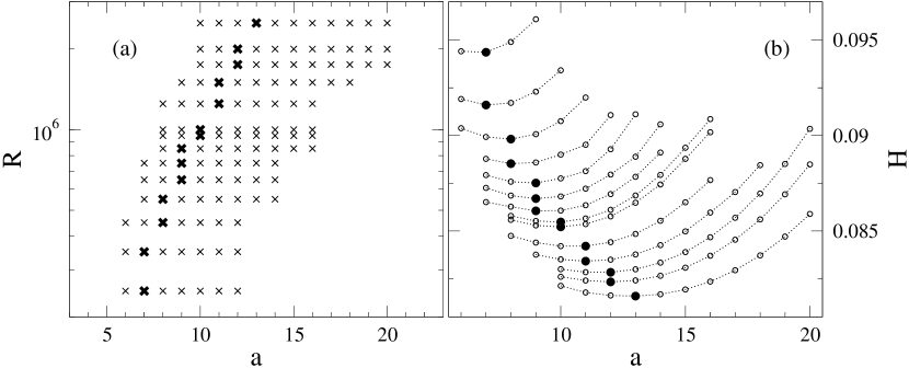
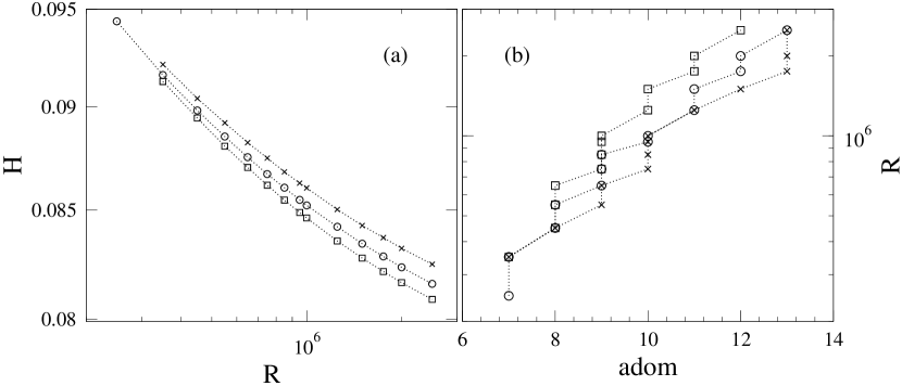
Figure 1: Range of wavenumbers of convection rolls for $P=1$, $\gamma=10$, $\beta=0.5$. (a) The range of possible roll wavenumbers $a$ for a given Rayleigh number $R$, with the dominant one indicated by a thick cross. (b) The value of $H\equiv\beta/2-T(1/2)$ as a function of the values of possible roll wavenumbers $a$. The dominant wavenumber is that which minimizes $H$. The values of $R$ in (b) are the same as those in (a).

Figure 2: (a) The quantity $H\equiv\beta/2-T(1/2)$ at the upper boundary, and (b) the dominant wavenumber versus the Rayleigh number $R$ for $P=0.5$ (crosses), $P=1$ (circles), $P=10$ (squares) in the case $\gamma=10$, $\beta=0.5$.

For the numerical solution of Eqs. (2.7) and (2.8) we have adopted the finite-element method as implemented in the commercially-available software platform COMSOL v. 3.5 [COMSOL] For the spatial discretization we have used regular rectangular meshes typically consisting of 19200 elements and Lagrange shape functions. For the time integration we have used a backward-difference formula of order 4 with adaptive step control. The relative and the absolute error tolerances have been set to $10^{-6}$ and $10^{-8}$, respectively.

3 Two-dimensional convection

The critical Rayleigh number $R_{c}$ for onset of convection and the corresponding wavenumber $a_{c}$ in the case $\beta=0.5$ and $\gamma=10$ can be determined numerically with a shooting method. The result

$$R_{c}=144095,\qquad a_{c}=5.86$$ (9)

indicates that for $R>R_{c}$ convection rolls with the wavelength $2\pi/\alpha_{c}$ grow and become asymptotically steady solutions as verified by the nonlinear analysis described below. The relatively high values (Eq. 3.1) – as compared with the values $R_{c}=6.75\pi^{4}$ with $\alpha_{c}=\pi/\sqrt{2}$ for the corresponding Rayleigh-Bénard problem – reflect the reduction of the height of the convecting region from the total height of the layer. The result is not sensitive to the applied boundary conditions (Eq. 2.8). When the thermal boundary condition is replaced by $\Theta=0$ at $z=\pm\frac{1}{2}$, the result

$$R_{c}=145154,\qquad a_{c}=5.90$$ (10)

is obtained.

As the Rayleigh number increases beyond the critical value, the preferred wavenumber of finite amplitude convection increases as the wavelength of convection assumes values corresponding to the typical thickness of the order of $1/\gamma$ of the most strongly convecting part of the layer. As indicated in Fig. 1(a), there is a finite spread of wavenumbers that can be realized at supercritical Rayleigh numbers. Here, all integer values have been indicated for which computations with $\Gamma=2\pi/a$ gave solutions with just a single wavelength of convection, i.e., with two counter-rotating rolls. Beyond the highest value of the wavenumber $a$ at a given value of the Rayleigh number $R$, no finite-amplitude solution could be obtained. It appears that at a given value of $R$ the convection pattern that is realized from random initial conditions in the case of a large $\Gamma$, say $\Gamma=10$, is close to that which maximizes $\overline{\Theta}(z=0.5)$ where the bar indicates the $x$-average. For this reason, the quantity $H\equiv\beta/2-T(0.5)=-\overline{\Theta}(0.5)+(\tanh\gamma z)/\gamma$ has been plotted in Fig. 1(b) for the same solutions as indicated in Fig. 1(a). At the preferred value of the wavenumber $a$, the quantity $H$ assumes a minimum which is approximately indicated by the closest integer value of $a$.

In Fig. 2(a) the quantity $H$ has been plotted as a function of $R$ for different values of the Prandtl number $P$. Computations at much higher values of $R$ appear to indicate that $H$ tends to zero for $R\rightarrow\infty$. But these values of $R$ have not been included in Fig. 2 because of insufficient numerical accuracy. Corresponding values of $a$ are displayed in Fig. 2(b) which indicates that the preferred $a$ does not vary much with the Prandtl number $P$.

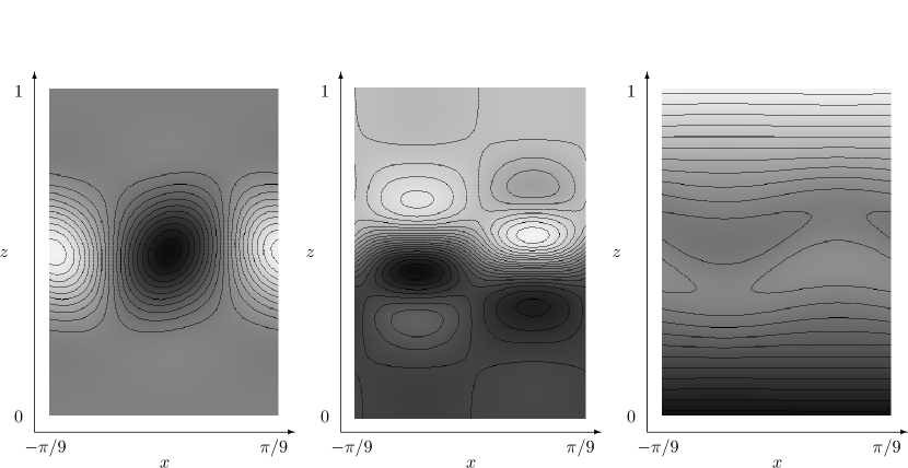
Figure 3: Patterns of convection in the case $P=1$, $R=850000$, $\gamma=10$, $\beta=0.5$, corresponding to a single wavelength of the dominant wavenumber $a=9$. The first, second and third plots show $\phi$, $\Theta$ and $T=T_{s}+\Theta$, respectively. Whiter shades correspond to negative values and darker shades to positive values.

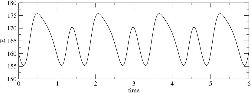
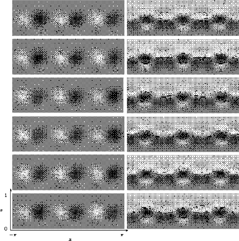
Figure 4: Time series of the kinetic energy in the case $P=0.1$, $R=850000$, $\gamma=10$, and $\beta=0.5$.

Figure 5: A period of oscillations in the case shown in Fig. 4. The left and the right columns shows contour plots of $\phi$ and $\Theta$, respectively. The time interval between two plots is $0.32$ such that approximately one period is covered.

Typical convection patterns corresponding to the dominant wavenumber of convection are shown in Fig. 3. These patterns are stationary due to the restriction of the horizontal size of the domain to $\Gamma=2\pi/a$, which forces the system to select a single wavenumber. As the aspect ratio of the domain is increased, temporal and spatial modulation of the patterns occur especially for large values of the Rayleigh number $R$ and for smaller values of the Prandtl number $P$. As an example, Figs. 4 and 5 illustrate a time-dependent modulation with the wavelength of $\Gamma$, which in this case is set to $\Gamma=6\pi/a$.

A most surprising phenomenon is exhibited in Fig. 6 where the mean temperature, $T_{s}(z)+\overline{\Theta}$, and the mean temperature gradient have been plotted in 6(a) and 6(b), respectively. Unexpectedly, the region of decreasing mean temperature with height characterizing the onset of convection gives way to a purely increasing mean temperature with height as the Rayleigh number exceeds about twice its critical value. This effect is even more visible if the quantity $G\equiv\tanh(\gamma z)/\gamma-\overline{\Theta}$ is plotted as a function of the vertical coordinate $z$ as shown in Fig. 7. Although a stably stratified layer is thus achieved in the mean, convection flows continue to be vigorous since they are driven by self-created horizontal temperature differences. The results do not depend much on the value of the Prandtl number.

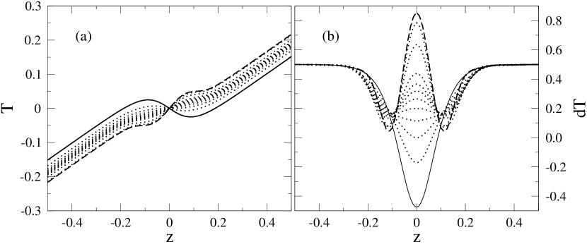
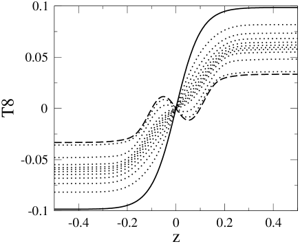
Figure 6: (a) $T=T_{s}+\overline{\Theta}$ and (b) $\partial_{z}T=\partial_{z}(T_{s}+\overline{\Theta})$ as a function of the vertical coordinate $z$ for $P=10$, $\gamma=10$, $\beta=0.5$ and $R=150000+i\times 10^{5}$, $i=0..7$, $R=$1050000, 2000000, 4000000, 6000000. The solid line indicates $R=150000$, the broken line indicates $R=6000000$ and the dotted lines indicate the intermediate values of $R$.

Figure 7: The quantity $G\equiv\tanh(\gamma z)/\gamma-\overline{\Theta}$ as a function of the vertical coordinate $z$ with the same parameter values and linetypes as in Fig. 6.

4 Discussion and outlook

Our study has been restricted in several aspects. We have focused on an idealized case with antisymmetric heating (cooling) and have not varied the parameters $\gamma$ and $\beta$. No comparison with naturally occurring systems has been attempted. Most importantly, we have considered in this report only a two-dimensional formulation. Further within this setting, we have performed the main part of our simulations so as to confine the flow to one of the possible roll wavenumbers. This has been done in order to investigate the behavior of the system in its simplest manifestation. We have found the unexpected effect that convection is driven by lateral variations in temperature even at moderate values of the Rayleigh number. We expect that this will result in patterns and dynamics quite different from those familiar from the case of the Rayleigh-Bénard problem in horizontal layers without stably stratified regions. In particular, we expect to find complex time-dependent behavior, a possibility clearly indicated by results such as the case presented in Figs. 4 and 5, as well as by our preliminary three-dimensional simulations, an example of which is shown in Fig. 8. Thus, a main goal in the 3D-case will be to study time dependences and the possibility of interaction with internal waves in the stably stratified regions of the layer.

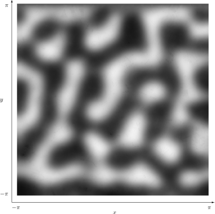
Figure 8: Three-dimensional patterns of convection in the case $P\to\infty$, $R=10^{6}$, $\beta=0.5$, $\gamma=10$ visualized by a grey-scale map of $\theta$ in the plane $z=0$.

Acknowledgments We gratefully acknowledge the support of CTR and NASA which made possible our visits to Stanford. The COMSOL software has been licensed to the School of Mathematics and Statistics of the University of Glasgow, UK.

References

- [COMSOL] COMSOL Group, The 2010 COMSOL version 3.5, www.comsol.com.
- [Lappa (2010)] Lappa, M. 2010 Thermal Convection: Patterns, Evolution and Stability. John Wiley & Sons, Hoboken, NJ.