Turbulent three-dimensional MHD dynamo model in spherical shells: Regular oscillations of the dipolar field

We report the results of three-dimensional numerical simulations of convection-driven dynamos in relatively thin rotating spherical shells that show a transition from an strong non-oscillatory dipolar magnetic field to a weaker regularly oscillating dipolar field. The transition is induced primarily by the effects a stress-free boundary condition. The variation of the inner to outer radius ratio is found to have a less important effect.

 

1 Introduction

The Sun possesses a deep layer of intensely turbulent convection near its surface. The dynamical properties of this zone continue to elude basic physical explanation. The most important questions involve the solar differential rotation profile and the periodicity of the solar magnetic activity. The differential rotation is known from helioseismological studies (e.g. [Schou et al., 1998]): the angular velocity variation observed at the surface where the rotation is faster near the equator and slower near the poles, extends through the convection zone with little radial dependence. The basic feature of the solar activity is the existence of a periodic 22-year long cycle which is mainly manifested in the periodic appearance of sunspots accompanied by an oscillation of the antisymmetric (dipolar) parts of the solar magnetic field during which it reverses polarity (e.g. [Brandenburg & Subramanian, 2005]). Both the differential rotation and the solar activity cycle are persistent global scale features of the Sun and it is difficult to understand how they emerge from the intensely turbulent flow in the solar convection zone which includes scales ranging from granules (1 Mm in horizontal size), to supergranules (30 Mm), and possibly giant cells (over 200 Mm) and which shows similar contrasts in time scales. A variety of modeling approaches ranging from linear theory (e.g. [Rüdiger & Hollerbach, 2004]) and weakly nonlinear theory ([Busse, 1970]) to high-resolution three-dimensional global simulations of compressible convective dynamos in spherical shells ([Brun & Toomre, 2002], [Browning, 2007]) have been employed but the precise mechanisms leading to the peculiar form of the profile of solar differential rotation, and the regularity of its magnetic activity remain unclear.

In a recent study [Goudard & Dormy, 2008] carried out three-dimensional numerical simulations of self-excited convective dynamos with the aim of exploring the dependence of solutions on the thickness of the spherical shell. They employed a model that has been used as a benchmark by the geodynamo community ([Christensen et al., 2001]), which they modified by replacing the no-slip boundary conditions at the top of the spherical shell by stress-free ones. They found that a transition occurs from non-oscillating to regularly oscillating dipolar dynamo solutions as the thickness of the spherical shell is decreased and concluded that this is a purely geometric effect. They discussed their finding in the light of the facts that the outer core, the layer where the non-oscillatory geodynamo is believed to be generated is a relatively thick layer in the case of the Earth, whereas the solar convective zone is a relatively thin.

However, it is known that oscillating dipolar magnetic solutions can also be obtained in dynamos in thick spherical shells (Busse & Simitev 2006), and it remains unclear whether the transition found by Goudard & Dormy (2008) is the result of variation of the shell thickness or the introduction of a stress-free boundary condition. In this report we attempt to clarify this question and extend the results of Goudard & Dormy (2008) by exploring the effects of a different set of boundary conditions. We find that the transition to an oscillatory state is more likely due to the use of stress-free boundaries.

2 Mathematical formulation of the problem and methods of solution

We consider a spherical fluid shell rotating about a fixed vertical axis. We assume that a static state exists with the temperature distribution

$$T_{S}=T_{0}+\Delta T\eta r^{-1}(1-\eta)^{-2},$$

where $r$ denotes the distance from the center of the spherical shell, $\eta$ denotes the ratio of inner to outer radius of the shell and $d$ is its thickness, and $\Delta T$ is the temperature difference between the boundaries. The gravity field is given by

$$\mbox{\boldmath$g$}=-d\gamma\mbox{\boldmath$r$}.$$

In addition to $d$, the time $d^{2}/\nu$, the temperature $\nu^{2}/\gamma\alpha d^{4}$, and the magnetic flux density $\nu(\mu\varrho)^{1/2}/d$ are used as scales for the dimensionless description of the problem where $\nu$ denotes the kinematic viscosity of the fluid, $\kappa$ its thermal diffusivity, $\varrho$ its density and $\mu$ is its magnetic permeability. The equations of motion for the velocity vector $u$, the heat equation for the deviation $\Theta$ from the static temperature distribution, and the equation of induction for the magnetic flux density $B$ are thus given by

$$\partial_{t}\mbox{\boldmath$u$}+\mbox{\boldmath$u$}\cdot\nabla\mbox{\boldmath$u$}+\tau\mbox{\boldmath$k$}\times\mbox{\boldmath$u$}=-\nabla\pi+\Theta\mbox{\boldmath$r$}+\nabla^{2}\mbox{\boldmath$u$}+\mbox{\boldmath$B$}\cdot\nabla\mbox{\boldmath$B$},$$ (1a)

$$\nabla\cdot\mbox{\boldmath$u$}=0,$$ (1b)

$$\mathrm{P}(\partial_{t}\Theta+\mbox{\boldmath$u$}\cdot\nabla\Theta)=(\mathrm{R}\,\eta r^{-3}(1-\eta)^{-2})\mbox{\boldmath$r$}\cdot\mbox{\boldmath$u$}+\nabla^{2}\Theta,$$ (1c)

$$\nabla\cdot\mbox{\boldmath$B$}=0,$$ (1d)

$$\nabla^{2}\mbox{\boldmath$B$}=\mathrm{P}_{\mathrm{m}}(\partial_{t}\mbox{\boldmath$B$}+\mbox{\boldmath$u$}\cdot\nabla\mbox{\boldmath$B$}-\mbox{\boldmath$B$}\cdot\nabla\mbox{\boldmath$u$}),$$ (1e)

where $\partial_{t}$ denotes the partial derivative with respect to time $t$ and where all terms in the equation of motion that can be written as gradients have been combined into $\nabla\pi$. The Boussinesq approximation has been assumed in that the density $\varrho$ is regarded as constant except in the gravity term where its temperature dependence, given by $\alpha\equiv-({\rm\,d}\varrho/{\rm\,d}T)/\varrho=$const, is taken into account. The Rayleigh numbers $\mathrm{R}$, the Coriolis number $\tau$, the Prandtl number $\mathrm{P}$ and the magnetic Prandtl number $\mathrm{P}_{\mathrm{m}}$ are defined by

$$\mathrm{R}=\frac{\alpha\gamma\Delta Td^{4}}{\nu\kappa},\enspace\tau=\frac{2\Omega d^{2}}{\nu},\enspace\mathrm{P}=\frac{\nu}{\kappa},\enspace\mathrm{P}_{\mathrm{m}}=\frac{\nu}{\lambda},$$ (2)

where $\lambda$ is the magnetic diffusivity. Because the velocity field $u$ as well as the magnetic flux density $B$ are solenoidal vector fields, the general representation in terms of poloidal and toroidal components can be used

$$\mbox{\boldmath$u$}=\nabla\times(\nabla v\times\mbox{\boldmath$r$})+\nabla w\times\mbox{\boldmath$r$}\enspace,$$ (3a)

$$\mbox{\boldmath$B$}=\nabla\times(\nabla h\times\mbox{\boldmath$r$})+\nabla g\times\mbox{\boldmath$r$}\enspace.$$ (3b)

By multiplying the (curl)² and the curl of equation (1a) by $r$ we obtain two equations for $v$ and $w$

$$[(\nabla^{2}-\partial_{t}){\cal L}_{2}+\tau\partial_{\varphi}]\nabla^{2}v+\tau{\cal Q}w-{\cal L}_{2}\Theta=-\mbox{\boldmath$r$}\cdot\nabla\times[\nabla\times(\mbox{\boldmath$u$}\cdot\nabla\mbox{\boldmath$u$}-\mbox{\boldmath$B$}\cdot\nabla\mbox{\boldmath$B$})],$$ (4a)

$$[(\nabla^{2}-\partial_{t}){\cal L}_{2}+\tau\partial_{\varphi}]w-\tau{\cal Q}v=\mbox{\boldmath$r$}\cdot\nabla\times(\mbox{\boldmath$u$}\cdot\nabla\mbox{\boldmath$u$}-\mbox{\boldmath$B$}\cdot\nabla\mbox{\boldmath$B$}),$$ (4b)

where $\partial_{\varphi}$ denotes the partial derivative with respect to the angle $\varphi$ of a spherical system of coordinates $r,\theta,\varphi$ and where the operators ${\cal L}_{2}$ and $\cal Q$ are defined by

$${\cal L}_{2}\equiv-r^{2}\nabla^{2}+\partial_{r}(r^{2}\partial_{r}),$$

$${\cal Q}\equiv r\cos\theta\nabla^{2}-({\cal L}_{2}+r\partial_{r})(\cos\theta\partial_{r}-r^{-1}\sin\theta\partial_{\theta}).$$

The heat equation for the dimensionless deviation $\Theta$ from the static temperature distribution can be written in the form

$$\nabla^{2}\Theta+(\mathrm{R}\,\eta r^{-3}(1-\eta)^{-2}){\cal L}_{2}v=\mathrm{P}(\partial_{t}+\mbox{\boldmath$u$}\cdot\nabla)\Theta,$$ (5)

and the equations for $h$ and $g$ are obtained through the multiplication of equation (1e) and of its curl by $r$

$$\nabla^{2}{\cal L}_{2}h=\mathrm{P}_{\mathrm{m}}[\partial_{t}{\cal L}_{2}h-\mbox{\boldmath$r$}\cdot\nabla\times(\mbox{\boldmath$u$}\times\mbox{\boldmath$B$})],$$ (6a)

$$\nabla^{2}{\cal L}_{2}g=\mathrm{P}_{\mathrm{m}}[\partial_{t}{\cal L}_{2}g-\mbox{\boldmath$r$}\cdot\nabla\times(\nabla\times(\mbox{\boldmath$u$}\times\mbox{\boldmath$B$}))].$$ (6b)

In this report we discuss results obtained with two different sets of velocity boundary conditions, namely no-slip conditions given by

$$v=\partial_{r}v=w=0\qquad\mbox{ at }r=r_{i}\equiv\eta/(1-\eta)\mbox{ and }r=r_{o}\equiv 1/(1-\eta),$$ (7)

and mixed conditions, i.e. a combination of no-slip conditions at the inner spherical boundary and a stress-free condition at the outer boundary, given by

$$v=\partial_{r}v=w=0\qquad\mbox{ at }r=r_{i}\equiv\eta/(1-\eta),$$ (8)

$$v=\partial^{2}_{rr}v=\partial_{r}(w/r)=0\qquad\mbox{ at }r=r_{o}\equiv 1/(1-\eta).$$

As boundary conditions for the heat equation, we assume fixed temperatures

$$\Theta=0\qquad\mbox{ at }r=r_{i}\equiv\eta/(1-\eta)\mbox{ and }r=r_{o}\equiv 1/(1-\eta).$$ (9)

For the magnetic field, electrically insulating boundaries are assumed such that the poloidal function $h$ must be matched to the function $h^{(e)}$, which describes the potential fields outside the fluid shell

$$g=h-h^{(e)}=\partial_{r}(h-h^{(e)})=0\mbox{ at }r=r_{i}\equiv\eta/(1-\eta)\mbox{ and }r=r_{o}\equiv 1/(1-\eta).$$ (10)

But computations for the case of an inner boundary with no-slip conditions and an electrical conductivity equal to that of the fluid have also been done. The numerical integration of equations (4),(5), and (6) together with boundary conditions (9), (10) and any of (7) or (8), proceeds with the pseudo-spectral method as described by Tilgner (1999) which is based on an expansion of all dependent variables in spherical harmonics for the $\theta,\varphi$-dependences, i.e.

$$v=\sum\limits_{l,m}V_{l}^{m}(r,t)P_{l}^{m}(\cos\theta)\exp\{im\varphi\}$$ (11)

and analogous expressions for the other variables, $w,\Theta,h$ and $g$. Here $P_{l}^{m}$ denotes the associated Legendre functions. For the $r$-dependence expansions in Chebychev polynomials are used. For the computations to be reported in the following a minimum of 41 collocation points in the radial direction and spherical harmonics up to the order 128 have been used.

3 Dependence of convection and dynamo solutions on the thickness of the spherical shell

In order to clarify whether the transition from non-oscillatory to oscillatory dynamos reported by Goudard & Dormy (2008) is the exclusive result of variation in the radius ratio $\eta$, we started with a case similar to the one described in their work and identical to the geodynamo benchmark simulation described in (Christensen et al. 2001). More precisely, we employ no-slip boundary conditions, as given in the preceding section, both at the inner and outer surface of the shell. We then simulate a sequence of dynamo solutions where we increase the value of $\eta$ while keeping all other parameter values fixed.

Global quantities that characterize the basic properties of dynamo solutions include the magnetic energy density that can be decomposed into several components, namely poloidal and toroidal energy densities, each of which can be further decomposed into mean and fluctuating parts. The corresponding definitions are given by the expressions

$$\overline{M}_{p}=\frac{1}{2}\langle\mid\nabla\times(\nabla\overline{h}\times\mbox{\boldmath$r$})\mid^{2}\rangle,\quad\overline{M}_{t}=\frac{1}{2}\langle\mid\nabla\overline{g}\times\mbox{\boldmath$r$}\mid^{2}\rangle,$$

$$\widetilde{M}_{p}=\frac{1}{2}\langle\mid\nabla\times(\nabla\widetilde{h}\times\mbox{\boldmath$r$})\mid^{2}\rangle,\quad\widetilde{M}_{t}=\frac{1}{2}\langle\mid\nabla\widetilde{g}\times\mbox{\boldmath$r$}\mid^{2}\rangle,$$

where $\langle\cdot\rangle$ indicates the average over the fluid shell and $\overline{h}$ refers to the axisymmetric component of $h$. $\widetilde{h}$ is defined by $\widetilde{h}=h-\overline{h}$. Similarly, kinetic energy densities $\overline{E}_{p}$, $\overline{E}_{t}$, $\widetilde{E}_{p}$, and $\widetilde{E}_{t}$ can be defined with analogous expressions where $v$ and $w$ replace $h$ and $g$. In addition, the energy densities can be divided into those of fields that are antisymmetric (axial dipole symmetry) and those that are symmetric (axial quadrupole symmetry) with respect to the equatorial plane. The dipole (quadrupole) fields are described by spherical harmonic $Y_{l}^{m}$ with odd (even) $l+m$.

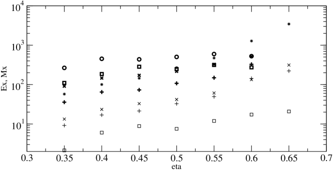
Figure 1: The averaged magnetic, $M$, and kinetic, $E$, energy density components, and the helicity, He, as a function of the radius ratio $\eta$ for fixed values of the other parameters: $\mathrm{P}=1$, $\mathrm{R}=10^{5}$, $\tau=2000$, $\mathrm{P}_{\mathrm{m}}=5$ and no-slip velocity boundary conditions. The components $\overline{X}_{p}$, $\overline{X}_{t}$, $\hat{X}_{p}$, and $\hat{X}_{t}$ are shown by crosses, squares, triangles and circles, respectively, where $X=M,E$. The energy density $\overline{E}_{p}$, has not been included because it is nearly two orders of magnitude smaller than $\overline{E}_{t}$. The values of helicity are indicated by stars.

Figure 2: Snapshots of selected components of the dynamo solutions with $\mathrm{P}=1$, $\mathrm{R}=10^{5}$, $\tau=2000$, $\mathrm{P}_{\mathrm{m}}=5$, and no-slip velocity boundary conditions for varying radius ratio $\eta$. Each circle of the first column shows lines of constant $\overline{B_{\varphi}}$ in the left half and of $r\sin\theta\partial_{\theta}\overline{h}=$ const. in the right half. The second column shows meridional lines of constant $\overline{u}_{\varphi}$ in the left half and of $r\sin\theta\partial_{\theta}\overline{v}$ in the right half. The third column shows meridional lines of constant values of the azimuthally averaged cross-helicity in the left half and helicity in the right half. Each plot in the last column shows poloidal streamlines $r\partial_{\varphi}v=$ const. in the equatorial plane. The value of $\eta=$ 0.35, 0.5, 0.6 in the first, second, and third row, respectively.

Other global quantities of interest are the helicity defined as

$$\mathrm{He}=\langle(\nabla\times\mbox{\boldmath$u$})\cdot\mbox{\boldmath$u$}\rangle,$$

and the cross-helicity which is given by

$$\mathrm{XHe}=\langle\mbox{\boldmath$u$}\cdot\mbox{\boldmath$B$}\rangle.$$

In Fig. 1 these first-order characteristics of dynamo solutions are plotted as a function of the radius ratio $\eta$ of the spherical shell, whereas in Fig. 2 snapshots of typical spatial solution structures are presented. We remark that a value of $\eta=0.35$ is typically assumed to be relevant in the case of the Earth, where the inert inner core extends to less than 40% of the core radius; a value of $\eta=0.7$ is appropriate for the Sun, where the radiative zone fills about 70% of the solar radius. The well-known benchmark solution of (Christensen et al., 2001) has $\eta=0.35$ and represents a strong dipole. In Fig. 1 this is evident from the fact that the mean poloidal dipolar magnetic energy $\overline{M}_{p}$ makes the dominant contribution. This solution is known to be quasi-stationary in that the energy densities remain constant in time, and the only time dependence is the drift of the convection pattern in the azimuthal direction. The solutions at larger values of the radius ratio $\eta$ exhibit a similar behavior, namely they remain strong non-oscillatory dipoles. All components of the kinetic energy, as well as the helicity, grow by roughly an order of magnitude as $\eta$ increases from 0.35 to 0.65. The magnetic energy components grow only slightly despite the increasingly vigorous convective flow, and at $\eta=0.65$ dynamo action is lost indicating that as the shell thickness decreases it is more difficult to sustain magnetic field generation. The relative contributions of the various magnetic energy components remain unchanged. An inspection of Fig. 2 indicates that the main effects of increasing $\eta$ are the growth of the wavenumber of convection and the migration to lower latitudes of both, convective motions and magnetic fields, while the polar regions gradually become less active. To ensure that the described behavior is not transient we have continued the simulations for more than 20 magnetic diffusion times in each case.

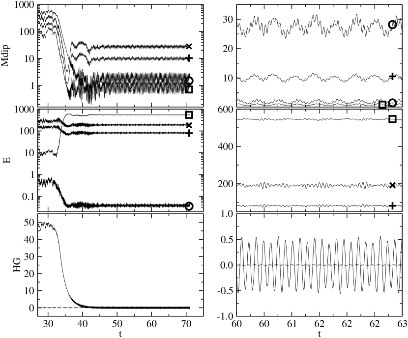
Figure 3: Time series of a dynamo solution in the case $\mathrm{P}=1$, $\mathrm{R}=10^{5}$, $\tau=2000$, $\mathrm{P}_{\mathrm{m}}=4.5$, $\eta=0.65$ and mixed velocity boundary conditions. The first row shows dipolar magnetic energy densities. The second row shows kinetic energy densities. The last row shows values of the mean dipolar, $H_{1}^{0}$, and the mean quadrupolar, $H_{2}^{0}$, components in the spherical harmonic expansion of the magnetic field. The components $\overline{X}_{p}$ $\overline{X}_{t}$, $\widetilde{X}_{p}$, and $\widetilde{X}_{t}$ are indicated by circles, squares, plus signs and crosses attached to the respective curves, and $X$ stands for either $M$ or $E$. The coefficient $H_{1}^{0}$ is represented by a solid line and $H_{2}^{0}$ by a dashed line. The time series in the right column represent enlarged sections of the ones in the left column.

4 An attempt to model the solar magnetic cycle

It appears from the results presented in the preceding section that variations of the shell thickness alone are not sufficient to induce oscillations in dipolar dynamo solutions. It is known that dipolar oscillations may be excited in a variety of other situations (Busse & Simitev 2006). An oscillating dipolar solution can be found when a region in the parameter space is approached where the quadrupolar or the higher-multipole components of the magnetic field are not negligible. As these components are typically oscillatory, an oscillation in the dipolar parts is also excited. A region of multipolar dynamos may be approached, for instance, by reducing the value of the magnetic Prandtl number $\mathrm{P}_{\mathrm{m}}$, or by increasing the value of the Rayleigh number $\mathrm{R}$ or of the rotation parameter $\tau$. In all of these situations one finds that the increase of the differential rotation plays a crucial role in exciting the oscillations. The differential rotation may, of course, be enhanced much more readily by imposing a stress-free boundary condition for the velocity field. Thus, the suggestion of Goudard & Dormy (2008) to replace the no-slip condition on the outer spherical boundary by a stress-free one is well-justified. As these authors remark, the choice of mixed velocity boundary conditions may be argued also on physical grounds: the no-slip condition at the inner boundary mimics the solar tachocline (Tobias 2005) and the stress-free condition at the outer boundary mimics the solar photosphere.

Figure 4: Half a period of dipolar oscillations of the dynamo shown in Fig. 3. Each circle of the first column shows lines of constant $\overline{B_{\varphi}}$ in the left half and of $r\sin\theta\partial_{\theta}\overline{h}=$ const. in the right half. The second column shows meridional lines of constant $B_{r}$ at $r=r_{o}$. The third column shows meridional lines of constant $\overline{u}_{\varphi}$ in the left half and of $r\sin\theta\partial_{\theta}\overline{v}$ in the right half. Plots follow from top to bottom with a time step $\Delta t=0.021665$.

In Fig. 3 a dynamo simulation with mixed velocity boundary conditions is presented. After an interval of about 5 viscous diffusion times an abrupt transition in the nature of the dynamo solution occurs. The most notable signature of the transition is the decrease of the magnetic energy density by more than an order of magnitude. At the same time the kinetic energy increases twofold, mostly due to the increase in differential rotation. This is not surprising as the increase is promoted by two effects: first, by the removal of the no-slip condition and second, by the decrease of magnetic field which, now becomes too weak to effectively act as a brake on differential rotation. This latter effect has been reported in numerous other cases (Busse 2002, Simitev & Busse 2005).

More subtly, the transition is observed as a change in the relative contributions of magnetic energy components. The mean poloidal dipolar magnetic energy $\overline{M}_{p}$ is no longer the dominant component and is overcome by the fluctuating parts of the magnetic energy. In this respect the transition is similar to the transition between Mean Dipolar (MD) and Fluctuating Dipolar (FD) dynamos recently reported by Simitev & Busse (2009).

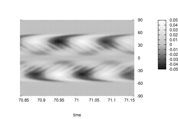
Figure 5: A butterfly diagram for the case shown in Figs. 3 and 4, i.e. the value of $r\partial_{\theta}\overline{g}$ at $r=r_{o}-0.05$ as a function of time and latitude.

The temporal behavior of the dynamo changes dramatically after the transition as well. In particular, it exhibits nearly periodic dipolar oscillations. These are evident in the right-hand side of Fig. 3 and even better in the oscillations of the spherical harmonic coefficient $H_{1}^{0}$ describing the contribution of the axial dipole in the solution. It is also remarkable that the quadrupolar coefficient $H_{2}^{0}$ remains much weaker than in corresponding oscillations in thick shell dynamos. A sequence of snapshots equidistant in time is shown in Fig. 4 in order to visualize half a period of oscillation. Except for the sign the plots shown in the last row closely resemble the ones in the first row confirming thus the near perfect periodicity of the oscillation. A polarity reversal of the magnetic field occurs during the cycle and is evident both in Fig. 4 and in the change of sign of $H_{1}^{0}$ in Fig. 3. This cyclic behavior is sustained for over 25 viscous diffusion times although it appears from the right-hand side of Fig. 3 that a weak modulation with a second frequency is also present. Finally, we remark that the oscillations appear to be well-described by the Parker wave linear analysis presented in Busse & Simitev (2006), in that the period of oscillation $T=0.12996$ is well approximated by the expression

$$T\approx\left(P_{m}\frac{\pi}{3}\langle\check{\mbox{\boldmath$v$}}\cdot\nabla\times\check{\mbox{\boldmath$v$}}\rangle\sqrt{2\overline{E_{t}}}\right)^{-1/2}$$

which in this case yields 0.11036.

In order to stress the similarity with the solar magnetic activity we present in Fig. 5 a butterfly diagram of the simulation, where the cyclic behavior and the propagation of magnetic features from high latitudes toward the equator is also visible.

5 Discussion and outlook

We have confirmed the finding of Goudard & Dormy (2008) of a sharp transition from a dynamo dominated by a non-oscillatory dipolar magnetic field to a nearly perfect oscillatory dynamo with a weaker dipole. We have related this transition to corresponding transitions from dynamos with a strong nearly steady dipole to oscillatory dynamos in thick shells. The introduction of a stress-free boundary condition at the outer spherical surface rather than the reduction of the shell thickness appears to be essential for the transition. It is of interest to note that the oscillations of thin shell dynamos are much more purely dipolar than those found in thick shells.

It is tempting to compare the oscillatory dipolar dynamo of section 3 to the magnetic activity of the Sun. A notable difference with the Sun is the profile of differential rotation of the solution which has the form of a nearly constant angular velocity on cylinders. Although this profile, when mapped to the surface $r=r_{o}$, reproduces qualitatively the rotation of the solar surface, the differences in radial direction are significant.

This is not surprising in view of the strong change of density throughout the solar convection zone caused by compressibility which has not been taken into account in our simple model. In addition the scales of turbulence are far from being resolved. This emphasizes the need to explore the parameter space of the problem in further detail.

We gratefully acknowledge support from CTR and NASA which made our visit to Stanford possible. The numerical calculations reported in this paper were carried out using the computer resources of the School of Mathematics and Statistics of the University of Glasgow, and the UK MHD supercomputer at the University of St. Andrews, UK.

References

- [Busse, 1970] Busse, F.H. 1970 Differential rotation in stellar convection zones Astrophys. J. 159 629-639.
- [Busse, 2002] Busse, F.H 2002 Convective flows in rapidly rotating spheres and their dynamo action Phys Fluids 14 (4) 1301.
- [Busse & Simitev, 2006] Busse, F.H. & Simitev, R. 2006 Parameter dependences of convection driven dynamos in rotating spherical fluid shells Geophys. Astrophys. Fluid Dyn. 100(4-5) 341.
- [Brandenburg & Subramanian, 2005] Brandenburg, A. & Subramanian, K. Astrophysical magnetic fields and nonlinear dynamo theory. Physics Reports, 417, 1.
- [Browning, 2007] Browning, M., Brun, A.S., Miesch, M. & Toomre, J. 2007 Dynamo action in simulations of penetrative solar convection with an imposed tachocline Astronom. Notes 328 1002.
- [Brun & Toomre, 2002] Brun, A. S. & Toomre, J. 2002 Turbulent convection under the influence of rotation: sustaining a strong differential rotation Astrophys. J. 570 865.
- [Christensen et al., 2001] Christensen, U.R., Aubert, J., Cardin P., et al. 2001 A numerical dynamo benchmark Phys. Earth Planet. Inter. 128 25.
- [Goudard & Dormy, 2008] Goudard, L. & Dormy, E. 2008 Relations between the dynamo region geometry and the magnetic behavior of stars and planets EPL 85 59001.
- [Rüdiger & Hollerbach, 2004] Rüdiger, G. & Hollerbach, R. 2004 Magnetic Universe: Geophysical And Astrophysical Dynamo Theory, Wiley
- [Schou et al., 1998] Schou, J., Antia, H., Basu, S., et al. 1998 Helioseismic studies of differential rotation in the solar envelope by the solar oscillations investigation using the Michelson Doppler Imager Astrophys. J. 505 390-417.
- [Simitev & Busse, 2005] Simitev, R. & Busse, F.H. 2005 Prandtl number dependence of convection driven dynamos in rotating spherical fluid shells J. Fluid Mech. 532 365.
- [Simitev & Busse, 2009] Simitev, R. & Busse, F.H. 2009 Bistability and hysteresis of dipolar dynamos generated by turbulent convection in rotating spherical shells EPL 85 19001.
- [Tilgner, 1999] Tilgner, A. 1999 Spectral methods for the simulation of incompressible flows in spherical shells Int. J. Num. Meth. Fluids 30 (6) 713.
- [Tobias, 2005] Tobias, S. 2005 The solar tachocline: Formation, stability and its role in the solar dynamo, pp. 193-233 in Fluid Dynamics and Dynamos in Astrophysics and Geophysics, A.M.Soward, C.A.Jones, D.W.Hughes, N.O.Weiss (eds.), CRC Press.