MRI-driven Accretion onto Magnetized stars: Axisymmetric MHD Simulations

Abstract

We present the first results of a global axisymmetric simulation of accretion onto rotating magnetized stars from a turbulent accretion disk, where the turbulence is driven by the magnetorotational instability (MRI). Long-lasting accretion is observed for several thousand rotation periods of the inner part of the disc. The angular momentum is transported outward by the magnetic stress of the turbulent flow with a rate corresponding to a Shakura-Sunyaev viscosity parameter $\alpha\approx 0.01-0.04$. Close to the star the disk is stopped by the magnetic pressure of the magnetosphere. The subsequent evolution depends on the orientation of the poloidal field in the disk relative to that of the star at the disk-magnetosphere boundary. If fields have the same polarity, then the magnetic flux is accumulated at the boundary and blocks the accretion which leads to the accumulation of matter at the boundary. Subsequently, this matter accretes to the star in outburst before accumulating again. Hence, the cycling, ‘bursty’ accretion is observed. The magnetic stress is enhanced at the boundary, leading to the enhanced accretion rate. If the disc and stellar fields have opposite polarity, then the field reconnection enhances the penetration of the disk matter towards the deeper field lines of the magnetosphere. However, the magnetic stress at the boundary is lower due to the field reconnection. This decreases the accretion rate and leads to smoother accretion at a lower rate. Test simulations show that in the case of higher accretion rate corresponding to $\alpha=0.05-0.1$, accretion is bursty in cases of both polarities. On the other hand, at much lower accretion rates corresponding to $\alpha<0.01$, accretion is not bursty in any of these cases. We conclude that the episodic, bursty accretion is expected during periods of higher accretion rates in the disc, and in some cases it may alternate between bursty and smooth accretion, if the disk brings the poloidal field of alternating polarity. We find that a rotating, magnetically-dominated corona forms above and below the disk, and that it slowly expands outward, driven by the magnetic force.

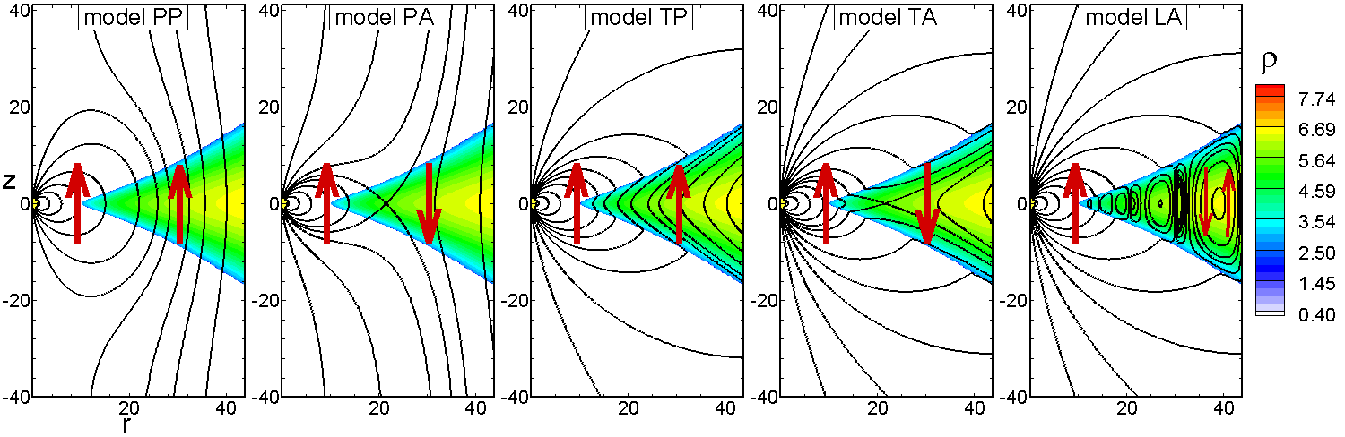
Figure 1: Initial distribution of the magnetic field used in different models. The dipole magnetic field of the star is fixed at $\widetilde{\mu}=20$, but the field distribution in the disc is different. From left to right: the field in the disc is vertical (parallel to the $z-$axis) and has the same direction as the magnetic field of the star at the disc-magnetosphere boundary (model VP20); same but for the opposite direction of the field in the disc (antiparallel case, model VA20); tapered field with $z-$component parallel to the field of the star (model TP20); tapered field with antiparallel field (model TA20); loops in the disc where the inner loop field is parallel to the star’s field (model LP20).

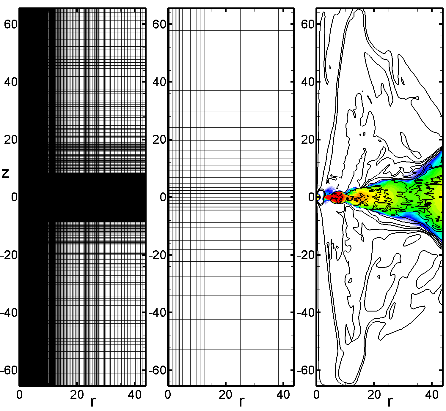
Figure 2: Left panel: The grid used in simulations; Middle panel: same grid, but rarefied by a factor of 10. Right panel: Sample simulation run shows the density distribution and selected field lines at the end of a long simulation run in model TP20 at $t=3000$.

1 Introduction

The magnetorotational instability (MRI) is the likely origin of turbulent stress in accretion disks around black holes and stars (e.g., Balbus & Hawley 1991; Balbus & Hawley 1998). MRI-driven accretion has been observed in a number of local and global axisymmetric and 3D MHD simulations (e.g., Hawley et al. 1995; Stone et al. 1996; Gammie & Menou 1998; Stone & Pringle 2001; Hawley 2000; Hawley et al. 2001; Hawley & Krolik 2002; Beckwith, et al. 2009). In these simulations the central object is a black hole. However, there are many stars which have dynamically important magnetic fields. These include young, Classical T Tauri stars (hereafter CTTSs; e.g., Bouvier et al. 2005), some types of white dwarfs, and neutron stars in binary systems (e.g., Warner 2004; Van der Klis 2000). In these stars, the magnetic field is strong enough to stop the disk at radii larger than the radius of the star. Many observational properties are determined by the processes at the disk-magnetosphere boundary.

The disk-magnetosphere interaction in the case of laminar (non-turbulent) flow in the disk has been investigated earlier in both axisymmetric (e.g., Miller & Stone 1997; Goodson et al. 1997; Goodson et al. 1999; Romanova et al. 2002; Bessolaz et al. 2008) and global 3D MHD simulations (Romanova et al. 2003; Romanova et al. 2004; Kulkarni & Romanova 2005; Long et al. 2008). The laminar flow in the disc is modeled with the $\alpha-$viscosity prescription (Shakura & Sunyaev 1973). Similarly, the $\alpha-$type magnetic diffusivity has been included in a number of studies. Heretofore, accretion due to turbulent, MRI-driven discs has not been studied.

Here, we present the results of the first axisymmetric simulations of MRI-driven accretion onto magnetized stars. In these simulations we were able to use a very high grid resolution and perform very long runs. Results for global 3D simulations will be discussed in a separate paper (Romanova et al., 2011). Accretion onto rapidly rotating stars will be described in Ustyugova et al. (2011). Here, we consider the case of slowly rotating stars.

Model	config.	direction	$B_{d}$	$\tilde{\mu}$	$t/P_{mid}$
VP30	vertical	parallel	+0.002	30	19
VA30	vertical	antipar.	– 0.002	30	14
TP30	tapered	parallel	+0.002	30	19
TA30	tapered	antipar.	– 0.002	30	14
VP20	vertical	parallel	+0.002	20	13
VA20	vertical	antipar.	– 0.002	20	14
TP20	tapered	parallel	+0.002	20	30
TA20	tapered	antipar.	– 0.002	20	17
LP20	loops	parallel	+0.002	20	13
LA20	loops	antipar.	– 0.002	20	34
TP20+B001	tapered	parallel	+0.001	20	12
TA20-B005	tapered	antipar.	– 0.005	20	33
TP10	tapered	parallel	+0.002	10	14
TA10	tapered	antipar.	– 0.002	10	16
TP5	tapered	parallel	+0.002	5	23
TA5	tapered	antipar.	– 0.002	5	13
TP2	tapered	parallel	+0.002	2	7
TA2	tapered	antipar.	– 0.002	2	13

Table 1: The Table describes the main simulation models, where the first letter in the model name stands for the field configuration: ‘V’ - vertical field, ‘T’ - tapered field, ‘L’ - looped field. The second letter stands for the mutual directions of the magnetic fields of the disc and the star: ‘P’ - parallel and ‘A’ - antiparallel. The number at the end of the name shows the value of the dimensionless magnetic moment $\tilde{\mu}$. The Table also shows the $z-$component of the seed magnetic field in the disc, $B_{d}$, and the duration of simulations in periods of rotation $P_{\rm mid}$ at the grid center, $r=22$ ($P_{\rm mid}=103P_{0}$).

2 Theoretical background

The magnetorotational instability (MRI) arises under conditions where a weak magnetic field threads the disc. Below, we briefly summarize the condition for the onset of the MRI instability (Balbus & Hawley 1991) for a simple case where an axial magnetic field $B_{0}\hat{\bf z}$ threads a Keplerian disc which rotates with angular rate $\Omega=(GM/r^{3})^{1/2}$ where $M$ is the mass of the central object. For axisymmetric perturbations of the disc with $\delta{\bf v}=[\delta v_{r}(z,t),\delta v_{\phi}(z,t),0]$ and $\delta{\bf B}=[\delta B_{r}(z,t),\delta B_{\phi}(z,t),0]$ and for perturbations proportional to $\exp(ik_{z}z-i\omega t)$, one finds the dispersion relation

$$\omega_{\pm}^{2}=(k_{z}v_{A})^{2}+{1\over 2}\kappa_{r}^{2}\pm\left[{1\over 4}\kappa_{r}^{4}+4(k_{z}v_{A}\Omega)^{2}\right]^{1/2}~{},$$ (1)

where $v_{A}\equiv B_{0}/\sqrt{4\pi\rho}$ is the Alfvén velocity and $\kappa_{r}\equiv[4\Omega^{2}+2r\Omega d\Omega/dr]^{1/2}$ is the radial epicyclic frequency of the disc. In order for the perturbation to fit within the vertical extent of the disc one needs $k_{z}h\gtrsim 1$, where $h=c_{s}/\Omega$ is the half-thickness of the disc and $c_{s}$ is the isothermal sound speed in the disc. For most conditions the disc is thin with $h\ll r$, or $c_{s}\ll r\Omega$.

Evidently, there can be instability if $\omega_{-}^{2}<0$ which happens if $(kv_{A})^{2}<-2r\Omega d\Omega/dr$. For a Keplerian disc this corresponds to $(kv_{A})^{2}<3\Omega^{2}$. Therefore, the above-mentioned condition that $k_{z}h\gtrsim 1$ implies that the instability occurs only for $v_{A}<c_{s}$, or

$$\beta\equiv{2c_{s}^{2}\over v_{A}^{2}}>1~{}.$$ (2)

Note that $\beta$ is based on the initial vertical magnetic field, $B_{0}$. As a result of the instability the magnetic field may grow to values much larger than $B_{0}$. The maximum value of the growth rate is $\Im(\omega)_{\rm max}=3\Omega/4$, and it occurs for $k_{\rm max}=(15/16)^{1/2}\Omega/v_{A}$. For $\beta<1$ the perturbation does not fit inside the disc and there is stability. As $\beta$ increases from unity (weaker magnetic field) the maximum growth rate stays the same but the wavelength of the perturbation gets shorter ($\propto\beta^{-1/2}$). Of course, for sufficiently small wavelengths the damping due to numerical viscosity ($\sim\nu_{\rm num}k^{2}$) will be larger than the MRI growth rate. To generate MRI-driven accretion in numerical simulations, one should have large enough $\beta$ in the disc so as to have instability, and at the same time high enough grid resolution to avoid the damping of small wavelengths.

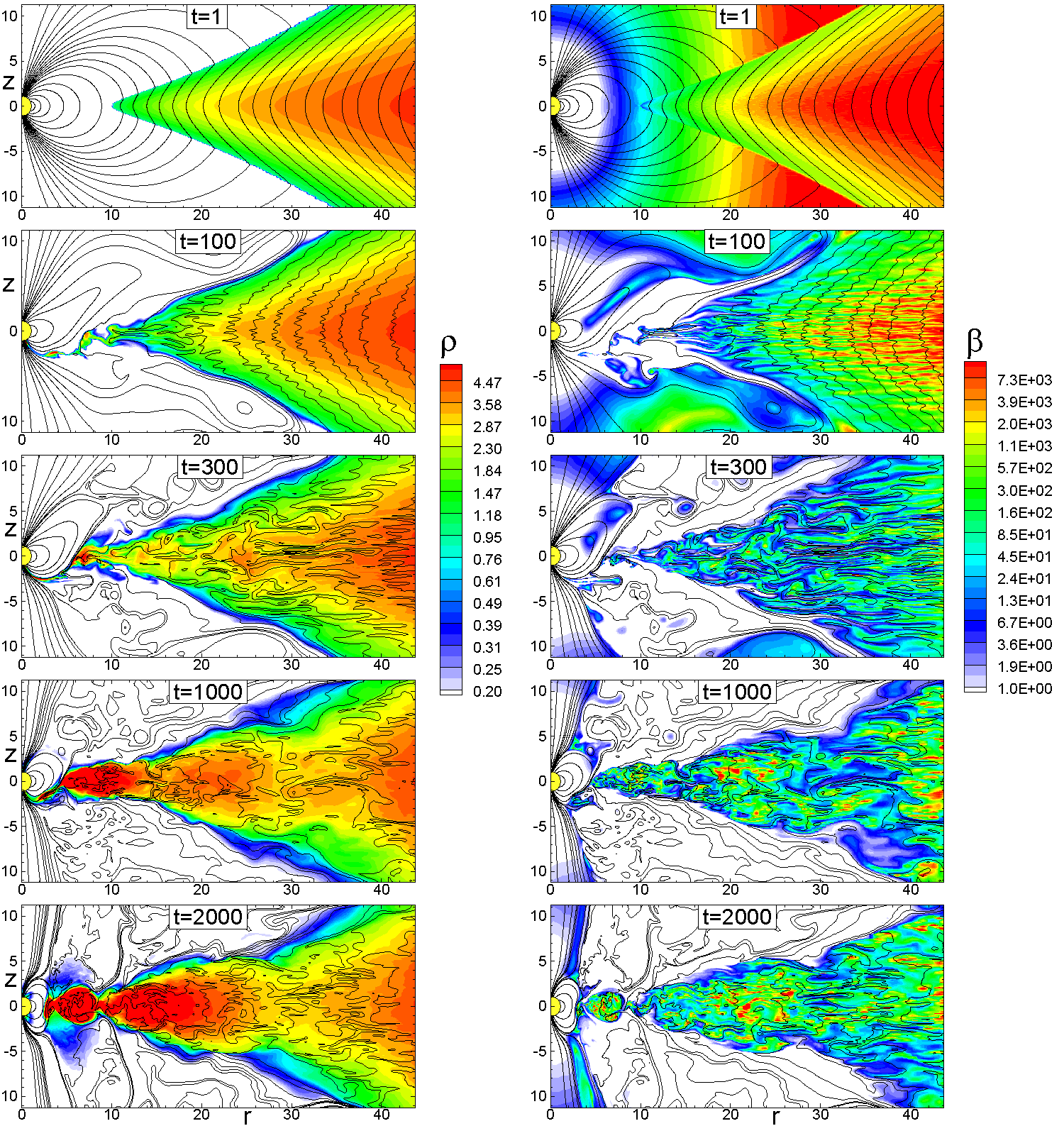
Figure 3: MRI-driven accretion at different times for model TP30. Left panels: The background shows the density and the lines are poloidal field lines. Right panels: The background shows the plasma parameter $\beta=8\pi P_{m}/B^{2}$, where $P_{m}$ is matter pressure.

3 Simulations of MRI instability

3.1 The problem setup

We investigate MRI-driven accretion onto a rotating star with a dipole magnetic field. The field lines are frozen into the stellar surface, and initially, they thread the entire simulation region, including the disc. The disc is dense and cold while the corona is $10^{3}$ times hotter and $10^{3}$ times less dense. The disc rotates with the Keplerian velocity at the beginning of the simulation. The corona also rotates with Keplerian velocities at cylindrical radii corresponding to the rotation of the disc. This helps to avoid the build-up of an initial discontinuity of the magnetic field at the disc-magnetosphere boundary. We derive the initial distribution of density and pressure in the disc and corona by balancing the gravitational, centrifugal and pressure gradient forces (see Sec. A.4 for details). The initial inner disc radius is set to $r=10$ (in units of stellar radius, $R_{0}$; see Sec. A.4 for the full description of reference units). The star rotates slowly with an angular velocity corresponding to a corotation radius ($r_{\rm cor}=(GM/\Omega_{*}^{2})^{1/3}$) of $10$ (in dimensionless units).

A small seed poloidal field with $z-$component $B_{d}$ has been added to the disc, which is necessary for the initial excitation of the MRI-driven turbulence. We considered three types of initial configurations:

• Vertical field(‘V-’type models): The field is vertical (that is, parallel to the $z-$axis), has a value of $B_{d}$ and is homogeneous in space. The alignment of the field may be parallel or antiparallel to the star’s magnetic field at the disc-magnetosphere boundary (see two left panels in Fig. 1).

• Tapered field (‘T-’type models): An initially vertical field tapered in such a way that the magnetic flux is restricted to lie within the disc . The magnetic flux inside a disc with half-thickness $h$ (at $|z|\leq h$) is determined by:

  $$\Psi=\frac{B_{d}r^{2}}{2}\cos\bigg{(}\pi\frac{z}{2h}\bigg{)},~{}~{}~{}~{}h=\sqrt{\bigg{(}\frac{GM}{\Phi_{c}(r)-E}\bigg{)}^{2}-r^{2}},$$ (3)

  where $\Phi_{c}(r)=\kappa GM/r$, $E$ is the constant of integration in the initial equilibrium equation (see Sec. A.4). Fig. 1 (3rd and 4th panels from the left) shows cases of parallel (model ‘TP’) and antiparallel (model ‘TA’) fields.

• Looped field (‘L-’type models): The magnetic flux inside a disc with half-thickness $h$ is determined by:

  $$\Psi=\frac{B_{d}r^{2}}{2}\cos\bigg{(}a\pi\frac{z}{2h}\bigg{)}\sin\bigg{(}b\pi\frac{r-r_{d}}{r_{out}-r_{d}}\bigg{)}~{},~{}$$ (4)

  where parameters $a$ and $b$ determine the number of loops in the vertical and horizontal directions, $r_{out}$ is the radius of the external boundary, and $r_{d}$ is the inner disc radius.

  We experimented with different numbers of loops with values of $Nr_{\rm loops}\times Nz_{\rm loops}$ ranging from $3\times 1$ to $7\times 5$, and concluded that the case with the smaller number of loops ($3\times 1$) is sufficient for exciting the turbulence, while the cases with a larger number of loops do not have advantages. The total poloidal flux is not zero, and hence we have two cases where the averaged field in the disc is parallel (model ‘LP’) or antiparallel (model ‘LA’) to the field of the star (see an example for ‘LP-’type configuration at the right panel of Fig. 1).

We solve the ideal MHD equations (see Sec. A.1), given axisymmetric conditions, in cylindrical coordinates using a Godunov-type code (see Sec. A.3). The grid is of high resolution with compression towards the disc midplane and towards the $z-$axis with the goal of having a larger number of the grid-points in the disc and near the star (see Fig. 2). After compression, a typical grid has $N_{r}=270$ cells in the radial direction and $N_{z}=432$ cells in the axial direction. The number of grids covering the disc in the vertical direction (in the middle of the disc) is about 200. The grid also has sufficiently high resolution in the $r-$direction. The simulation region is stretched in the $z-$direction to allow for matter flow in the corona.

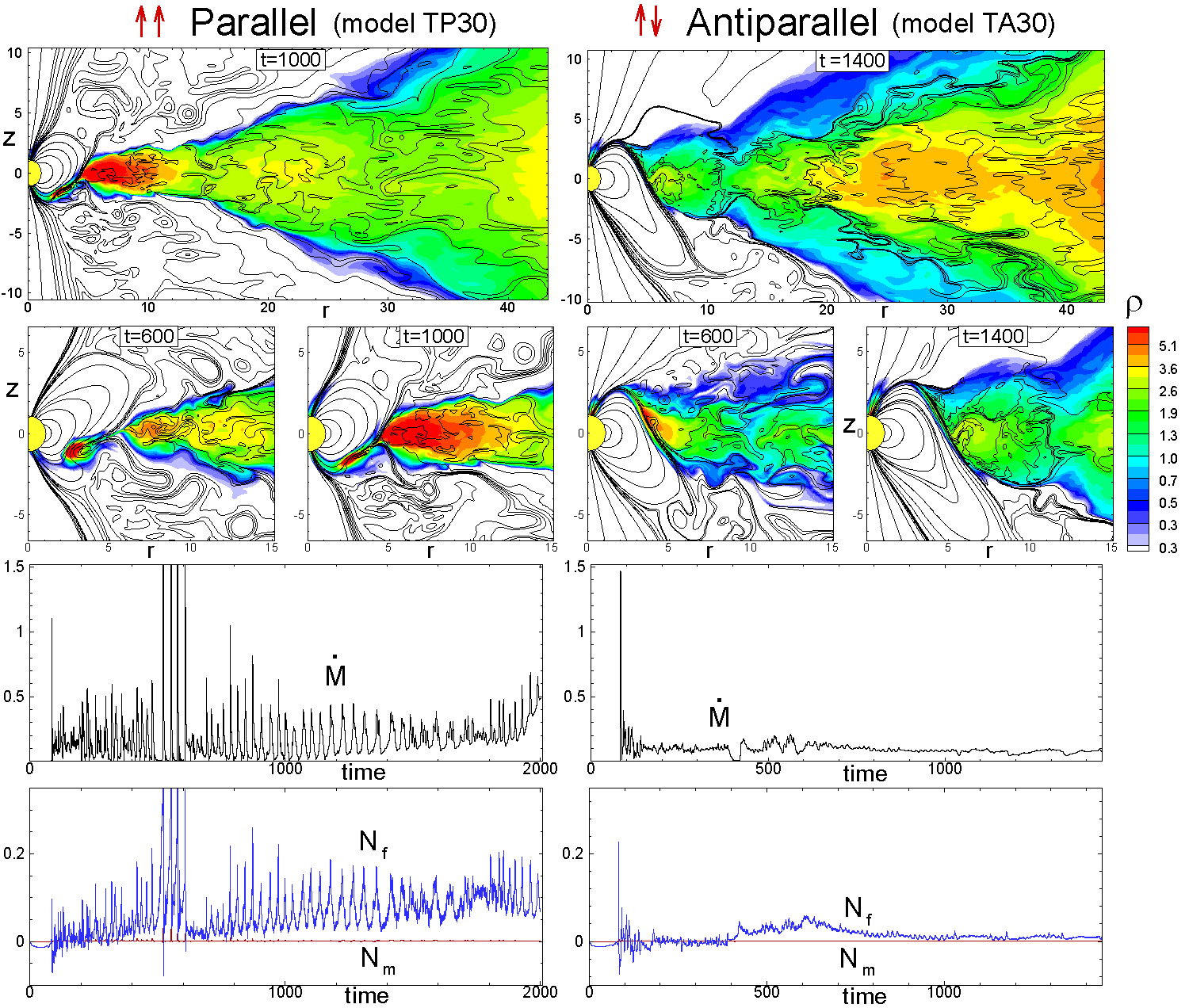
Figure 4: Left panels: MRI-driven accretion at different moments of time for model TP30 where the seed magnetic field in the disc is parallel to that of the star at the disc-magnetosphere boundary. The background shows the density, lines show the poloidal field lines. Right panels: Same but for the case of antiparallel fields. The top row shows the flow in the whole simulation region at two moments of time $t=600$ and $1000$. The next row shows matter flow near the star for the same cases. The 3rd and 4th rows show the temporal evolution of matter flux onto the star $\dot{M}$ and torque on the star associated with matter, $N_{m}$, and the magnetic field, $N_{f}$ for corresponding models.

3.2 The parameters in different simulation runs

We ran various simulations given different initial configurations of the field within the disc (see Fig. 1 and Tab. 1). We observed that similar MRI-driven turbulence develops in all cases. We chose the tapered field configuration as a base, because it is the simplest after the vertical field configuration, but most of its magnetic flux is confined within the disc.

The strength of the MRI-driven turbulence and the subsequent accretion rate depends on the value of the seed poloidal field in the disc, $B_{d}$. We observed that if the field is strong $B_{d}\gtrsim 0.01$ (see Sec. A.2 for reference units), the accretion rate is very high, and also the long wavelength modes dominate. If the field is weak, $B_{d}\lesssim 0.0005$) then the accretion rate is very low. We chose the intermediate value $B_{z}=\pm 0.002$ for almost all simulation runs. We also performed test runs at higher ($B_{d}=-0.005$) and lower ($B_{d}=0.001$) fields. The result also depends on the orientation of the seed field in the disc. Note that the field of the star at the disc-magnetosphere boundary is positive, and hence the plus sign for $B_{d}$ means that the fields have the same direction.

Our initial setup for the disc and corona differs from the commonly used setup for accretion to black holes, where the matter is initially confined inside a thick torus of constant specific angular momentum. The torus gradually evolves into the disc-type structure (e.g., Hawley 2000). In contrast, our disc rotates with Keplerian velocity and has a quasi-equilibrium density distribution from the beginning of simulations (see Sec. A.4). In addition, matter with a seed field can flow inward from the side boundary, and this allows for longer simulation runs (see Sec. A.5).

We also performed simulations for different sizes of the magnetospheres which are determined by the dimensionless parameter $\tilde{\mu}$ (see Tab. 1 and Sec. 6).

3.3 Initial perturbations in the disc

Here, we use our dimensionless variables (see Sec. A.2) to estimate the number of MRI waves per thickness of the disc. The wavelength of most unstable, MRI-driven modes is given by $\lambda_{\rm MRI}\approx 2\pi{v_{A,z}}/{\Omega_{K}}$. The full thickness of the initially isothermal disc is $2h\approx{2c_{s}}/{\Omega_{K}}$, where $c_{s}=\sqrt{p/\rho}$ is the isothermal sound speed in the disc. Hence, the number of waves per thickness of the disc is $N_{\rm MRI}={2h}/{\lambda_{\rm MRI}}\approx{c_{s}}/{\pi v_{A,z}}$. In our simulations (in dimensionless units, see Sec. A.2) $c_{s}=0.032$, the density in the disc is $\rho_{d}\approx 1$, the Alfvén velocity (based on the $B_{d}=0.002$ field) is $v_{A,z}={B_{d}}/{\sqrt{4\pi\rho_{d}}}\approx 5.7\times 10^{-4}$. Substituting these values into the initial formula, we obtain the number of waves per disc and also the plasma parameter $\beta$ :

$$N_{\rm MRI}=\frac{2h}{\lambda_{\rm MRI}}=17\bigg{(}\frac{0.002}{B_{d}}\bigg{)},$$ (5)

$$\beta\equiv{2c_{s}^{2}\over v_{A}^{2}}=6.2\times 10^{3}\bigg{(}\frac{0.002}{B_{d}}\bigg{)}^{2}~{}.$$ (6)

This value of $\beta$ corresponds approximately to the initial value of $\beta$ in the middle of the disc in our simulations. Below, we show the development of the MRI-driven turbulence for one of our models.

3.4 Development of MRI-driven turbulence in simulations

Here, we take one of our models (TP30) and show the development of the MRI-driven flow. We take the case of the largest magnetosphere (in our set) to investigate whether the large magnetosphere can hinder the development of turbulence or subsequent inward accretion towards the star.

When we imposed small random fluctuations of the angular velocity in the disc, the fluctuations grew. Fig. 3 (top panels) shows the distribution of density $\rho$ and $\beta$ at an early time ($t=1$). One can see that the density increases towards larger radii. In our initial conditions (see Sec. A.4), the density may either increase or decrease towards larger radii, and it is regulated by a coefficient in the initial, almost Keplerian, angular velocity distribution: $\Omega(r)=(1\pm 0.02)\Omega_{K}$, where the ‘$-$’ sign means the density increases outward. We chose this case for all our simulation runs because it corresponds to softer start-up conditions and the simulations last longer. Note that the initial distribution of the plasma parameter $\beta$ is not homogeneous: it varies between $\beta=20$ at the inner edge of the disc and $\beta=2\times 10^{4}$ at the outer edge. In the middle of the disc, at $r=22$, we have $\beta=3\times 10^{3}$ (which roughly corresponds to the value derived in the previous section). This strong initial variation in $\beta$ is associated with two factors: (1) the density increases towards larger radii; and (2) the initial magnetic field in the disc is a superposition of the strong dipole field that dominates at the inner regions of the disc, and the almost homogeneous seed initial field in the disc. The superposition of fields gives the field $B=0.01$ at the inner edge of the disc, $B=0.005$ in the middle (at $r=22$) and $B=0.002$ at the outer edge. Note that in the ‘torus’ initial conditions (e.g., Hawley 2000) the $\beta$ also varies across the torus, but not as much.

Later, we observed that the growth rate of the instabilities is on the time scale of Keplerian rotations. Fig. 3 (second row) shows the density and $\beta$ distributions at time $t=100$, which corresponds to one Keplerian rotation at $r=21$ (in the middle of the simulation region). One can see that channel modes developed at this and smaller radii. The number of modes per thickness of the disc expected from theory (see Eq. 5) is $N_{\rm MRI}\approx 5$ for the inner disc, $N_{\rm MRI}\approx 8-9$ for the middle of the disc and $N_{\rm MRI}=17$ for the outer disc. One can see that at this time, the instability already developed at the inner disc with few modes visible in the plot, and the correct number of modes have developed in the middle of the disc. The external regions show stretching of the initial perturbations.

The next row in Fig. 3 shows a later time, $t=300$, which corresponds to one Keplerian rotation at the outer edge of the disc $r\approx 44$. One can see that the channel modes have developed in the whole disc including the outer boundary. Again, the number of modes roughly corresponds to the predicted number $N_{\rm MRI}\approx 17$ for this value of the field. Note that recently developed channel modes in the outer part of the disc are very ordered, while those in the inner and middle parts of the disc start to be mixed.

At later times, $t>500$, the channel modes mix as a result of interacting with one another, as well as with turbulent matter that is not in channel streams. Recently, Latter et al. (2009) suggested that the ‘turbulent mixing’ is probably the main process which destroys the channel modes (and not the parasitic instabilities as suggested earlier, e.g. Goodman & Xu 1994). The bottom panels corresponding to $t=1000$ and $t=2000$ show that the flow in most of the disc is very well mixed and is turbulent. The isolated channel streams appear in different parts of the disc and propagate inward, but they do not determine the character of matter flow at the inner parts of the disc. Formation of isolated channels which transfer energy to the turbulent matter has been discussed by Latter et al. (2009). Most importantly, the turbulent flow dominates in the inner parts of the disc which are important for investigating the disc-magnetosphere interaction.

The left panels of Fig. 3 show that the density is gradually redistributed in such a way that the highest density is in the inner parts of the disc, which corresponds to a quasi-stationary disc equilibrium.

4 MRI-driven accretion in cases of parallel and antiparallel fields

Our simulations show that the disc-magnetosphere interaction depends on the orientation of the seed poloidal field in the disc. If at the disc-magnetosphere boundary the $B_{z}-$component of the disc field points in the same direction as the field of the star, then the field is enhanced at the boundary initially. Subsequently, the disc matter continues to bring the field of the same polarity. In the case of antiparallel fields, the field at the disc-magnetosphere boundary is weaker initially, and subsequently, disc matter brings in a field of the opposite polarity, and this influences matter flow in the inner disc and at the boundary. Below, we consider two specific models with parallel (TP30) and antiparallel (TA30) fields and discuss the results in detail.

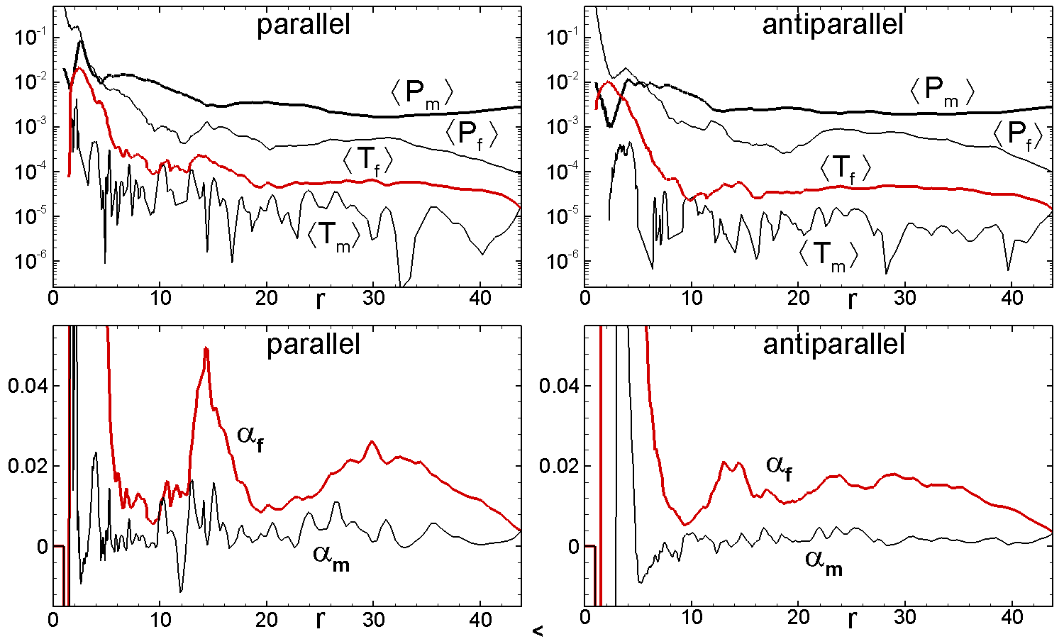
Figure 5: Top panels: Radial distribution of matter and magnetic pressure, $\langle{P_{m}}\rangle,\langle{P_{f}}\rangle$, and stresses, $\langle{T_{m}}\rangle,\langle{T_{f}}\rangle$ which were integrated across the disc, at time $t=1000$. Bottom panels: Same for $\alpha-$parameters associated with matter and magnetic stresses, $\alpha_{m},\alpha_{f}$. Left and right panels correspond to models TP30 (parallel fields) and TA30 (antiparallel fields), respectively.

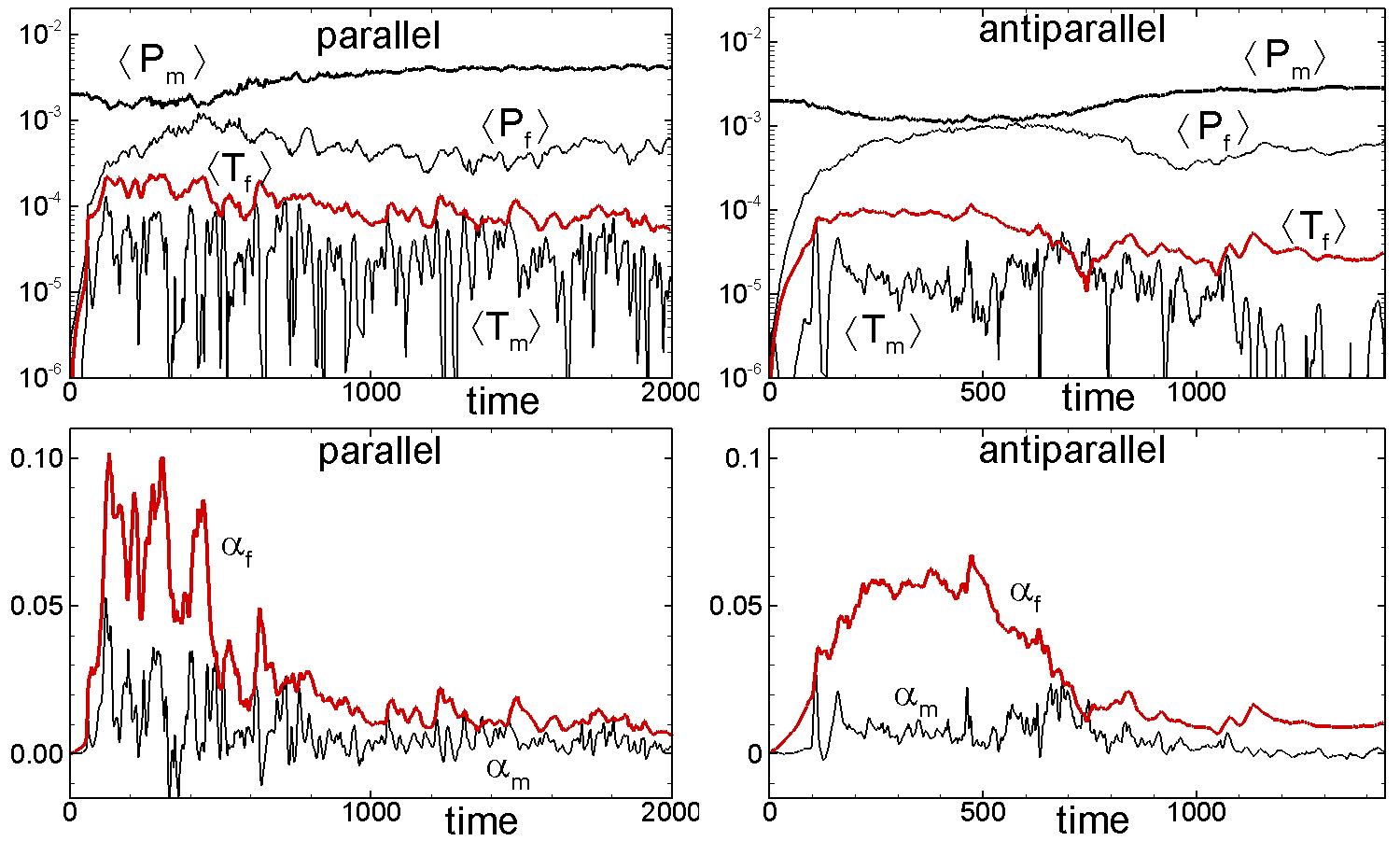
Figure 6: Top panels: Temporal evolution of matter and magnetic pressure, $\langle{P_{m}}\rangle,\langle{P_{f}}\rangle$, and stresses , $\langle{T_{m}}\rangle,\langle{T_{f}}\rangle$ taken at the radius $r=20$ and integrated across the disc. Bottom panels: Temporal variation of $\alpha-$parameters associated with matter and magnetic stresses, $\alpha_{m},\alpha_{f}$. Left and right panels correspond to models TP30 (parallel fields) and TA30 (antiparallel fields).

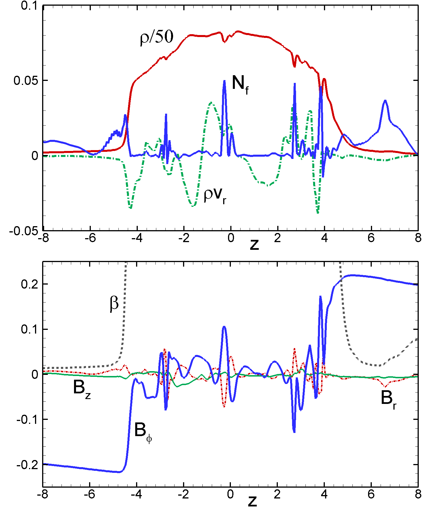
Figure 7: Top panel: Distribution of radial velocity $v_{r}$, specific matter flux $\rho v_{r}$, specific magnetic torque $N_{f}$ and the density $\rho$ across the disc at radius $r=20$ and time $t=1000$ in model TP30. The density is decreased by a factor of 50 for scaling, and $N_{f}$ is increased by a factor of 4. Bottom panel: same as above, but for three components of the magnetic field and plasma parameter $\beta=8\pi P_{m}/B^{2}$. The plasma parameter varies between small values outside the disc, up to $\beta>>1$ inside the disc.

4.1 Matter flow, matter flux and torque

We observed that in both models, MRI-driven turbulence develops in the disc and matter flows inward. The top rows of Fig. 4 show accretion on large and small scales at two times for model TP30 with parallel fields (left side of the plot) and model TA30 with antiparallel fields (right side). We observed that in both cases, the disc moves inward due to MRI-driven turbulence, but it is stopped by the magnetic pressure of the star. Then matter is lifted above the closed magnetosphere and accretes to the stellar surface in funnel streams. We observed that the closed magnetosphere initially expands towards one side, while matter accretes from the other side. Initial penetration of the disc matter through the closed magnetosphere is accompanied by strong reconnection events. Note that the disc is thicker in the case of antiparallel fields.

We calculated matter fluxes and torque at the surface of the star:

$$\dot{M}=\int d{\bf S}\cdot{\bf F}_{m}~{},\quad\quad{\bf F}_{m}=\rho{\bf v}_{p}~{},$$ (7)

$$N=\int d{\bf S}\cdot({\bf N}_{\rm m}+{\bf N}_{\rm f})~{},$$ (8)

where $d{\bf S}$ is the surface area element directed outward; ${\bf N}_{\rm m}$ and ${\bf N}_{\rm f}$ are torques associated with matter and the magnetic field:

$${\bf N}_{\rm m} = r\rho v_{\phi}{\bf v}_{p}~{},\quad\quad{\bf N}_{\rm f}=-r\frac{B_{\phi}{\bf B}_{p}}{4\pi}~{}.$$ (9)

Fig. 4 (bottom panels) shows that the matter fluxes are strikingly different in cases of parallel (left panels) and antiparallel (right panels) fields. In the case of parallel fields, matter accretes onto the star in bursts, whereas in the case of antiparallel fields the accretion is smooth (after the first burst) and is also at the lower level. We suggest that in the case of parallel fields, the magnetic flux accumulates at the disc-magnetosphere boundary and blocks accretion. Matter accumulates, and later finds a path towards the star. This leads to periods of low accretion rate (when accretion is blocked) and high accretion rate through a burst. For antiparallel fields fields of opposite polarity frequently reconnect at the disc-magnetosphere boundary, opening the path for smoother accretion. It is interesting to note that the ‘first burst’ is observed in both cases.

We calculated the torque exerted on the star by matter, $N_{m}$ and the field $N_{f}$. We observed that the magnetic torque is much larger than the material torque and it repeats the pattern of the matter flux, $\dot{M}$. The torque is positive (we changed the sign compared with the formulae Eq. 9 for convenience of illustration) so the accreting matter spins up the star. This is what we expect, because the star rotates slowly. The observed properties of the magnetic and material torques are similar to those observed in laminar, $\alpha-$discs (Romanova et al., 2002).

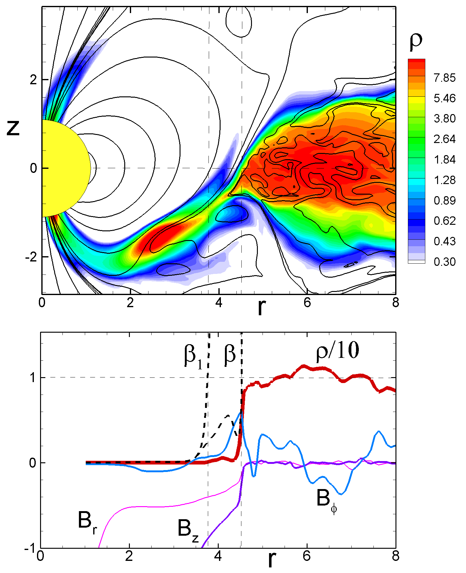
Figure 8: Top panel: close view of the funnel stream at $T=1000$ in model TP30. Bottom panel: radial distribution of density ($\rho$), angular velocity ($\Omega$), plasma parameters ($\beta$, $\beta_{1}$), azimuthal component of the field, $B_{\phi}$, and radial and z-components of the field ($B_{r}$, $B_{z}$). The density is multiplied by a factor of 0.1 for scaling.

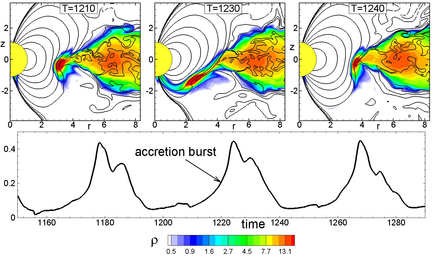
Figure 9: Top Panels: Matter flow before, during, and after the accretion event in model TP30, where the accretion rate enhancement is determined by the ‘push’ mechanism. The background shows the density and the lines are selected magnetic field lines. Bottom Panel: Matter flux onto the star during this accretion event, which is marked by an arrow.

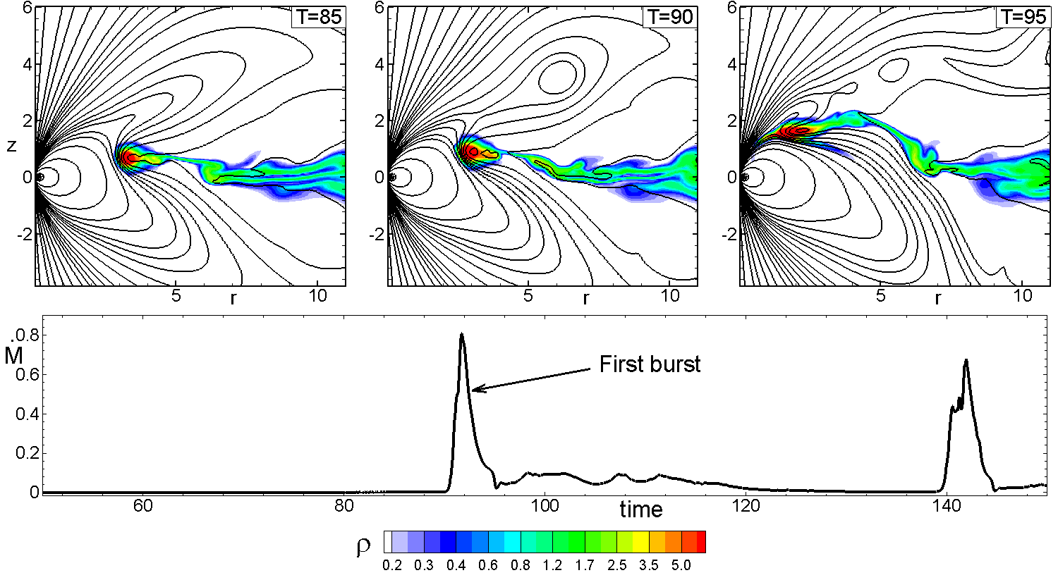
Figure 10: The figure shows an event of the ‘first burst’, where the initial stage of the disc penetration leads to reconnection of the significant magnetic flux of the external magnetosphere. An example is shown for model TP20.

4.2 Analysis of stresses and $\alpha-$parameters

Here we analyze the stresses acting inside the disc. We separate the disc from the low-density corona using one of the density levels, $\rho_{disc}=0.3$, which is typical for the boundary between the disc and corona. We integrate matter (subscript ‘m’) and magnetic (subscript ‘f’) stresses in the $z-$direction and obtain their distribution as a function of radius in the co-moving frame:

$$\langle{T_{m}}\rangle=\frac{1}{2h}\int dz\rho v_{r}v_{\phi}-\langle{\rho v_{r}}\rangle\langle{v_{\phi}}\rangle$$

$$\langle{T_{f}}\rangle=-\frac{1}{2h}\int dz\frac{B_{r}B_{\phi}}{4\pi}$$

where

$$\langle{v_{\phi}}\rangle=\frac{1}{M}\int dz\rho v_{\phi},~{}~{}\langle{\rho v_{r}}\rangle=\frac{1}{2h}\int dz\rho v_{r},$$

are averaged azimuthal velocity and matter flux, and $h=h(r)$ is the half-thickness of the disc.

The matter and magnetic pressure are

$$\langle{P_{m}}\rangle=\frac{1}{2h}\int dzP,~{}~{}~{}\langle{P_{f}}\rangle=\frac{1}{2h}\int dz\frac{B_{tot}^{2}}{8\pi}.$$

The standard $\alpha-$parameters associated with matter and magnetic stresses are:

$$\alpha_{m}=\frac{2}{3}\frac{\langle{T_{m}}\rangle}{\langle{P_{m}}\rangle},~{}~{}~{}\alpha_{f}=\frac{2}{3}\frac{\langle{T_{f}}\rangle}{\langle{P_{m}}\rangle}.$$

Fig. 5 shows the radial distribution of the magnetic and matter stresses, pressure, and corresponding $\alpha-$parameters for models TP30 and TA30. One can see that in model TP30 (see left panels) the magnetic stress $\langle{T_{f}}\rangle$ is about 10 times larger than matter stress and hence the magnetic stress determines the angular momentum transport. The matter pressure dominates over the magnetic pressure. The magnetic $\alpha-$parameter varies in the range of $\alpha_{f}\approx 0.01-0.05$, while the matter $\alpha-$parameter, $\alpha_{m}$, is $5-10$ times smaller. Hence, the angular momentum transport and inward accretion is determined by the magnetic stress. Note that the size of the stellar magnetosphere (magnetically-dominated region) is $r_{m}\approx 4-6R_{*}$, and this region should be excluded from our consideration, because we are only interested in the stresses in the disc.

The right panels of Fig. 5 show corresponding values for model TA30. In this model the seed poloidal field in the disc is antiparallel to the stellar field, and initial stress is somewhat smaller in the inner parts of the disc. We should note that in this case, the field in the disc is weaker than in the model TP30, because the oppositely-directed stellar field is subtracted from the disc field. This leads to smaller magnetic stress, which is still a few times larger than the matter stress. The magnetic pressure is smaller than the matter pressure in the majority of the disc. The magnetic alpha-parameter $\alpha_{f}$ is about 1.5 times larger than $\alpha_{m}$ and the magnetic field is responsible for the angular momentum transport.

In addition, we investigated variation of stresses and other variables in time. The $z-$averaged values are taken in the middle of the disc (at a radius $r=20$). Fig. 6 (top panels) shows that the magnetic $\alpha-$parameter ($\alpha_{f}$) is larger than the $\alpha_{m}$-parameter during the whole time, and hence the magnetic stress determines accretion. Both $\alpha$-parameters decrease with time. The value of $\alpha_{m}$ has a similar pattern, but at smaller values. The bottom panels of Fig. 6 show that all stresses and pressure values are quite steady with time on average, and only slightly decrease with time. Note that $\alpha_{f}$ and $\alpha_{m}$ decrease with time, but this is partially because the stresses gradually decrease with time and partially because the matter pressure $\langle{P_{m}}\rangle$ increases.

Results are shown up to $t=2000$ periods of rotation at the inner boundary ($r=1$), which corresponds to 20 periods of rotation at $r=22$.

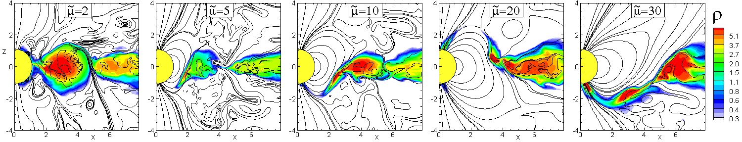
Figure 11: Sample plots for accretion onto stars with different magnetosphere sizes at time $t=700$. Parameter $\tilde{\mu}$ varies (from left to right) as $\tilde{\mu}=2,5,10,20,30$.

5 The disc-magnetosphere interaction

Here, we investigate in greater detail processes at the disc-magnetosphere boundary.

5.1 Where the disc stops

We take as an example the model TP30 and one of the moments in time when matter flows along the funnel towards the star. Fig. 8 (top panel) shows the inner part of the simulation region. One can see that the disc is stopped at some distance from the star and matter flows into the funnel stream. The conductivity is high, and some matter is dragged into the funnel stream. The matter energy-density is still higher than the magnetic energy in the funnel, but the magnetic field imposes some tension force, which acts in the direction opposite to the flow. This stress is released due to reconnection inside the funnel stream. Such mini-reconnection events are always observed in the funnel streams, in particular in cases of parallel fields.

The bottom panel of Fig. 8 shows a linear distribution of different variables in the equatorial plane. One can see that at the disc-magnetosphere boundary the density $\rho$ drops from high values in the disc to very low values in the magnetosphere. The $B_{\phi}$ component of the field dominates inside the disc, but drops at the boundary. The $B_{z}$ and $B_{r}$ components are very small in the disc, but strongly increase in the region of the magnetically-dominated magnetosphere. Note that the $B_{r}-$component is quite large because the magnetosphere is pushed upward by the funnel stream. Fig. 8 also shows the equatorial distribution of plasma parameter $\beta=8\pi P_{m}/B^{2}$ and the modified parameter $\beta_{1}$ based on the total material stress:

$$\beta_{1}=\frac{P_{m}+\rho v^{2}}{B^{2}/8\pi}~{}.$$ (10)

One can see that the disc-magnetosphere boundary is located between the radii where $\beta=1$ and $\beta_{1}=1$. This is in accord with earlier simulations of $\alpha-$discs, where the inner boundary usually coincides with $\beta_{1}=1$ surface (e.g., Romanova et al. 2002, Romanova et al. 2004), while the funnel starts at $\beta=1$ (Bessolaz et al., 2008).

However, the disc-magnetosphere interaction in the case of turbulent discs shows many features which are different from those observed in the case of $\alpha-$discs. One of the differences is that in the modeling of accretion from $\alpha-$discs the diffusivity was taken to be of the same order as viscosity, and both can be small, $\alpha\sim 0.01-0.02$ (like, e.g., in Romanova et al. 2002, 2003), or larger, $\alpha=0.1$ (e.g. Bessolaz et al. 2008), and in both cases matter smoothly flows from the disc to the star. The MRI-driven turbulence provides viscosity at the level of $\alpha\sim 0.01-0.1$, but it does not provide the cross-field diffusivity. This is why we often have the situation that accretion is blocked by the magnetic flux, and it leads to strong variability. In addition, in cases of one or another polarity in the disc, the variability is different, as discussed in Sec. 4.1 and subsequent sections.

5.2 The ‘push’ mechanism of accretion and oscillations

We often see strong oscillations in the light-curves. Usually, oscillations are connected with an accumulation of magnetic flux at the boundary, which generally occurs in cases where the seed magnetic field has the same polarity as the magnetic field of the star (cases of parallel fields).

Fig. 9 shows one of the episodes of enhanced accretion observed in model TP30 (the case of parallel fields, see Fig. 4). The left panel of Fig. 9 shows that matter accumulates at the disc-magnetosphere boundary. The magnetic field carried by the inner disc has the same polarity as the stellar field, and hence they do not reconnect. Matter bends the magnetosphere in such a way that accretion towards the star through the funnel stream becomes impossible. However, when ‘enough’ matter accumulates, it starts pushing the magnetosphere forward, so that accretion becomes possible (see middle panel). This happens because the gravity force becomes larger than the tension force associated with bending. After downloading matter onto the surface of the star, the magnetosphere expands and accretion is blocked again by the negative inclination of the field lines (see right panel). The bottom panel shows the corresponding burst in the accretion rate. We call this mechanism the ’push’ mechanism. It is responsible for the majority of bursts seen in the light-curve of model TP30 (see Fig. 4, left panels) and in many other cases shown below.

5.3 The ‘First Burst’

The accretion rate in the disc may vary with time. If accretion rate is relatively low, then the magnetosphere expands and the disc is at larger radii. When accretion rate increases after a period of low accretion rate, the inner disc moves forward and compresses the magnetic flux of the star. Finally, it stops at the point where material and matter stresses are comparable. However, the compressed magnetic flux blocks accretion. In MRI simulations the diffusivity is very low, and the disc matter cannot easily penetrate through all this flux.

Initially, our simulations corresponded to such a situation. We observed that matter accumulates in the inner disc (see Fig. 10, left panel), then moves towards the star, forcing all the external flux to reconnect (see middle and right panels). This event leads to a burst in the accretion rate (see bottom panel). In addition, one can expect strong X-ray flare associated with reconnection of significant magnetic flux.

The phenomenon of the first burst corresponds to our initial stage of evolution. However, such an initial burst is expected in stars with strongly varying accretion rate. Note that the ‘first burst’ is expected in cases of both parallel and antiparallel fields (see Fig. 4).

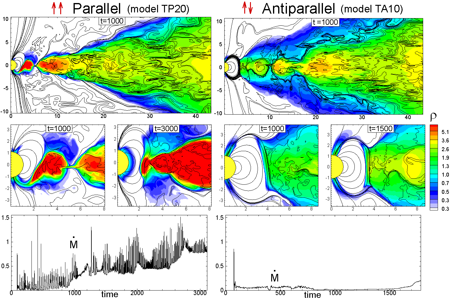
Figure 12: Accretion onto a star with a large magnetosphere (models TP20 and TA20) in cases of parallel (left panels) and antiparallel (right panels) fields. Bottom panels show accretion rate onto the star.

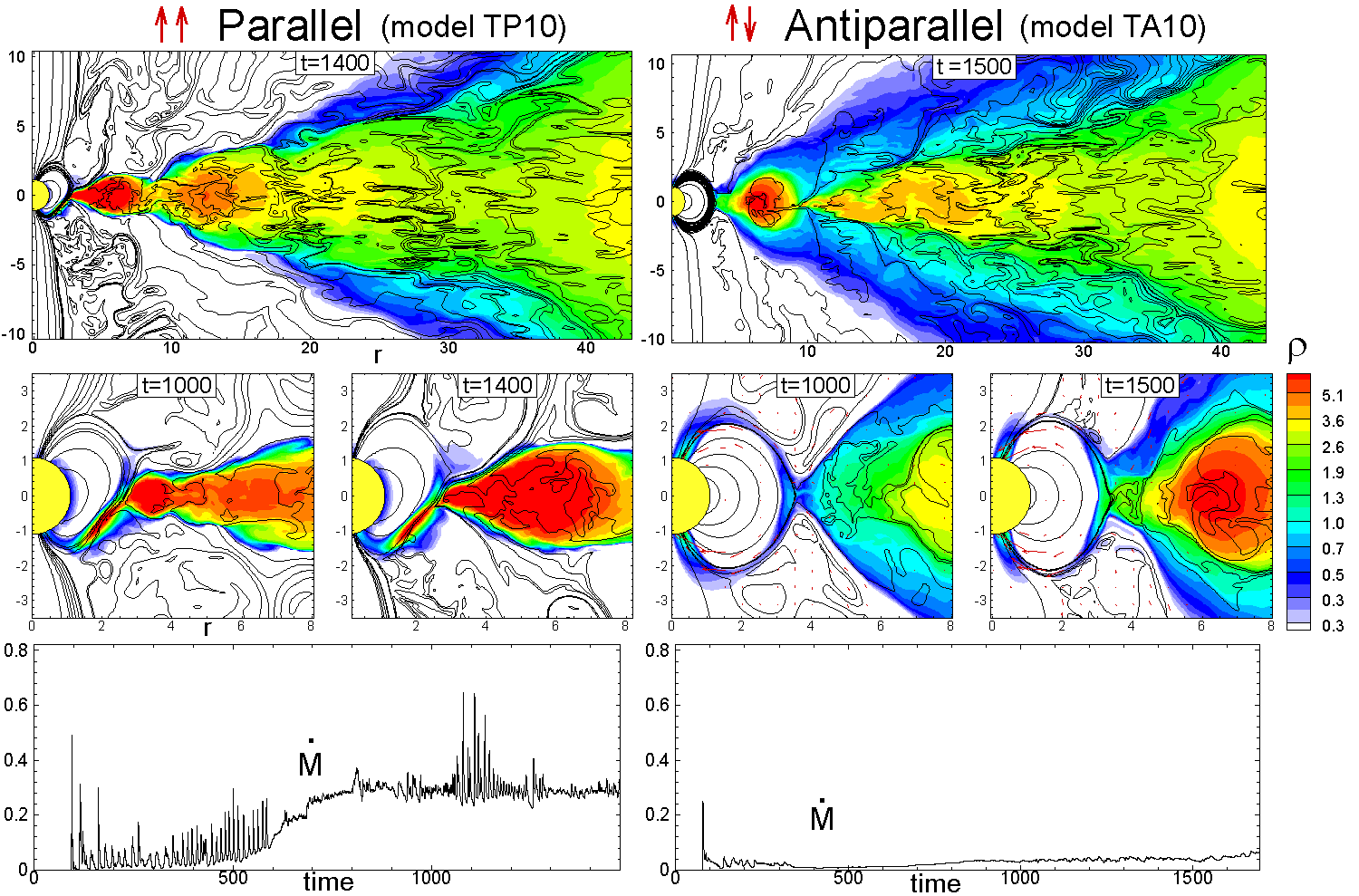
Figure 13: Same as in Fig. 12 but for a medium-sized magnetosphere (models TP10 and TA20).

Figure 14: Same as in Fig. 12 but for models TP5 and TA5 where $\tilde{\mu}=5$. Note the episodic boundary layer accretion observed in model TP5.

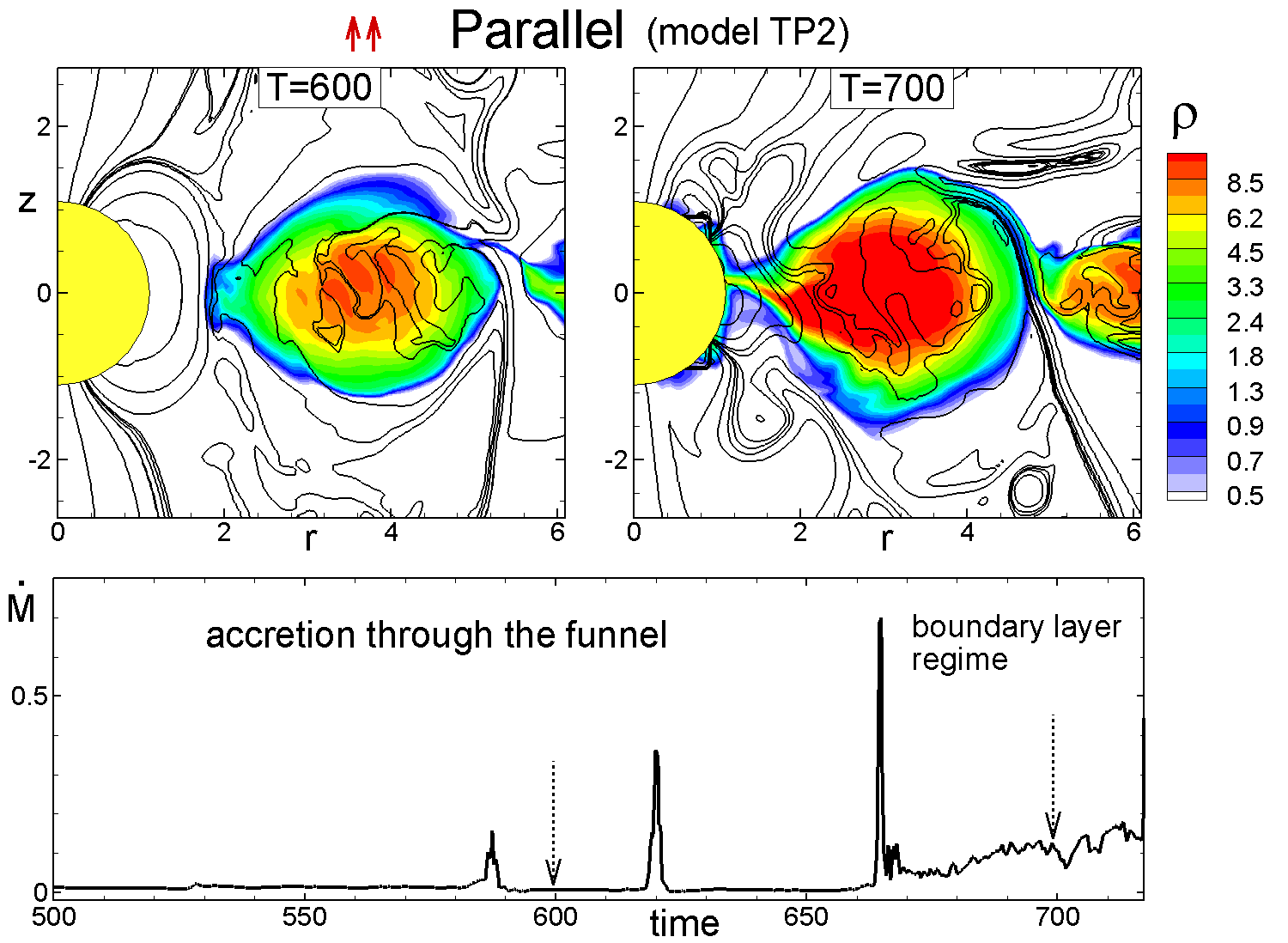
Figure 15: Top panel: Accretion onto a star with a tiny magnetosphere $\tilde{\mu}=2$ and parallel fields (model TP2). Left and right panels show accretion before and after the onset of the boundary layer regime. Bottom panel: Matter flux onto the star shows the transition from the funnel flow accretion (at the left) to the boundary layer regime of accretion (at the right).

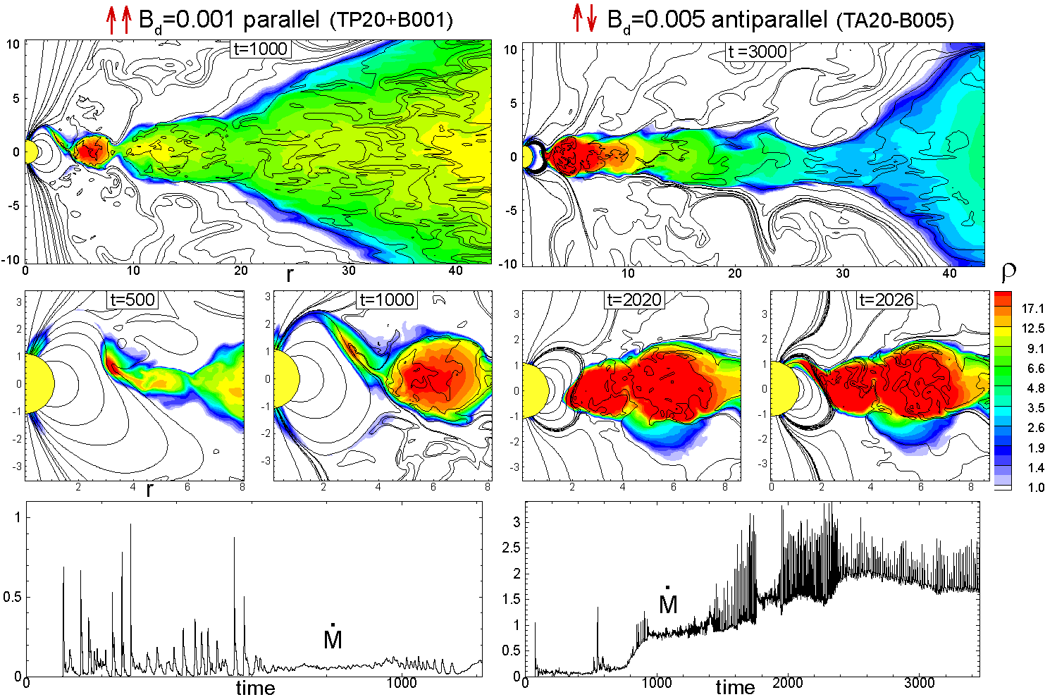
Figure 16: Left panels: Example of accretion and accretion rate in the case of an intermediate-sized magnetosphere and parallel magnetic fields (model TP10). Right panel: Same, but for antiparallel magnetic fields in the disc. We chose moments of time corresponding to bursting and smooth accretion (one per each case).

6 Accretion onto stars with different magnetospheres and accretion rates

Above, we described the case of the largest (in our set of models) magnetosphere, with $\tilde{\mu}=30$. We also calculated accretion onto stars with smaller-sized magnetospheres at magnetospheric parameters $\tilde{\mu}=20,10,5,2$ (see Tab. 1). For homogeneity of results we use the same, tapered topology and the same seed magnetic field in the disc, which can be parallel (sign ‘+’) or antiparallel (sign ‘-’) to the field of the star, and has a $z-$component value $B_{d}=\pm 0.002$.

In two exploratory runs, we fixed the magnetosphere at $\tilde{\mu}=20$, but changed the magnetic field in the disc. In one case, we increased the disc field by a factor of 2.5 and used the antiparallel orientation ($B_{d}=0.005$). In the other case, we decreased the field by half and took the parallel orientation of the field. Below, we analyze results obtained in all these cases.

Fig. 11 shows magnetospheric flow in cases of the different sizes of magnetospheres. For homogeneity, we chose the case of parallel fields, $B_{d}=0.002$ and show data for the moment in time $t=700$. One can see that the size of the magnetosphere decreases with $\tilde{\mu}$, as expected. The funnel stream forms from either top or bottom side of the magnetosphere. In the case of the largest magnetosphere ($\tilde{\mu}=30$), we observed that the funnel formed on one side and stayed there (it moved from the bottom for TP30 and from the top for TA30) during the whole simulation run. In cases of a smaller magnetosphere, the funnel flips between the top and bottom sides, although this happens only a few times per simulation run. The density is usually enhanced at the inner part of the disc, excluding the case of the smallest magnetosphere at $\tilde{\mu}=2$, where the disc accretes directly through the equatorial plane, that is, in the boundary layer regime.

In Sec. 4 we performed an analysis of stresses for models RP30 and TA30 and observed that the accretion rate strongly oscillates in the case of parallel fields, but is much smoother and smaller in the case of antiparallel fields. The question is, how general is this behavior? We realize that initially, the disc is threaded not only with the seed magnetic field, which we introduce at the level of $B_{d}=\pm 0.002$, but also with the magnetic flux of the star, and this flux is larger in cases of larger magnetospheres and can dominate, or can be negligibly small, in cases of smaller magnetospheres. Either way, we expect that the total amount of stress in the disc is different in cases with different $\tilde{\mu}$. Hence, with changing $\tilde{\mu}$, we also change the total amount of stress in the disc. Below we investigate the situation and derive general trends for the value and variability of the accretion rate in different cases.

6.1 Matter flow and accretion rates in different models

First, we show the character of matter flow and accretion rates obtained in different simulation runs. In figures 12,13, and 14, we show results in the same style, where the left and right hand sets of figures correspond to the cases of parallel and antiparallel fields, respectively.

Fig. 12 shows results of simulations for models TP20 and TA20 ($\tilde{\mu}=20$). One can see that the MRI-driven instability has developed in both cases, and in the case of parallel fields matter accretes through episodes of matter accumulation and accretion, and the ‘push’ mechanism of accretion is observed. Simulations show that the accretion rate is high and strongly oscillating (see left bottom panel of Fig. 12). In the right panels we see that in the antiparallel case, the disc is thicker and not as dense. Matter is accumulated near the star in a thick layer, and accretes onto the star, but the accretion rate is lower than in the case of parallel fields, and no oscillations are observed, excluding the first burst discussed in Sec. 5.3

Fig. 13 shows a case with a smaller magnetosphere, $\tilde{\mu}=10$ (models TP10 and TA10). One can see that in cases of parallel fields the disc near the star is thin and the density increases towards the star. Matter accretes through funnel streams. The matter flux at the star has multiple oscillations up to $t\lesssim 600$, then it increases and there are fewer oscillations. We suggest that there are fewer oscillations because the magnetosphere is smaller and it is easier for matter to climb the magnetosphere and form a quasi-steady flow. In the case of antiparallel fields, the density in the disc decreases towards the disc-magnetosphere boundary. The disc is thicker and the accretion rate is lower. We analyze the stresses and discuss possible reasons below.

Fig. 14 shows the case of an even smaller magnetosphere, $\tilde{\mu}=5$ (models TP5 and TA5). One can see that in the case of parallel fields, matter smoothly accretes through the funnel stream, up to time $t\approx 1400$. However, afterwards the accretion becomes bursty, because matter reaches the surface of the star episodically and accretes through the boundary layer (see left bottom panel of Fig. 14). The episodes of accretion are followed by an expansion of the magnetosphere and an accumulation of matter. Then the process repeats, giving multiple bursts observed in the figure. In the case of antiparallel fields (right panels in the figure), the density in the disc decreases towards the star, and the geometry is similar to that observed in model TA10. The accretion rate is quasi-stationary, like in the TA10 case.

Fig. 15 shows an example of a simulation in the case of the smallest magnetosphere considered in our paper, $\tilde{\mu}=2$. The figure shows only the case of parallel fields (model TP2), where we observed the quasi-steady regime of accretion through the boundary layer (top right panel). In the case of antiparallel fields, accretion is similar to that in model TA5, but the magnetosphere is somewhat smaller. Interestingly, when the disc accretes through the boundary layer, the magnetic field of the star is compressed by the disc and obtains a complex geometry.

There are a few factors which determine the differences in matter flow and accretion rates seen in different models:

• Different orientation of the disc field relative to the stellar field (parallel and antiparallel cases) leads to different magnetic topologies at the boundary and can influence matter flow at the disc-magnetosphere boundary;

• In cases of same/opposite orientations of the field, the magnetic stress is higher/lower at the boundary;

• In cases with lager/smaller $\tilde{\mu}$, the stellar magnetic field contributes more/less to the total magnetic energy of the disc, so that the accretion rate is different.

Often, these factors act simultaneously, and it is difficult to separate one from another. To investigate the dependence of processes on the accretion rate, we chose the magnetosphere with $\tilde{\mu}=20$, and performed two additional runs. In one of them, we increased the field in the disc by a factor of 2.5: $B_{d}=-0.005$. In the case of parallel fields, we expected a higher accretion rate and bursty accretion. This is why we chose antiparallel fields, where the situation is less clear (the model TA20-005). In another test case, we decreased the field by a factor of two: $B_{d}=0.001$. We know that in the case of antiparallel fields we would again observe a very low accretion rate. Thus, we chose the case of parallel fields, where the lower accretion rate could yield a different result (model TP20+001).

Fig. 16 shows these two cases where the left and right panels correspond to these test models. We observed that for $B_{d}=0.001$ (left panels), the accretion rate in the disc is lower compared with the base case (TP20) and the density in the inner parts of the disc is lower as well. We observed that accretion is bursty during about 600 rotations, but later a steady funnel stream is formed. The accretion rate onto a star is a few times lower compared with the TP20 case. Comparison of these two cases shows that for the persistent bursty accretion (observed in TP20), one needs higher accretion rate, at which the magnetosphere is bent and traps the accreting matter. Hence, the parallel field configuration is favorable for matter trapping and bursty accretion, but it is not the only condition.

Fig. 16 (right panels) shows that a stronger magnetic field in the disc generates stronger MRI-driven turbulence, and the accretion rate is much higher than in any of the above models. We observed that in such a situation, the inner disc bends the magnetosphere; the ‘push’ mechanism is switched on and we observe the persistent bursty accretion. This is not typical for the case of antiparallel fields in above models. We conclude that the bursty accretion can appear in the cases of both parallel and antiparallel fields if the accretion rate is high. We should note, however, that this is a special case where the accretion rate is very high, so that the initial rapid accretion strongly reconstructs the disc.

In all above cases, we have different initial magnetic flux in the disc. To compare the total magnetic energy stored in the disc, we separated the disc using the density level $\rho=0.3$, integrated stresses and pressure in the whole disc, and calculated these values per unit volume. Fig. 17 shows values $\bar{\alpha_{f}}={2/3}\langle{T_{f}}\rangle/\langle{P_{m}}\rangle$ and $\bar{\beta}=\langle{P_{m}}\rangle/\langle{P_{f}}\rangle$. The right panel of the figure shows that the value of $\bar{\beta}$ is very high in the beginning, but drops rapidly because the $B_{\phi}-$field strongly increases. So, at $t=1000$, $\bar{\beta}$ varies between 3 and 6 for our main models, and is about 1 and 12 for test models. These numbers are reasonable for the MRI accretion discs (e.g., Hawley 2000). The volume-averaged parameter $\bar{\alpha}$ (at $t=1000$) varies in the range of $0.01-0.016$ for the main models, and is smaller ($0.006$) and larger ($0.035$) for test models. We should note that apart from the model TP30, all other models have quite similar averaged parameters in the disc, so that the accretion disc properties are not that different in different cases. Therefore, we can use different runs for analysis of other characteristics of the disc-magnetosphere boundary, such as dependence on reconnection and the local stress depression due to different orientations of the field. The test cases are different from the main models, but this was the goal - to check the difference, and we consider and analyze these cases separately. Note that the volume-averaged stresses and $\alpha_{f}-$parameters are about twice as small compared with those at the disc-magnetosphere boundary (see next section).

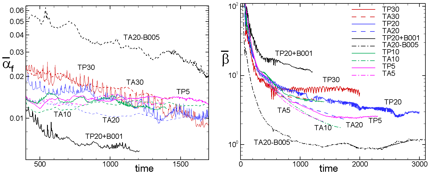
Figure 17: Left Panel: The magnetic parameter $\alpha_{f}$ is averaged along the volume of the disc, $\bar{\alpha_{f}}$, and is shown as a function of time. Only part of the simulation time is shown for clarity of results. Right Panel: Volume averaged plasma parameter $\bar{\beta}$ as a function of time.

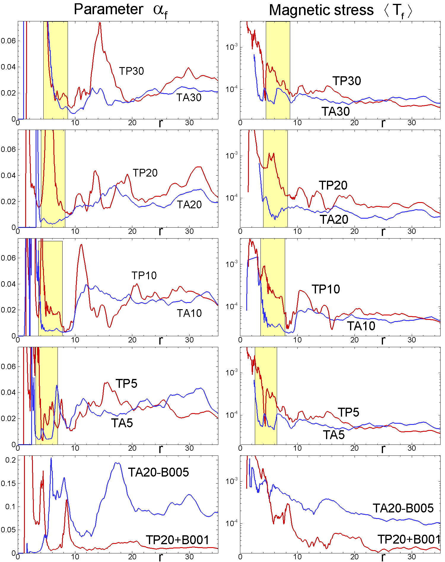
Figure 18: Left panels: Radial distribution of the magnetic diffusivity parameter $\alpha_{f}$ in the equatorial plane at sample time $t=1000$ for models with different magnetospheric sizes (parameters $\tilde{\mu}$). Right panels: same but for magnetic stresses. The bottom row shows test cases with 2.5 times larger (model TA20-005) and 2 times smaller (model TP20+001) values of the magnetic field in the disc, compared with the base field of $B_{d}=0.002$.

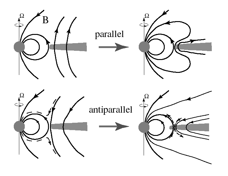
Figure 19: Top panels: Sketch of the disc-magnetosphere interaction in case of parallel fields (where the disc magnetic field has the same direction as the stellar field). In this case, the magnetic flux of the same polarity is accumulated at the boundary, and the magnetosphere is bent by the disc in the equatorial plane. Bottom panels: Same but for antiparallel fields. The dashed curve in the left panel shows the suggested field topology after reconnection. The dashed lines in the right panel show the $X-type$ reconnection point.

6.2 Analysis of cases of parallel and antiparallel fields

Here we perform an additional analysis of all cases with the aim of understanding the role of the field orientation (parallel versus antiparallel) in different cases.

Sketches in Fig. 19 show the expected topologies of the field at the disc-magnetosphere boundary in cases of parallel and antiparallel fields. The top panel shows that in the case of unidirectional (parallel) fields of the disc and the star, magnetic flux of the same polarity is accumulated at the boundary and traps the matter. We suggest that this might be a factor which leads to oscillating accretion. Our simulations of the main models ($B_{d}=\pm 0.002$) show that accretion rate varies from case to case, but we observe bursty accretion in the case of parallel fields. The test cases in models TA20-005 and TP20+0.001 show that the orientation of the field is not the only reason for bursty accretion. Nevertheless, we clearly see the tendency for parallel fields to favor bursty accretion.

The right panel in Fig. 19 shows how the topology of the field at the magnetosphere boundary changes as the result of reconnection. It is interesting to note that reconnection between the field of the star and oppositely oriented field of the disc leads to the field lines which begin at the star but then stretch out towards the disc, and often go along the disc. Hence, the reconnection lets matter flow towards the deeper field lines of the closed magnetosphere, and therefore acts as an efficient diffusivity. On the other hand, the distribution of the field lines after reconnection has a tendency to block formation of the funnel flow towards the star. We suggest that this factor can be important in both decreasing the accretion rate and making accretion smoother. The test model TA20-B005 shows a different evolution, but this is a somewhat special case. We think that the opposite polarity of the fields is not a sufficient condition for smooth accretion. However, at moderate accretion rates, we would expect less bursty accretion than in the case of parallel fields.

Note that the situation is analogous to the Solar wind interaction with the Earth’s magnetosphere, where one orientation of the solar wind B-field allows for reconnection and the other one does not (e.g., Frey et al 2003).

Another important issue is that the magnetic stress at the disc-magnetosphere boundary is larger/smaller in cases of parallel/antiparallel fields. This can lead to a local decrease in the accretion rate at the boundary. We integrated stresses in the $z-$direction, and plotted them as a function of radius at $t=1000$. Fig. 18 (right panels) shows the radial distribution of magnetic stresses $\angle{T_{f}}\rangle$, where red and blue lines indicate parallel and antiparallel fields, respectively. One can see that at the inner boundary, stresses are systematically (about 10 times) larger in cases of parallel fields. The region where stresses are different is located to the right of the magnetically-dominated magnetosphere, and has a typical thickness of $\Delta r_{\rm stress}=4R_{0}$. The size of the magnetosphere decreases with $\tilde{\mu}$ and hence this region of different stresses (see yellow-color region in Fig. 18) moves slightly to the left. The left panel shows that the $\alpha-$parameter is also systematically larger in cases of parallel fields, although the result is not as clean because matter pressure $\langle{P_{m}}\rangle$ varies and is in the denominator of $\alpha_{f}$. For example, $\langle{P_{m}}\rangle$ is higher in cases of parallel fields. Nevertheless, we see enhancements of $\alpha$ in models with $\tilde{\mu}=20,10,5$. We conclude that the orientation of the field does change the local accretion rate in the region of the inner disc that is adjacent to the magnetosphere.

Fig. 18 also gives a representative number for $\alpha_{f}$ in different models. One can see that this parameter varies in the range of $\alpha_{f}\approx 0.01-0.04$ with an average value of $\alpha_{f}\approx 0.02-0.03$ for all our standard models. Note that at $r\gtrsim 10$, discs with parallel and antiparallel fields give similar $\alpha_{f}$.

The bottom plots of Fig. 18 show our test cases. One can see that for $B_{d}=-0.005$, the stress is much larger and $\alpha_{f}\approx 0.1$ on average, while for $B_{d}=0.001$, the stress is smaller than in our main cases, and $\alpha_{f}\approx 0.01-0.02$.

7 Magnetically-dominated corona

Initially, we have a low-density corona threaded by the dipole magnetic field. The differential rotation of the foot-points of loops (threading the disc and the star) could lead to the inflation of the field lines and to the expansion of the corona (Lovelace et al., 1995). Both, the coronal expansion and the MRI instability occur with the same time-scale of Keplerian rotation at a given radius $r$. However, we observed that the global inflation of the coronal magnetosphere has been strongly disturbed by the initial penetration of the inner disc through the external magnetosphere. We observed that the initial penetration led to a strong reconnection event (see Fig. 10) and a large magnetic island formed and moved outward along the disc. This island pushed the coronal field lines threading the disc to larger radii. Subsequent events of reconnection led to the formation of many more (but smaller) islands, which formed the turbulent component of the magnetically-dominated corona. The field lines connecting a star with the external corona inflated and formed an elongated field structure propagating up and down. Subsequent evolution led to the winding of the coronal field lines and to the formation of a magnetically-dominated corona with a high azimuthal component of the field. The corona expanded slowly to larger and larger distances from the disc. We investigated the corona using one of our typical cases (model TP20). Simulations show that the magnetically-dominated corona reached the top and bottom boundaries of the region at $t\approx 3000P_{0}$, which corresponds to about 30 rotations at the grid center (in the $r-$direction). The inner parts of the corona, closer to the star, are turbulent and represent multiple magnetic islands. The external 2/3 of the disc are threaded with the ordered magnetic field expanding outward. Interestingly, no disc wind flows from the disc to the corona along these lines, in spite of the high inclination of these field lines towards the disc. In addition, the magnetic field is tightly wrapped in the corona and a high gradient of magnetic pressure is observed. In spite of that, neither centrifugally-driven, nor magnetically-driven wind was formed along these field lines. This issue requires further investigation.

This magnetic, slowly moving corona resembles the corona formed in Miller & Stone (2000) simulations. However, in their simulations, the field in the corona has been generated in the disc and moved upward as a result of buoyancy. In our simulations, the field originates from the initial coronal field of the star, but is strongly wrapped by the rotation of the disc.

Fig. 20 shows different features of the corona. The left panel shows that the corona has low density. Next panel (to the right) shows that the expanding region of the corona is magnetically-dominated (plasma parameter $\beta<<1$). The next plot shows that the corona rotates approximately with an angular velocity of the disc. Next plot shows that the azimuthal field $B_{\phi}$ is strong and that there is an outwardly directed gradient of magnetic pressure. The azimuthal field is about 10-100 times stronger than the poloidal field. The right panel shows that matter in the expanding corona is cold and hence the corona expands due to magnetic pressure.

This new type of magnetic structure is not a jet but instead a magnetic formation filled with the ordered (mainly azimuthal) and turbulent magnetic field which slowly expands in the axal direction.

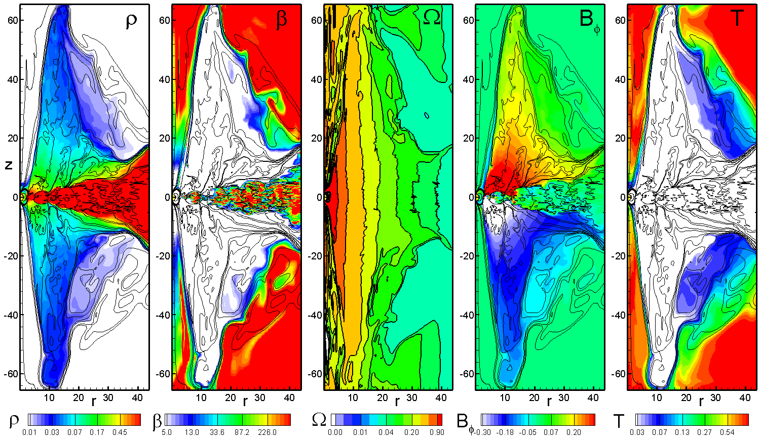
Figure 20: Distribution of different values in the whole simulation region in the model TP20 at time $T=3000$. The lines are sample magnetic field lines. The color background (from left to right): density ($\rho$), $\beta-$parameter, angular velocity ($\Omega$), azimuthal magnetic field ($B_{\phi}$), and temperature ($T$).

8 Astrophysical examples

Table 2 shows typical reference values. Below are a few examples where the values obtained in simulations are converted to dimensional values for typical CTTSs, magnetic CVs and millisecond pulsars.

8.1 Application to Classical T Tauri stars

We consider a few simulation runs relevant to $\tilde{\mu}=20$ (TP20, TA20, etc.) and convert dimensionless numbers presented in the paper to dimensional values.

The reference values shown in Tab. 2 are relevant to stars with different $\tilde{\mu}$, but the magnetic field of the star $B_{\star}$ is different for different $\tilde{\mu}$. For $\tilde{\mu}=20$, we obtain an equatorial field: $B_{\star}^{eq}=\tilde{\mu}B_{0}=1000$G (and polar field $B_{\star}^{p}=\tilde{\mu}*B_{0}=2000$G). The $z-$component of the seed magnetic field in the disc is $B_{d}=0.002B_{0}=0.1$G, and the azimuthal component of the field amplifies up to $B_{\phi}\approx 0.5-1$G. The magnetic field of the star at the disc-magnetosphere boundary (say, at $3R_{\star}$) is $B=37$G, that is, much larger than the field in the disc. Fig. 12 (bottom panels) shows accretion rate $\widetilde{\dot{M}}$ in cases of parallel and antiparallel fields. In the case of parallel fields we see that the accretion rate varies in the range $\widetilde{\dot{M}}\approx 0.1-0.8$ with bursts up to $1.5$, which corresponds to dimensional values ${\dot{M}}_{parallel}=\widetilde{\dot{M}}M_{0}\approx(0.6-3.6)\times 10^{-8}\rm{M}_{\odot}\rm{yr}^{-1}$ with bursts up to $8.4\times 10^{-8}\rm{M}_{\odot}\rm{yr}^{-1}$. In model TA20 (with antiparallel fields), the accretion rate is much smaller, $\widetilde{\dot{M}}=0.01-0.05$, and the dimensional accretion rate is ${\dot{M}}_{antiparallel}=\widetilde{\dot{M}}M_{0}\approx(0.1-2.8)\times 10^{-9}\rm{M}_{\odot}\rm{yr}^{-1}$. Hence, if the global magnetic field alternates polarities, then the accretion rate may vary from higher values and oscillating character to lower rates with no oscillations. The time-scale between oscillations is $\Delta t\times P_{0}=0.37{\rm days}\times 35=13$ days, and about half of this value for later times. Note that values of accretion rate will increase if we take a larger magnetic field of the star and hence larger $B_{0}$. The dependence is $\dot{M}\sim B_{\star}^{2}$.

8.2 Application to millisecond pulsars

For $\tilde{\mu}=20$, we obtain the equatorial field of the star $B_{\star}^{eq}=\tilde{\mu}B_{0}=10^{9}$G and the polar field $B_{\star}^{p}=2\times 10^{9}$ G. The $z-$component of the seed magnetic field in the disc, $B_{d}=0.002B_{0}=10^{6}$G, and the azimuthal component of the field amplifies up to $B_{\phi}\approx 10^{7}$G. Fig. 12 (bottom panels) shows accretion rate $\widetilde{\dot{M}}$ in cases of parallel and antiparallel fields. In the case of parallel fields the accretion rate varies in the range $\widetilde{\dot{M}}\approx 0.1-0.8$, with bursts up to $1.5$, which corresponds to dimensional values ${\dot{M}}_{parallel}=\widetilde{\dot{M}}M_{0}\approx(0.23-1.8)\times 10^{-8}\rm{M}_{\odot}\rm{yr}^{-1}$, with bursts up to $3.4\times 10^{-8}\rm{M}_{\odot}\rm{yr}^{-1}$. In model TA20 (with antiparallel fields), the accretion rate is much smaller, $\widetilde{\dot{M}}=0.01-0.05$, and the dimensional accretion rate is ${\dot{M}}_{antiparallel}=\widetilde{\dot{M}}M_{0}\approx(0.23-1)\times 10^{-9}\rm{M}_{\odot}\rm{yr}^{-1}$. Hence, if the global magnetic field alternates polarities, then the accretion rate may vary from higher values and oscillating character to lower rates with no oscillations. The time scale between oscillations is $\Delta t\times P_{0}=0.46{\rm ms}\times 35=16$ ms, and about half of this value for later times. Note that the interval between bursts increases with the spin of the star and reaches the value of $300$ in the propeller regime (Ustyugova et al., 2011). This gives a much longer interval between bursts, $\Delta t_{bursts}=138$ ms. In a real astrophysical situation, where the diffusivity is probably even smaller than in our simulations, one can expect even longer intervals between bursts. Some millisecond pulsars show accretion in a flaring regime. For example, the pulsar SAX J1808.4-3658 shows flaring activity in the tail of the burst with a quasi-period of 1Hz (Patruno et al., 2009). We suggest that these flares may be connected with the disc-magnetosphere interaction in the propeller regime (see also Romanova et al. 2004, 2005; Ustyugova et al. 2006; Romanova et al. 2009).

9 Conclusions

We performed axisymmetric simulations of accretion onto magnetized stars from MRI-driven discs. The main conclusions are the following:

• Long-lasting, MRI-driven accretion has been developed in the disc where the magnetic stresses determine the accretion rate with equivalent parameter $\alpha_{m}\approx 0.02-0.04$ (with larger and smaller values in test models).

• We observed that the matter-dominated turbulent disc is stopped by the dipole field of the star at the radius where the magnetic stress of the magnetosphere matches the matter stress in the disc. Matter is lifted above the magnetosphere and flows in funnel stream, which usually picks one of the sides (top or bottom), and may switch sides a few times during the simulation run.

• Processes at the disc-magnetosphere boundary depend on the orientation of the poloidal field in the disc:

  (1). Parallel fields: If the field has the same direction as the stellar field at the boundary, then the magnetic stress and accretion rate are locally enhanced. However, the field of same polarity is accumulated at the boundary and matter is trapped. This matter bends the field lines of the magnetosphere near the equator, and accretion is prohibited. Later, matter is accumulated and flows to the star through a temporary funnel stream, and the magnetosphere expands again. Then the process repeats. This leads to strong oscillations of the accretion flux on the star. Such oscillations appear as the result of a relatively high accretion rate, as determined by MRI, and low diffusivity at the disc-magnetosphere boundary. In a test run with lower accretion rate ($\alpha_{m}\approx 0.01$), temporary oscillations were followed by quasi-stationary accretion through the funnel flow.

  (2).  Antiparallel fields: If the fields of the star and the disc have opposite directions, then reconnection of the field at the disc-magnetosphere boundary can help matter penetrate towards deeper layers of the closed magnetosphere. At the same time, the magnetic flux cancellation lowers the magnetic stress locally, within a few stellar radii of the magnetosphere. This leads to lower accretion rate. In addition, the magnetic configuration of the stellar field after reconnection is not favorable for formation of the funnel stream. Both factors lead to quasi-steady accretion through a weak funnel stream, and to lower accretion rates compared with the case of parallel fields. In the test run with much higher accretion rate ($\alpha_{m}\approx 0.1$), the effect of stress diminishing and other factors becomes unimportant, and matter accretes in bursty regime like in case (1).

• MRI-driven turbulence provides outward angular transport and inward flow of matter, and gives a significant viscosity. However, it does not give magnetic diffusivity at the disc-magnetosphere boundary. We often have a situation where the Prandtl number is high, $Pr_{m}=\nu_{vis}/\nu_{dif}>>1$, at the disc-magnetosphere boundary. In many cases, reconnection helps matter penetrate towards deeper layers of the magnetosphere and acts as an efficient diffusivity. In other cases, small, but finite numerical diffusivity helps.

• We point out the importance of the initial interaction of the disc with the magnetosphere, where the disc comes from some distance after a period of low accretion. Such a situation is expected in many astrophysical systems where a star has a dynamically-important magnetic field. Then the inner disc compresses the star’s magnetic flux and moves towards the star. Matter, after accumulation, flows towards the star and pushes this magnetic flux to reconnect. This leads to a strong burst in the accretion rate. This may also lead to a strong X-ray flare resulting from the reconnection of the magnetic field.

• A magnetically-dominated corona forms above and below the disc and slowly expands in the axial direction. The magnetic field is tightly wrapped and the azimuthal field is 10-100 times stronger than the poloidal field. The corona is cold and it expands due to the magnetic pressure gradient.

The simulations presented here are restricted to axisymmetric conditions. Earlier comparisons of axisymmetric and 3D simulations of MRI-driven accretion discs show good similarity (Hawley, 2000), and we suggest that our disc is sufficient for investigation of the disc-magnetosphere interaction. However, the main restriction is probably in the fact that in the full 3D approach matter can penetrate the magnetic field due to the Raleigh-Taylor instability (Arons & Lea, 1976). Global 3D simulations show that for some conditions, the disc matter can penetrate the magnetosphere of the star, in particular in cases of small tilts of the dipole field and slowly rotating stars (Romanova et al. 2005; Kulkarni & Romanova 2008). Hence, it is important to investigate the MRI-driven accretion onto magnetized stars in full 3D approach. We discuss results of global 3D simulations in Romanova et al. (2011).

The described research may have multiple applications to different astrophysical objects. Many X-ray binaries show accretion in a flaring regime. For example, the pulsar SAX J1808.4-3658 shows flaring activity in the tail of the burst with a quasi-period of 1Hz (Patruno et al., 2009). We suggest that these flares may be connected with the process of matter accumulation at the disc-magnetosphere boundary with subsequent accretion, similar to that observed in our case of parallel fields (see Fig. 9). In this case the unidirectional magnetic flux blocks the accretion. This effect is similar to the propeller effect, where the centrifugal barrier blocks the accretion, and accretion occurs episodically (e.g., Romanova et al. 2004, 2005; Ustyugova et al. 2006; Romanova et al. 2009; see also Spruit & Taam (1990, 1993) and D’Angelo & Spruit (2010)). In this paper we considered only slowly rotating stars. Preliminary axisymmetric simulations of accretion in the propeller regime from MRI-driven discs show that the interval between accretion events strongly increases with the spin of the star (Ustyugova et al., 2011).

Appendix A Code description, initial and boundary conditions and reference units

A.1 Basic Equations

The matter flow is described by the equations of ideal MHD:

$${\frac{\partial\rho}{\partial t}+{\bf\nabla}\cdot\left(\rho{\bf v}\right)}=0~{},$$ (11)

$${\frac{\partial(\rho{\bf v})}{\partial t}+{\bf\nabla}\cdot{\cal T}}=\rho~{}{\bf g}~{},$$ (12)

$$\frac{\partial{\bf B}}{\partial t}-{\bf\nabla}\times({\bf v}\times{\bf B})=0~{},$$ (13)

$${\frac{\partial(\rho S)}{\partial t}+{\bf\nabla}\cdot(\rho S{\bf v})}=0~{}.\$$ (14)

Here, $\rho$ is the density and $S$ is the specific entropy; $\bf v$ is the flow velocity; $\bf B$ is the magnetic field; $\cal{T}$ is the momentum flux-density tensor; and ${\bf g}$ is the gravitational acceleration due to the star, which has mass $M$. The total mass of the disc is negligible compared to $M$. The plasma is considered to be an ideal gas with adiabatic index $\gamma=5/3$, and $S=\ln(p/\rho^{\gamma})$. We use cylindrical coordinates $(r,z,\phi)$. The condition for axisymmetry is $\partial/\partial\phi=0$.

A.2 Reference Units

The MHD equations are solved using dimensionless variables $\widetilde{A}$. To obtain the physical dimensional values $A$, the dimensionless values $\widetilde{A}$ should be multiplied by the corresponding reference units $A_{0}$; $A=\widetilde{A}A_{0}$. To choose the reference units, we first choose the stellar mass $M_{\star}$ and radius $R_{\star}$. The reference units are then chosen as follows: mass $M_{0}=M_{\star}$, distance $R_{0}=R_{\star}$, velocity $v_{0}=(GM_{0}/R_{0})^{1/2}$, time scale $P_{0}=2\pi R_{0}/v_{0}$, angular velocity $\Omega_{0}=v_{0}/R_{0}$. The equatorial magnetic field is determined as $B_{\star}=\tilde{\mu}B_{0}$ where $B_{0}$ is the reference magnetic field at $R_{0}$. The parameter $\tilde{\mu}$ is used to vary the magnetic field of the star. We chose $B_{0}$ such a way, that for $\tilde{\mu}=10$, we have a field typical for a given type of stars. For example, for CTTS, the choice of $B_{0}=50$G, gives equatorial field $B_{\star}=\tilde{\mu}=500$G (and polar field $1000$G) which is typical for CTTSs. Then the models with larger/smaller values of $\tilde{\mu}$, correspond to smaller/larger magnetic field of the star. We then define the reference dipole moment $\mu_{0}=B_{0}R_{0}^{3}$, density $\rho_{0}=B_{0}^{2}/v_{0}^{2}$, pressure $p_{0}=\rho_{0}v_{0}^{2}$, mass accretion rate $\dot{M}_{0}=\rho_{0}v_{0}R_{0}^{2}$, the torque $N_{0}=\rho_{0}v_{0}^{2}R_{0}^{3}$. energy per unit time $\dot{E}_{0}=\rho_{0}v_{0}^{3}R_{0}^{2}$. Temperature $T_{0}=\mathcal{R}p_{0}/\rho_{0}$, where $\mathcal{R}$ is the gas constant. , and the effective blackbody temperature

Therefore, the dimensionless variables are $\widetilde{r}=r/R_{0}$, $\widetilde{v}=v/v_{0}$, $\widetilde{t}=t/P_{0}$, $\widetilde{B}=B/B_{0}$, $\widetilde{\mu}=\mu/\mu_{0}$ and so on. In the subsequent sections, we show dimensionless values for all quantities and drop the tildes ($\sim$). Our dimensionless simulations are applicable to different astrophysical objects with different scales. We list the reference values for typical CTTSs, cataclysmic variables, and millisecond pulsars in Tab. 2.

	CTTSs	White dwarfs	Neutron stars
$M_{\star}(M_{\odot})$	0.8	1	1.4
$R_{\star}$	$2R_{\odot}$	5000 km	10 km
$B_{1\star}$ (G)	$5\times 10^{2}$	$5\times 10^{5}$	$5\times 10^{8}$
$R_{0}$ (cm)	$1.4\times 10^{11}$	$1.4\times 10^{9}$	$2.9\times 10^{6}$
$v_{0}$ (cm s-1)	$2.8\times 10^{7}$	$5.2\times 10^{8}$	$1.4\times 10^{10}$
$\Omega_{0}$ (s-1)	$2\times 10^{-4}$	1.03	$1.4\times 10^{4}$
$P_{0}$	$0.37$ days	6.1 s	0.46 ms
$B_{0}$ (G)	50	$5.0\times 10^{4}$	$5\times 10^{7}$
$\rho_{0}$ (g cm-3)	$3.3\times 10^{-12}$	$3.7\times 10^{-8}$	$5.3\times 10^{-5}$
$p_{0}$ (dy cm-2)	$2.5\times 10^{3}$	$1.0\times 10^{10}$	$1.0\times 10^{16}$
$\dot{M}_{0}(M_{\odot}$yr${}^{-1})$	$5.6\times 10^{-8}$	$1.5\times 10^{-7}$	$2.3\times 10^{-8}$
$N_{0}$ (g cm2s-2)	$6.9\times 10^{36}$	$1.2\times 10^{36}$	$1.0\times 10^{34}$
$\dot{E}_{0}$ (erg s-1)	$1.3\times 10^{33}$	$1.3\times 10^{36}$	$1.4\times 10^{38}$

Table 2: Sample reference units for typical CTTSs, white dwarfs, and neutron stars. The field $B_{\star}$ corresponds to the case $\tilde{\mu}=10$. Real dimensional values for variables can be obtained by multiplying the dimensionless values of variables by these reference units.

A.3 Code description

We solve the full set of axisymmetric ideal MHD equations in cylindrical coordinates using the Godunov-type numerical method. To solve the set of ideal MHD equations, we use an approximate multi-state HLL Riemann solver similar to one described recently by Miyoshi & Kusano (2005). Compared with Miyoshi & Kusano (2005), we solve an equation for the entropy instead of full energy equation. This approximation is valid in cases where shocks are not important, like in our case. In Miyoshi & Kusano (2005), the procedure of the calculations of the MHD equations is described in detail. Here, we briefly summarize the main features of our method: the MHD-variables are calculated in four states bounded by five MHD discontinuities: the contact discontinuity, two Alfven waves and two fast magnetosponic waves. Compared with Miyoshi & Kusano (2005), we performed the procedure of correction for the fast magnetosonic waves velocity so that to support the gap between these waves and the Alfvén waves which propagate behind the fast magnetosonic waves. This helps us to escape the “non-physical” solutions of the Riemann problem. To satisfy the condition of the zero divergency of the magnetic field, we introduced the $\phi-$component of the magnetic field potential which has been calculated using the method proposed by Gardiner & Stone (2005). To decrease the error in the approximation of the Lorentz force, we use the splitting of the field to the dipole and calculated components, $B=B_{dip}+B^{\prime}$, and dropped terms of the order of $B_{dip}^{2}$ which give zero input into the Maxwellian stress tensor (Tanaka, 1994). No viscosity or diffusivity has been added to the code, and hence we investigated accretion driven only by the MRI-turbulence. Our code has been extensively tested (see tests and other details in Koldoba et al. 2011).

A.4 Initial conditions

The initial conditions are similar to those used in Romanova et al. (2005) and Ustyugova et al. (2006). Here, we summarize these conditions.

The disc is cold with temperature $T_{d}$ and dense with density $\rho_{d}$, while the corona is hot $T_{c}=1000T_{d}$ and rarefied $\rho_{c}=0.001\rho_{d}$. We place both the disc and the corona into the simulation region. We assume that the initial flow is barotropic with $\rho=\rho(p)$, and that there is no pressure jump at the boundary between the disc and corona. Then the initial density distribution (in dimensionless units) is the following:

$$\rho(p)=\left\{\begin{array}[]{lcl}p/{\cal R}T_{d}~{},~{}~{}~{}p>p_{b}~{}~{}~{}~{}{\rm and}~{}~{}~{}~{}r\geq r_{b}~{},\\[8.5359pt] p/{\cal R}T_{c}~{},~{}~{}~{}~{}p<p_{b}~{}~{}~{}~{}{\rm or}~{}~{}~{}~{}~{}~{}r\leq r_{b}~{},\end{array}\right.$$

where $p_{b}$ is the pressure on the surface which separates the cold matter of the disc from the hot matter of the corona. On this surface the density jumps from $p_{b}/T_{d}$ to $p_{b}/T_{c}$. Here $r_{b}$ is the inner disc radius. Because the density distribution is barotropic, the angular velocity is constant on coaxial cylindrical surfaces about the $z-$axis. Consequently, the pressure distribution may be determined from the Bernoulli equation,

$$F(p)+\Phi+\Phi_{c}=E={\rm const}~{}.$$

Here, $\Phi=-GM/|{\bf r}|$ is gravitational potential, $\Phi_{c}=\int_{r\sin\theta}^{\infty}\Omega^{2}(\xi)\xi d\xi$ is centrifugal potential, which depends only on the cylindrical radius $r\sin\theta$, and

$$F(p)=\left\{\begin{array}[]{lcl}{\cal R}T_{d}\ln(p/p_{b})~{},~{}~{}~{}p>p_{b}~{}~{}~{}~{}{\rm and}~{}~{}~{}r\sin\theta>r_{b}~{},\\[8.5359pt] {\cal R}T_{c}\ln(p/p_{b})~{},~{}~{}~{}~{}p<p_{b}~{}~{}~{}~{}{\rm or}~{}~{}~{}~{}r\sin\theta<r_{b}~{}.\end{array}\right.$$

The angular velocity of the disc is slightly super-Keplerian, $\Omega(z=0)=\kappa\Omega_{K}$ ($\kappa=1+0.02$), due to which the density and pressure increase towards the periphery. Inside the cylinder $r\leq r_{b}$ the matter rotates rigidly with angular velocity of the star $\Omega(r_{b})=\kappa(GM/r_{b}^{3})^{1/2}$. We place the inner edge of the disc at $r_{b}=10$ and rotate a star with angular velocity $\Omega(r_{b})=10^{-3/2}\approx 0.03$. The disc evolves, but we keep a star rotating slowly to be sure that it represents the gravitational well for the incoming matter (see the case of rapidly rotating stars in Ustyugova et al. 2011).

Initially, the region is threaded with the dipole magnetic field of the star. We use different values of the magnetospheric parameter $\tilde{\mu}$ from 30 to 2 (see Tab. 1). This parameter is responsible for the size of the magnetosphere in dimensionless runs. in the disc. The initial density in the disc varies from $\rho_{d}=1$ (at the inner edge) up to $\rho_{d}=4.6$ (at the outer boundary).

A.5 Boundary Conditions

On the star: The dipole magnetic field is frozen into the surface of the star, that is the normal to the surface component of the field is fixed, while azimuthal component has “free” boundary condition, $\partial{B_{\phi}}/\partial n=0$. There is also free boundary conditions for all other variables A, $\partial A/\partial n=0$. Additional condition is applied to the poloidal velocity which forbids matter to flow out of the star. In addition, in the last grid we adjust the total velocity vector to be parallel to the total magnetic field vector. This helps to strengthen the frozen-in condition near the star and to enhance the divergency-free condition at the boundary.  The top and bottom boundaries: The values of density $\rho$, entropy $s$ and azimuthal field $B_{\phi}$ are fixed. Free conditions for all other variables ($B_{r}$, $B_{z}$, $v_{r}$, $v_{z}$, $v_{\phi}$). In addition, $v_{z}=0$ in case if matter flows into the simulation region.  The side boundary: The side boundary is divided into the “the disc region” at $|z|<z_{d}$ and “corona region” at $|z|>z_{d}$, where

$$z_{d}=\sqrt{\bigg{[}\frac{GM}{F_{c}(R_{out})}\bigg{]}^{2}-R_{out}^{2}},$$

where $F_{c}(R_{out})=aGM/R_{out}$ is centrifugal potential and $R_{out}$ is the external radius. In the disc ($|z|<z_{d}$) we have an inflow condition for the matter. Namely, we push matter into the region with small velocity:

$$v_{r}=-\delta\frac{3}{2}\frac{p}{\rho v_{K}(R_{out})},~{}~{}\delta=0.02,$$

and with poloidal magnetic field corresponding to the initial magnetic field at $r=R_{out}$. We also fix $\rho$, $s$ and $B_{\phi}$, while condition for $v_{z}$ is free condition. In the corona, $|z|<z_{d}$ conditions are similar to those on top and bottom boundaries.

References

- Arons & Lea (1976) Arons, J., Lea, S. M., 1976, ApJ, 207, 914
- Balbus & Hawley (1991) Balbus, S.A., & Hawley, J.F. 1991, ApJ, 376, 214
- Balbus & Hawley (1998) Balbus, S.A., & Hawley, J.F. 1998, Reviews of Modern Physics, Volume 70, 1
- Beckwith, et al. (2009) Beckwith, K., Hawley, J.F., & Krolik, J.H. 2009, ApJ, 707, 428
- Bessolaz et al. (2008) Bessolaz N., Zanni C., Ferreira J., Keppens R., Bouvier J., 2008, A&A, 478, 155
- Bouvier et al. (2005) Bouvier, J., Alencar, S., Harries, T.J., Johns-Krull, C.M., & Romanova, M.M. 2005, Protostars and Planets V “Magnetospheric Accretion in Classical T Tauri Stars”
- D’Angelo & Spruit (2010) D’Angelo, C. R., Spruit, H. C. 2010, MNRAS, 406, 1208
- Frey et al (2003) Frey, H. U., Phan, T. D., Fuselier, S. A., Mende, S. B. 2003, Nature, 426, 533
- Gammie & Menou (1998) Gammie, C.F., Menou, K. 1998, ApJ, 492, L75
- Gardiner & Stone (2005) Gardiner, T.A., Stone, J.M. 2005, J. Comp. Phys., 205, 509
- Goodman & Xu (1994) Goodman, J., & Xu, G. 1994, ApJ, 432, 213
- Goodson et al. (1997) Goodson, A.P., Winglee, R. M., & Böhm, K.-H. 1997, ApJ, 489, 199
- Goodson et al. (1999) Goodson, A.P., Böhm, K.-H., Winglee, R. M. 1999, ApJ, 524, 142
- Hawley et al. (1995) Hawley, J.F,, Gammie, C.F., Balbus, S.A. 1995, ApJ, 440, 742
- Hawley (2000) Hawley, J.F, 2000, ApJ, 528, 462
- Hawley et al. (2001) Hawley, J.F, Balbus, S.A., & Stone, J.M. 2001, ApJ Letters, 554, L49
- Hawley & Krolik (2002) Hawley, J.F, & Krolik, J.H. 2002, ApJ 566, 164
- Koldoba et al. (2011) Koldoba A. V., Ustyugova G. V., Romanova M. M., Lovelace R. V. E. 2011, in prep.
- Kulkarni & Romanova (2005) Kulkarni A. K., Romanova M. M. 2005, ApJ, 633, 349
- Kulkarni & Romanova (2008) Kulkarni, A. K., Romanova, M. M. 2008, MNRAS, 386, 673
- Long et al. (2005) Long M., Romanova M. M., Lovelace R. V. E. 2005, ApJ, 634, 1214
- Latter et al. (2009) Latter, H. N., Lesaffre, P., & Bablbus, S. A. 2009, MNRAS, 394, 715
- Long et al. (2008) ———. 2008, MNRAS, 386, 1274
- Lovelace et al. (1995) Lovelace, R. V. E., Romanova, M. M., Bisnovatyi-Kogan, G. S. 1995, MNRAS, 275, 244
- Miller & Stone (1997) Miller, K.A., & Stone, J.M. 1997, ApJ, 489, 890
- Miller & Stone (2000) Miller, K.A., & Stone, J.M. 2000, ApJ, 534, 398
- Miyoshi & Kusano (2005) Miyoshi, T., Kusano, K. 2005, J. Comp. Phys., 208, 315
- Patruno et al. (2009) Patruno, A., Watts, A., Klein Wolt, M., Wijnands, R., van der Klis, M. 2009, ApJ, 707, 1296
- Romanova et al. (2008) Romanova M. M., Kulkarni A. K., Lovelace R. V. E., 2008, ApJ, 673, L171
- Romanova et al. (2002) Romanova M. M., Ustyugova G. V., Koldoba A. V., Lovelace R. V. E., 2002, ApJ, 578, 420
- Romanova et al. (2004) ———. 2004a, ApJ, 610, 920
- Romanova et al. (2004) Romanova M. M., Ustyugova G. V., Koldoba A. V., Lovelace R. V. E., 2004b, ApJ, 616, L151
- Romanova et al. (2005) Romanova M. M., Ustyugova G. V., Koldoba A. V., Lovelace R. V. E., 2005, ApJ, 635, L165
- Romanova et al. (2009) ———. 2009, MNRAS, 399, 1802
- Romanova et al. (2011) ———. 2011, MNRAS, in preparation
- Romanova et al. (2003) Romanova M. M., Ustyugova G. V., Koldoba A. V., Wick J. V., Lovelace R. V. E., 2003, ApJ, 595, 1009
- Shakura & Sunyaev (1973) Shakura, N.I., & Sunyaev, R.A. 1973, A&A, 24, 337
- Spruit & Taam (1990) Spruit, H.C., Taam, R.E., 1990, ApJ, 229, 475
- Spruit & Taam (1993) Spruit, H.C., Taam, R.E., 1993, ApJ, 402, 593
- Stone et al. (1996) Stone, J.M., Hawley, J.F., Balbus, S.A., Gammie, C.F. 1996, ApJ, 463, 656
- Stone & Pringle (2001) Stone, J.M., & Pringle, J.E. 2001, MNRAS, 322, 461
- Tanaka (1994) Tanaka, T. 1994, J. Comp. Phys., 111, 381
- Ustyugova et al. (2006) Ustyugova, G.V., Koldoba, A.V., Romanova, M.M., & Lovelace, R.V.E. 2006, ApJ, 646, 304
- Ustyugova et al. (2011) Ustyugova, G.V., Koldoba, A.V., , Romanova, M.M. & Lovelace, R.V.E. 2011, in preparation
- Van der Klis (2000) Van der Klis, M. 2000, Ann. Rev. Astron. Astrophys., 38, 717, “Millisecond Oscillations in X-ray Binaries”
- Warner (2004) Warner, B. 2004, PASP, Volume 116, Issue 816, pp.115, “Rapid Oscillations in Cataclysmic Variables”