The coalescent point process of branching trees

Abstract

We define a doubly infinite, monotone labeling of Bienaymé–Galton–Watson (BGW) genealogies. The genealogy of the current generation backwards in time is uniquely determined by the coalescent point process $(A_{i}$; $i\geq 1)$, where $A_{i}$ is the coalescence time between individuals $i$ and $i+1$. There is a Markov process of point measures $(B_{i};i\geq 1)$ keeping track of more ancestral relationships, such that $A_{i}$ is also the first point mass of $B_{i}$.

This process of point measures is also closely related to an inhomogeneous spine decomposition of the lineage of the first surviving particle in generation $h$ in a planar BGW tree conditioned to survive $h$ generations. The decomposition involves a point measure $\rho$ storing the number of subtrees on the right-hand side of the spine. Under appropriate conditions, we prove convergence of this point measure to a point measure on $\mathbb{R}_{+}$ associated with the limiting continuous-state branching (CSB) process. We prove the associated invariance principle for the coalescent point process, after we discretize the limiting CSB population by considering only points with coalescence times greater than $\varepsilon$.

The limiting coalescent point process $(B^{\varepsilon}_{i};i\geq 1)$ is the sequence of depths greater than $\varepsilon$ of the excursions of the height process below some fixed level. In the diffusion case, there are no multiple ancestries and (it is known that) the coalescent point process is a Poisson point process with an explicit intensity measure. We prove that in the general case the coalescent process with multiplicities $(B^{\varepsilon}_{i};i\geq 1)$ is a Markov chain of point masses and we give an explicit formula for its transition function.

The paper ends with two applications in the discrete case. Our results show that the sequence of $A_{i}$’s are i.i.d. when the offspring distribution is linear fractional. Also, the law of Yaglom’s quasi-stationary population size for subcritical BGW processes is disintegrated with respect to the time to most recent common ancestor of the whole population.

and

t1Supported by the Projects MAEV 06-BLAN-3 146282 and MANEGE 09-BLAN-0215 of ANR (French national research agency).

t2Supported by the University Faculty award and Discovery grant of NSERC (Natural sciences and engineering council of Canada).

1 Introduction

The idea of describing the backward genealogy of a population is ubiquitous in population genetics. The most popular piece of work on the subject is certainly Ki , where the standard coalescent is introduced, and shown to describe the genealogy of a finite sample from a population with large but constant population size. Coalescent processes for branching processes cannot be characterized in the same way, since, for example, they are not generally Markov as time goes backwards, although for stable continuous-state branching (CSB) processes the genealogy can be seen as the time-change of a Markovian coalescent 7 .

The present paper relies on the initial works AP , P , which focused on the coalescent point process for critical birth–death processes and the limiting Feller diffusion. They have been extended to noncritical birth–death processes G and more generally to homogeneous, binary Crump–Mode–Jagers processes L2 . In all these references, simultaneous births were not allowed, since then the genealogical process would have to keep memory of the multiplicity of all common offspring of an ancestor. The problem of sampling a branching population or a coalescent point process has received some attention L0 , L3 , S , but no consistent sampling in the standard coalescent has been given so far (except Bernoulli sampling of leaves). Our goal was to define a coalescent point process for arbitrary branching processes, that is both simple to describe in terms of its law, and allows for finite sampling in a consistent way. That is, the coalescent process for samples of size $n\geq 1$ are all embedded in the same object.

A different way of characterizing the genealogy of a branching population alive at some fixed time is with a reduced tree, first studied in FSS and generalized in DLG , Section 2.7, to CSB processes. To construct it, a starting date $0$ and a finishing date $T$ are specified, and a reduced branching tree started at $0$ and conditioned to be alive at $T$ is defined by erasing the points without alive descendants at time $T$. Instead of directly displaying the coalescence times as a sequence running over the current population size (as is our goal), this approach characterizes the transition probabilities of the reduced branching process by tracking the population size in time with an inhomogeneous Markov process on $[0,T]$ taking values in the set of integers for all times in $[0,T)$. Unfortunately, this construction does not allow for a consistent way of sampling the individuals alive at time $T$.

We use a different approach and construct a coalescent process with multiplicities for the genealogy of some random population, when the forward time genealogy is produced by a general branching process, either discrete or continuous-state. Our main goal is to give a simple representation for this process, and describe its law in a manner that would be easy to use in applications.

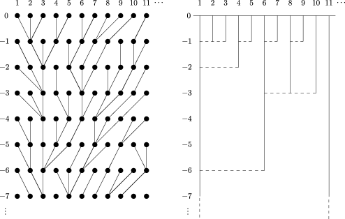
Figure 1: A doubly infinite embedding of quasi-stationary Bienaymé–Galton–Watson genealogies. Horizontal labels are individuals and vertical labels are generations. Left panel: the complete embedding of an infinite BGW tree. Right panel: coalescence times between consecutive individuals of generation 0. Here, the coalescent point process takes the value $(1,1,2,1,6,1,3,1,3,\ldots)$.

We are interested in having an arbitrarily large population at the present time, that we think of as generation 0, arising from a general branching process, originating at an unspecified arbitrarily large time in the past. In order to keep track of genealogies of individuals in the present population, for discrete Bienaymé–Galton–Watson (BGW) branching processes we use a representation that labels individuals at each generation in such a way that lines of descent of the population at any time do not intersect (see Figure 1). This leads to a monotone planar embedding of BGW trees such that each individual is represented by $(n,i)$ where $n\in\mathbb{Z}$ is the generation number and $i\in\mathbb{N}$ is the individual’s index in the generation. We consider BGW trees which are doubly infinite, allowing the number of individuals alive at present time to be arbitrarily large, and considering an infinite number of generations for their ancestry back in time. This monotone representation can also be extended to the case of continuous-state branching processes (later called CSB processes), in terms of a linearly ordered planar embedding of the associated genealogical $\mathbb{R}$-trees. This is in some way implicit in many recent works: our embedding is the exact discrete analogue of the flow of subordinators defined in BLG ; also, in the genealogy of CSB processes defined in LGLJ , the labeling of individuals at a fixed generation is analogous to the successive visits of the height process at a given level.

From our discrete embedding of the population, a natural consequence is that coalescence times, or times backwards to the most recent common ancestor, between individuals $k$ and $\ell$ in generation $0$, are represented by the maximum of the values $A_{i},i=k,\ldots,\ell-1$, where $A_{i}$ is the coalescence time between individuals $i$ and $i+1$. The genealogy back in time of the present population is then uniquely determined by the process $(A_{i};i\geq 1)$, which we call the branch lengths of the coalescent point process. In the continuous-state branching process setting, the $A_{i}$’s are given by depths of the excursions of the height process below the level representing the height of individuals in the present population.

In general, the process $(A_{i};i\geq 1)$ is not Markovian and its law is difficult to characterize. Our key strategy is to keep track of multiple ancestries to get a Markov process, thus constructing a coalescent point process with multiplicities $(B_{i};i\geq 1)$. Intuitively, for each $i\geq 1$, $B_{i}$ encodes the relationship of the individual $i+1$ to the infinite spine of the first present individual, by recording the nested sequence of subtrees that form that ancestral lineage linking $i+1$ to the spine. The value of $B_{i}$ is a point mass measure, where each point mass encodes one of these nested subtrees: the level of the point mass records the level back into the past at which this subtree originated, while the multiplicity of the point mass records the number of subtrees with descendants in individuals $\{i+1,i+2,\ldots\}$ emanating at that level which are embedded on the right-hand side of the ancestral link of $i+1$ to the spine.

Formally, for both BGW and the CSB population, we proceed as follows. We define a process with values in the integer-valued measures on $\mathbb{N}$ or $\mathbb{R}_{+}$ (BGW or CSB, resp.) in a recursive manner, in such a way that $(B_{j};1\leq j\leq i)$ will give a complete record of the ancestral relationship of individuals $1\leq j\leq i$. Start with the left-most individual in the present population, $i=1$, and let $B_{1}$ have a point mass at $n$, where $-n$ is the generation of the last common ancestor of individuals $1$ and $2$, and have multiplicity $B_{1}(\{n\})$ equal to the number of times this ancestor will also appear as the last common ancestor for individuals ahead, with index $i\geq 1$. We then proceed recursively, so that at individual $i$ we take the point masses in $B_{i-1}$; we first make an adjustment in order to reflect the change in multiplicities due to the fact that the lineage of individual $i$ is no longer considered to be an individual ahead of the current one. We then add a record for the last common ancestor of individuals $i$ and $i+1$. If this is an ancestor that has already been recorded in $B_{i-1}$, we just let $B_{i}$ be the updated value of $B_{i-1}$. Otherwise, we let $B_{i}$ be the updated $B_{i-1}$ plus a new point mass at $n$, if $-n$ is the generation of this new last common ancestor, whose multiplicity $B_{i}(\{n\})$ is the number of times this new ancestor will appear as the last common ancestor for individuals ahead, with index $\geq i+1$ (e.g., in Figure 1 we will have $B_{1}=2\delta_{1},B_{2}=\delta_{1},B_{3}=\delta_{2},B_{4}=\delta_{1},B_{5}=\delta_{6},B_{6}=\delta_{1},B_{7}=2\delta_{3},B_{8}=\delta_{1}+\delta_{3},B_{9}=\delta_{3}$).

Once we have constructed the coalescent point process with multiplicities (in either the BGW or CSB case), we will show that $A_{i}$ can be recovered as the location of the nonzero point mass in $B_{i}$ with the smallest level, that is, $A_{i}=\inf\{n\dvtx B_{i}(\{n\})\neq 0\}$ (e.g., in Figure 1 we have $A_{1}=1,A_{2}=1,A_{3}=2$, $A_{4}=1$, $A_{5}=6,A_{6}=1,A_{7}=3,A_{8}=1,A_{9}=3$). More importantly, we prove that $(B_{i};i\geq 1)$ is a Markov process, and that, when going from individual $i$ to $i+1$, the transitions decrease the multiplicity of the point mass of $B_{i}$ at level $\inf\{n\dvtx B_{i}(\{n\})\neq 0\}$ by 1, and that, with a specified probability, a new random point mass is added at a random level that must be smaller than the smallest nonzero level in the updated version of $B_{i}$.

In order to use this construction for both BGW and the CSB population, our take on what constitutes the sequence of present individuals has to be different for the continuous CSB population from the simple one for the discrete BGW population. Since in the CSB case the present population size is not discrete, and there is an accumulation of immediate ancestors at times arbitrarily close to the present time, we have to discretize the present population by considering only the individuals whose last common ancestor occurs at a time at least an $\varepsilon$ amount below the present time, for an arbitrary $\varepsilon>0$. We will later show that we can obtain the law of the coalescent point process with multiplicities for the CSB population as a limit of a sequence of appropriately rescaled coalescent point processes with multiplicities for the BGW population for which we also use the same discretization process of the present population. At first it may seem surprising that these coalescents with multiplicities are Markov processes over the set of all or the $\varepsilon$-discretized set (BGW and CSB case, resp.) individuals at present time. Below we intuitively explain why this is the case by describing the two approaches for constructing them.

In the discrete case, we start by giving a related, easier to define process $(D_{i}$; $i\geq 1)$, taking values in the integer-valued sequences, whose first nonzero term is also at level $A_{i}$. For each $i$, the sequence $(D_{i}(n),n\geq 1)$ gives the number of younger offshoots at generation $-n$ embedded on the right-hand side of the ancestor of $i$. The trees sprouting from the younger offshoots are independent, and the law of a tree sprouting from a younger offshoot at generation $-n$ has the law of the BGW tree conditioned to survive at least $n-1$ generations. It turns out that $(D_{i};i\geq 1)$ is Markov, and we construct $(B_{i};i\geq 1)$ from it, show that it is Markov as well and give its transition law. In order to be able to deal with the conditioning of younger offshoots in a way that allows us later to pass to the limit, we introduce an integer-valued measure $\rho$ that takes the ancestor of individual $1$ at generation $-n$ and records as $\rho(\{n\})=\rho_{n}$ the number of all of its younger offshoots embedded on the right-hand side, and we call it the great-aunt measure. This measure gives a spine decomposition of the first survivor (individual $i=1$) in such a way that the law of the trees sprouting from the younger offshoots are still independent, but are no longer conditioned on survival.

In the continuous-state case, the great-aunt measure will be a measure $\rho^{0}$ on $\mathbb{R}_{+}$, and we will be able to define the genealogy thanks to independent CSB processes starting from the masses of the atoms of $\rho^{0}$. In the subcritical and critical cases, this can be done using a single path of a Lévy process with no negative jumps and Laplace exponent $\psi$. In the supercritical case a concatenation of excursion paths will have to be used. Using the continuous great-aunt measure $\rho^{0}$, we characterize the genealogy of an infinite CSB tree with branching mechanism $\psi$ via the height function $H^{\star}$ whose value at an individual in the population can be decomposed into the level on the infinite spine at which the subtree containing this individual branches off, and the relative height of this individual within its subtree. We construct $(B^{\varepsilon}_{i};i\geq 1)$ from the height process $H^{\star}$. Discretizing the population by considering only the points whose coalescence times are greater than some fixed $\varepsilon>0$, translates into considering only the excursions of $H^{\star}$ from level $0$ with a depth greater than $-\varepsilon$. From these excursions we can obtain the process $((A^{\varepsilon}_{i},N^{\varepsilon}_{i});i\geq 1)$ where $A^{\varepsilon}_{i}$ is the depth of the $i$th such excursion and $N^{\varepsilon}_{i}$ is the number of future excursions with the exact same depth. It turns out that a specific functional of this process is Markov, and we construct $(B^{\varepsilon}_{i};i\geq 1)$ from it, show that it is Markov as well and give its transition law.

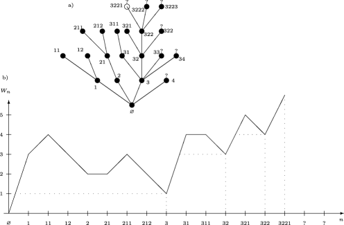
Figure 2: (a) A Bienaymé–Galton–Watson tree conditioned to have alive individuals at generation 4. The empty circle is the first such individual (3221) in the lexicographical order. Descendants of individuals with greater rank are only indicated by a question mark; (b) the associated random walk $W$ killed after the visit $\sigma_{4}$ of the first individual $x_{4}=3221$ with height 4. Records of the future infimum at $\sigma_{4}$ are shown by dotted lines. The record times are exactly the visits to ancestors $322,32,3$ and $\varnothing$ of 3221. The pairs of overshoots and undershoots of $W$ across the future infimum at those times (in this order) are $({\alpha}_{1},{\rho}_{1})=(0,2)$, $({\alpha}_{2},{\rho}_{2})=(1,1)$, $({\alpha}_{3},{\rho}_{3})=(1,2)$ and $({\alpha}_{4},{\rho}_{4})=(2,1)$.

Now, in order to prove convergence in law of the discretized version of $(B_{i}$; $i\geq 1)$ to $(B^{\varepsilon}_{i};i\geq 1)$, we make use of the great-aunt measures $\rho$ and $\rho^{0}$ describing the spine decomposition of the first surviving individual. In the discrete case, the spine decomposition $(\rho(\{n\});0\leq n\leq h)$ truncated at level $h$ has the same law as the spine decomposition of a planar embedding of a BGW tree conditioned on surviving up to generation $h$, where the first survivor is defined in the usual depth-first search order (see Figure 2). Using a well-known random walk representation of BGW trees BK , we then prove (under usual conditions ensuring the convergence of the random walk to a spectrally positive Lévy process $X$ with Laplace exponent $\psi$) the convergence (in the vague topology) of the great-aunt measure $\rho$ to the measure $\rho^{0}$ on $\mathbb{R}_{+}$ defined by

$$\rho^{0}(dx):=\beta\,dx+\sum_{t\dvtx\Delta_{t}>0}\Delta_{t}\delta_{t}(dx),$$

where $\beta$ is the Gaussian coefficient of $X$, and $(t,\Delta_{t})$ is a Poisson point measure with intensity

$$\biggl{(}e^{v(t)r}\int_{(r,\infty)}e^{-v(t)z}\Lambda(dz)\biggr{)}\,dt\,dr,\qquad r>0,$$

where $\Lambda$ is the Lévy measure of $X$, and $v$ the inverse of the decreasing function $\lambda\mapsto\int_{[\lambda,+\infty)}du/\psi(u)$. This is exactly the same measure $\rho^{0}$ we obtain from the spine decomposition in the continuous case. Since the transition law of $(B_{i};i\geq 1)$ can be represented as a functional of $\rho$ and the transition law of $(B^{\varepsilon}_{i};i\geq 1)$ as a functional of $\rho^{0}$, this will lead to our claim.

Finally, in the very last section, we give two simple applications of our results in the discrete case. First, we prove that in the linear-fractional case, the coalescent point process is a sequence of i.i.d. random variables. Related results can be found in Ran . Second, in the subcritical case, we use the monotone embedding to display the law, in quasi-stationary state, of the total population size (Yaglom’s limit) jointly with the time to most recent common ancestor of this whole population.

2 Doubly infinite embedding and the coalescent point process

2.1 The discrete model

We will start off with a monotone planar embedding of an infinitely old BGW process with arbitrarily large population size. Let $(\xi(n,i))$ be a doubly indexed sequence of integers, where $n$ is indexed by $\mathbb{Z}=\{\ldots,0,-1,-2,-3,\ldots\}$ and $i$ is indexed by $\mathbb{N}=\{1,2,3,\ldots\}$. The index pair $(n,i)$ represents the $i$th individual in generation $n$, and $\xi(n,i)$ provides the number of offspring of this individual.

We endow the populations with the following genealogy. Individual $(n,i)$ has mother $(n-1,j)$ if

$$\sum_{k=1}^{j-1}\xi(n-1,k)<i\leq\sum_{k=1}^{j}\xi(n-1,k).$$

From now on, we focus on the ancestry of the population at time 0, that we will call standing population, and we let $\mathfrak{a}_{i}(n)$ denote the index of the ancestor of individual $(0,i)$ in generation $-n$. In particular, $\mathfrak{a}_{i}(1):=\min\{j\geq 1\dvtx\sum_{k=1}^{j}\xi(-1,k)\geq i\}$. Our main goal is to describe the law of the times of coalescence $C_{i,j}$ of individuals $(0,i)$ and $(0,j)$, that is,

$$C_{i,j}:=\min\bigl{\{}n\geq 1\dvtx\mathfrak{a}_{i}(n)=\mathfrak{a}_{j}(n)\bigr{\}},$$

where it is understood that $\min\varnothing=+\infty$. Defining

$$A_{i}:=C_{i,i+1},$$

it is easily seen that by construction, for any $i\leq j$, $C_{i,j}=\max\{A_{i},A_{i+1},\ldots,\break A_{j-1}\}$. Thus, the sequence $A_{1},A_{2},\ldots$ contains all the information about the (unlabeled) genealogy of the current population and is called coalescent point process, as in P (see Figure 1).

We assume that there is a random variable $\xi$ with values in $\mathbb{Z}_{+}=\{0,1,2,\ldots\}$ and probability generating function (p.g.f.) $f$, such that all random variables (r.v.s) $\xi(n,i)$ are i.i.d. and distributed as $\xi$. As a consequence, if $Z^{(n,i)}(k)$ denotes the number of descendants of $(n,i)$ at generation $n+k$, then the processes $(Z^{(n,i)}(k);k\geq 0)$ are identically distributed Bienaymé–Galton–Watson (BGW) processes starting from 1. We will refer to $Z$ as some generic BGW process with this distribution and we will denote by $f_{n}$ the $n$th iterate of $f$ and by $p_{n}=1-f_{n}(0)$ the probability that $Z_{n}\not=0$. We need some extra notation in this setting.

We define $\zeta_{n}$ as the number of individuals at generation 1 having alive descendants at generation $n$. In particular, $\zeta_{n}$ has the law of

$$\sum_{k=1}^{\xi}\epsilon_{k},$$

where the $\epsilon_{k}$ are i.i.d. Bernoulli r.v.s with success probability $p_{n-1}$, independent of $\xi$. We also define $\zeta_{n}^{\prime}$ as the r.v. distributed as $\zeta_{n}-1$ conditional on $\zeta_{n}\not=0$.

2.2 The coalescent point process: Main results

Recall that $A_{i}$ denotes the time of coalescence of individuals $(0,i)$ and $(0,i+1)$, or $i$th branch length of the coalescent. To describe the law of $(A_{i};i\geq 1)$ we need an additional process.

Let $D_{i}(n)$ be the number of daughters of $(-n,\mathfrak{a}_{i}(n))$, distinct from $(-n+1$, $\mathfrak{a}_{i}(n-1))$, having descendants in $\{(0,j);j\geq i\}$. In other words, $D_{i}(n)$ is the number of younger surviving offshoots of $(-n,\mathfrak{a}_{i}(n))$ not counting the lineage of $(0,i)$ itself. Letting

$${\cal D}_{i}({n}):=\bigl{\{}\mbox{daughters of $\bigl{(}-n,\mathfrak{a}_{i}(n)\bigr{)}$ with descendants in $\bigl{\{}(0,j);j\geq i\bigr{\}}$}\bigr{\}},$$

we have

$$D_{i}(n)=\#{\cal D}_{i}({n})-1.$$

We set $D_{0}(n):=0$ for all $n$. We now provide the law of this process and its relationship to $(A_{i};i\geq 1)$. We also set $A_{0}:=+\infty$, which is in agreement with $\min\varnothing=+\infty$.

Theorem 2.1

The $i$th branch length is a simple functional of $(D_{i};i\geq 0)$

$$A_{i}=\min\bigl{\{}n\geq 1\dvtx D_{i}(n)\not=0\bigr{\}}.$$

In addition, the sequence-valued chain $(D_{i};i\geq 0)$ is a Markov chain started at the null sequence. For any sequence of nonnegative integers $(d_{n})_{n\geq 0}$, the law of $D_{i+1}$ conditionally given $D_{i}(n)=d_{n}$ for all $n$, is given by the following transition. We have $D_{i+1}(n)=d_{n}$ for all $n>A_{i}$, $D_{i+1}(A_{i})=d_{A_{i}}-1$ and the r.v.s $D_{i+1}(n)$, $1\leq n<A_{i}$, are independent, distributed as $\zeta_{n}^{\prime}$. In particular, the law of $A_{1}$ is given by

$$\mathbb{P}(A_{1}>n) = \prod_{k=1}^{n}\mathbb{P}\bigl{(}\zeta_{k}^{\prime}=0\bigr{)}=\frac{1}{1-f_{n}(0)}\prod_{k=1}^{n}f^{\prime}\bigl{(}f_{k-1}(0)\bigr{)}$$

$$= \frac{f_{n}^{\prime}(0)}{1-f_{n}(0)}=\mathbb{P}(Z_{n}=1\mid Z_{n}\not=0).$$

The following series of equivalences proves that $A_{i}$ is the level of the first nonzero term of the sequence $D_{i}$.

$$A_{i}>n\quad \Leftrightarrow \quad\forall k\leq n,\mathfrak{a}_{i}(k)\not=\mathfrak{a}_{i+1}(k)$$

$$\Leftrightarrow \quad\forall k\leq n,\forall j>i,\mathfrak{a}_{i}(k)\not=\mathfrak{a}_{j}(k)$$

$$\Leftrightarrow \quad\forall k\leq n,\bigl{(}-k,\mathfrak{a}_{i}(k)\bigr{)}\mbox{ has no descendants in }\bigl{\{}(0,j)\dvtx j>i\bigr{\}}$$

$$\Leftrightarrow \quad\forall k\leq n,D_{i}(k)=0.$$

Thanks to this last result, we get

$$\mathfrak{a}_{i}(A_{i})=\mathfrak{a}_{i+1}(A_{i})\quad\mbox{and}\quad\mathfrak{a}_{i}(A_{i}-1)\not=\mathfrak{a}_{i+1}(A_{i}-1).$$

In particular, $(-A_{i}+1,\mathfrak{a}_{i}(A_{i}-1))$ has no descendants in $\{(0,j)\dvtx j\geq i+1\}$, so that

$${\cal D}_{i+1}(A_{i})={\cal D}_{i}(A_{i})\setminus\bigl{\{}\bigl{(}-A_{i}+1,\mathfrak{a}_{i}(A_{i}-1)\bigr{)}\bigr{\}}$$

and $\#{\cal D}_{i+1}(A_{i})=\#{\cal D}_{i}(A_{i})-1$, that is, $D_{i+1}(A_{i})=D_{i}(A_{i})-1$.

Let us deal with the case $n>A_{i}$. By definition of $A_{i}$, $\mathfrak{a}_{i}(n)=\mathfrak{a}_{i+1}(n)$ for any $n\geq A_{i}$. As a consequence, for any $n>A_{i}$, each daughter of $(-n,\mathfrak{a}_{i+1}(n))$ has descendants in $\{(0,j);j\geq i+1\}$ iff she has descendants in $\{(0,j);j\geq i\}$. In other words, ${\cal D}_{i+1}(n)={\cal D}_{i}(n)$ and $D_{i+1}(n)=D_{i}(n)$.

Now we deal with the case $n<A_{i}$. Set

$$E_{i}:=\bigl{\{}D_{j}(n)=d_{j,n},\forall n\geq 1,j\leq i\bigr{\}},$$

where the $(d_{j,n})_{n\geq 1,j\leq i}$ are fixed integer numbers, and let ${A_{i}}$ be the value of the coalescence time of $i$ and $i+1$ conditional on $E_{i}$, that is, ${A_{i}}=\min\{n\geq 1\dvtx d_{i,n}\not=0\}$. Now let ${\cal T}(n,i)$ be the tree descending from $(-n,\mathfrak{a}_{i}(n))$ and set

$$I(n,i):=\min\bigl{\{}j\leq i\dvtx\mathfrak{a}_{j}(n)=\mathfrak{a}_{i}(n)\bigr{\}}.$$

Observe that the (unlabeled) tree ${\cal T}(n,i)$ has the law of a BGW tree conditioned on having at least one descendant at generation 0. Now, because the event $E_{i}$ only concerns the descendants of daughters of ancestors of $(-{A_{i}}+1,\mathfrak{a}_{i+1}({A_{i}}-1))$, the law of ${\cal T}({A_{i}}-1,i+1)$ conditional on $E_{i}$ is still the law of a BGW tree conditioned on having at least one descendant at generation 0.

Also notice that conditional on $E_{i}$, $I({A_{i}}-1,i+1)=i+1$. As a consequence, $I(n,i+1)=i+1$ for any $n<{A_{i}}$, so that for any $n<{A_{i}}$, conditional on $E_{i}$,

$${\cal D}_{i+1}(n):=\bigl{\{}\mbox{daughters of $\bigl{(}-n,\mathfrak{a}_{i+1}(n)\bigr{)}$ with descendants at generation 0}\bigr{\}}.$$

The result follows recalling the law of ${\cal T}({A_{i}}-1,i+1)$ conditional on $E_{i}$.

Recall that $D_{0}$ is a null sequence, $A_{0}=+\infty$, and that $D_{1}(n)\stackrel{{\scriptstyle d}}{{=}}\zeta^{\prime}(n)$ for $n\geq 1$. This infinite sequence of values in $\{D_{1}(n),n\geq 1\}$ contains information on the ancestral relationship of the individual $(0,1)$ and an arbitrarily large number of individuals in the standing population going back arbitrarily far into the past. Using the process $(D_{i};i\geq 1)$ we next define a sequence $(B_{i};i\geq 1)$ of finite point mass measures which contains the minimal amount of information needed to reconstruct $A_{1},A_{2},\ldots$ while remaining Markov. We do this for two reasons. First, if we are only interested in the ancestral relationship of finitely many individuals in the standing population, there is no need to keep track of an infinite sequence of values. Second, when we consider a rescaled limit of the BGW process to a CSB process, we will need to work with a sparser representation.

The main distinction between these two processes is that while $D_{i}$ contains information on the ancestral relationship of $(0,i)$ and $(0,j)$ for both $1\leq j\leq i+1$ and $j>i+1$, $B_{i}$ will only contain information about the ancestral relationship of $(0,i)$ and $(0,j)$ for $1\leq j\leq i+1$. In other words, if, say, $\max\{A_{1},\ldots,A_{i}\}=n$, then $B_{i}(m)=0$ for all $m>n$. Moreover, $B_{i}$ is defined directly from $D_{i}$ by letting $B_{i}(\{m\})=D_{i}(m)$ for all $m\leq n$. In particular, $B_{1}$ will have a single nonzero point mass at level $A_{1}$, and $B_{1}(\{A_{1}\})=D_{1}(A_{1})$.

We are now ready to define $(B_{i};i\geq 1)$ which we call the coalescent point process with multiplicities. Let $(B_{i};i\geq 0)$ be a sequence of finite point measures, started at the null measure, defined from $(D_{i};i\geq 0)$ recursively as follows. For any point measure $b=\sum_{n\geq 1}b_{n}\delta_{n}$, let $\mathfrak{s}(b)$ denote the minimum of the support of $b$, that is,

$$\mathfrak{s}(b):=\min\{n\geq 1\dvtx b_{n}\neq 0\}$$

with the convention that $\mathfrak{s}(b)=+\infty$ if $b$ is the null measure. If $B_{i}=\break\sum_{n\geq 1}b_{n,i}\delta_{n}$ for some $\{b_{n,i}\}_{n\geq 1}\in\mathbb{N}$, let

$$a_{1,i}:=\mathfrak{s}(B_{i}),\qquad B_{i}^{*}:=B_{i}-\delta_{a_{1,i}},\qquad a_{1,i}^{*}:=\mathfrak{s}\bigl{(}B_{i}^{*}\bigr{)}.$$

Then, define

$$B_{i+1}:=\cases{B_{i}^{*}+D_{i+1}(A_{i+1})\delta_{A_{i+1}},&\quad if $A_{i+1}<a_{1,i}^{*}$ and $A_{i+1}\neq a_{1,i}$,\vspace*{1pt}\cr B_{i}^{*},&\quad otherwise.}$$

Note that by Theorem 2.1 we have $D_{i+1}(A_{i})=D_{i}(A_{i})-1$, so by this definition $B_{i+1}=\sum_{n\geq 1}b_{n,i+1}\delta_{n}$, where $\{b_{n,i+1}\}_{n\geq 1}\in\mathbb{N}$ satisfies

$$b_{n,i+1}:=\cases{D_{i+1}(n),&\quad if $n$ is such that $b_{n,i}\neq 0$,\cr D_{i+1}(A_{i+1}),&\quad if $n=A_{i+1}$ and $A_{i+1}<a_{1,i}^{*}$ and $A_{i+1}\neq a_{1,i}$,\cr 0,&\quad for all other $n$.}$$

Roughly, $(B_{i};i\geq 1)$ records the ancestral information in the following way. $B_{0}$ is a null measure, and $B_{1}$ will contain a single point mass $B_{1}=D_{1}(A_{1})\delta_{A_{1}}$ recording the coalescence time $A_{1}$ for individuals $(0,1)$ and $(0,2)$ in the location of its point mass. Since the last common ancestor of $(0,1)$ and $(0,2)$ may also be the last common ancestor of $(0,1)$, $(0,2)$ and some other individual $(0,j)$ for $j\geq 2$, the multiplicity of this point mass will record the number of its future appearances in the coalescent point process. Recursively in every step, say $i+1$, this record of point masses will need to be updated from $B_{i}$ to $B^{*}_{i}$, since by moving one individual to the right we are no longer recording the last common ancestor of two previous individuals, and the number of future appearances of their last common ancestor by definition goes down by $1$. In addition, at step $i+1$ we also need to record the coalescence time for the last common ancestor of $(0,i+1)$ and $(0,i+2)$ with the number of its future appearances. This is done by taking the updated version $B^{*}_{i}$ and adding a new point mass $D_{i+1}(A_{i+1})\delta_{A_{i+1}}$ to create $B_{i+1}$. Because of the monotone embedding of the BGW as a planar tree, it is not possible for the level $A_{i+1}$ of this new point mass to be greater than any of the common ancestors of $(0,j)$ and $(0,k)$ for $1\leq j<k\leq i+1$ unless the multiplicities of these ancestors are depleted at this step and no longer appear in the updated $B^{*}_{i}$ (so $A_{i+1}\leq a^{*}_{1,i}$) as will be seen in the proof of the next theorem. Moreover, if the last common ancestor of $(0,i+1)$ and $(0,i+2)$ is the last common ancestor of $(0,i+1)$ and $(0,k)$ for some $1\leq k\leq i+1$, then the common ancestry of $(0,i+2)$ and $(0,i+1)$ will be counted in the multiplicity of the mass at $A_{i+1}$ in $B_{i}$ and the updated version $B^{*}_{i}$ will have nonzero multiplicity at $A_{i+1}$ (so $A_{i+1}=a^{*}_{1,i}$) and there will be no need to add a new point mass to create $B_{i+1}$. In addition, if this ancestor is also the last common ancestor of $(0,i)$ and $(0,i+1)$ (so $A_{i+1}=a_{1,i}$), the count for this ancestor cannot be 1 in $B_{i}$, so in this case we have $A_{i+1}=a_{1,i}=a^{*}_{1,i}$ and there is no need to add a new point mass in $B_{i+1}$.

We now provide the law of this point measure process and its relationship to $(A_{i};i\geq 1)$.

Theorem 2.2

The $i$th branch length is the smallest point mass in $B_{i}$

$$A_{i}=\mathfrak{s}(B_{i})=\min\bigl{\{}n\geq 1\dvtx B_{i}\bigl{(}\{n\}\bigr{)}\neq 0\bigr{\}}.$$

In addition, the sequence of finite point measures $(B_{i};i\geq 0)$ is a Markov chain started at the null measure, such that for any finite point measure $b=\sum_{n\geq 1}b_{n}\delta_{n}$, with $b_{n}\in\mathbb{N}\cup\{0\}$, the law of $B_{i+1}$ conditionally given $B_{i}=b$, is given by the following transition. Let $a_{1}:=\mathfrak{s}(b)$, $b^{*}:=b-\delta_{a_{1}}$ and $a_{1}^{*}:=\mathfrak{s}(b^{*})$. Let $(A,N)$ be distributed as $(A_{1},\zeta^{\prime}_{A_{1}})$. Then

$$B_{i+1}:=\cases{b^{*}+N\delta_{A},&\quad if $A<a_{1}^{*}$ and $A\neq a_{1}$,\cr b^{*},&\quad otherwise.}$$

Instead of the full information $(D_{1}(n),n\geq 1)$, this sequence starts with a single point measure

$$B_{1}=D_{1}(A_{1})\delta_{A_{1}},$$

and at each step it proceeds by changing the weights of the existing point masses and by adding at most one new point mass.

It is clear from the recursive definition of $(B_{i};i\geq 1)$ that for any $i\geq 1$ if $b_{n,i}\neq 0$, then $b_{n,i}=D_{i}(n)$. We first show that for any $i\geq 1$ we have $a_{1,i}=A_{i}$ and $b_{a_{1,i},i}=D_{i}(A_{i})$. If we show that $b_{A_{i},i}\neq 0$, then, since all other nonzero weights in $B_{i}$ satisfy $b_{n,i}=D_{i}(n)$, the definition of $A_{i}$ will immediately imply that $a_{1,i}=A_{i}$ and $b_{a_{1,i},i}=D_{i}(A_{i})$. We do this by induction. The claim is clearly true for $i=1$, so let us assume it is true for an arbitrary $i\geq 1$.

Consider what the transition rule for $D_{i}$ tells us about the relationship between $A_{i+1}$ and $A_{i}$. Recall for all $n>A_{i}$ we have $D_{i+1}(n)=D_{i}(n)$, $D_{i+1}(A_{i})=D_{i}(A_{i})-1$, and for all $n<A_{i}$ we have $D_{i+1}(n)=\zeta^{\prime}_{n}$ from r.v.s drawn independently of $D_{i}$. So,

$$A_{i+1}<A_{i}\quad \Leftrightarrow \quad\exists n<A_{i}\mbox{ s.t. }\zeta_{n}^{\prime}\neq 0,$$

$$A_{i+1}=A_{i}\quad \Leftrightarrow \quad D_{i}(A_{i})>1\mbox{ and }\zeta^{\prime}_{n}=0,\forall n<A_{i},$$

$$A_{i+1}>A_{i}\quad \Leftrightarrow \quad D_{i}(A_{i})=1\mbox{ and }\zeta^{\prime}_{n}=0,\forall n<A_{i}.$$

In the first case, $A_{i+1}<A_{i}=a_{1,i}\leq a_{1,i}^{*}$, so the point mass at $A_{i+1}$ will be added to $B_{i+1}$ and $b_{A_{i+1},i+1}\neq 0$. In the second case, $b_{A_{i},i+1}=D_{i+1}(A_{i})=D_{i}(A_{i})-1>0$, and since $A_{i+1}=A_{i}$, we have $b_{A_{i+1},i+1}\neq 0$. In the third case, $b_{A_{i},i+1}=D_{i+1}(A_{i})=D_{i}(A_{i})-1=0$, and also $b_{a_{1,i},i}=D_{i}(A_{i})=1$ implies $a_{1,i}^{*}=\min\{n>a_{1,i}\dvtx b_{n,i}\neq 0\}=\min\{n>A_{i}\dvtx b_{n,i}\neq 0\}$. Note that for all $n>A_{i}$ for which $b_{n,i}\neq 0$, we also have $b_{n,i+1}=b_{n,i}\neq 0$, and since $b_{A_{i},i+1}=0$, the smallest value of $n$ with mass $B_{i+1}(\{n\})>0$ before we potentially add a new mass is precisely at $a_{1,i}^{*}=\min\{n>A_{i}\dvtx b_{n,i}\neq 0\}$. In this case $a_{1,i}^{*}>a_{1,i}=A_{i}$ so we have $D_{i+1}(a_{1,i}^{*})=D_{i}(a_{1,i}^{*})\neq 0$, so by definition of $A_{i+1}$ we must have $A_{i+1}\leq a_{1,i}^{*}$. In case $A_{i+1}<a_{1,i}^{*}$, the point mass at $A_{i+1}$ will be added to $B_{i+1}$ and $b_{A_{i+1},i+1}\neq 0$. In case $A_{i+1}=a_{1,i}^{*}$, no new mass is added and the smallest of the nonzero masses in $B_{i+1}$ is at $a_{1,i}^{*}=A_{i+1}$, as stated earlier, and again $b_{A_{i+1},i+1}=b_{a_{1,i}^{*},i+1}=b_{a_{1,i}^{*},i}\neq 0$. Hence, we have shown by induction that $b_{A_{i},i}\neq 0$ for all $i\geq 1$, so that $a_{1,i}=A_{i}$ and $b_{a_{1,i},i}=B(A_{i},i)$.

Now consider the transition rule for $B_{i+1}$, conditionally given $B_{i}$. For the already existing mass in $B_{i}$ the changes in weights are given by the transition rule for $D_{i}$ to be

$$\sum_{n\geq 1}D_{i+1}(n)\mathbf{1}_{\{b_{n,i}\neq 0\}}\delta_{n} = \bigl{(}D_{i}(A_{i})-1\bigr{)}\delta_{A_{i}}+\sum_{n>A_{i}}D_{i}(n)\mathbf{1}_{\{b_{n,i}\neq 0\}}\delta_{n}$$

$$= B_{i}-\delta_{a_{1,i}}=B_{i}^{*}.$$

We have an addition of a new point mass iff $A_{i+1}<a_{1,i}^{*}$. Since $a_{1,i}^{*}\geq a_{1,i}=A_{i}$, this happens iff either: [(ii)]

$A_{i+1}<A_{i}$, or

$b_{a_{1,i},i}=1$ and $A_{i}<A_{i+1}<a_{1,i}^{*}$. The reason $A_{i}=A_{i+1}$ is not included in (ii) is that if $b_{a_{1,i},i}=D_{i}(A_{i})=1$ then $D_{i+1}(A_{i})=D_{i}(A_{i})-1=0$. Let $\{\zeta^{\prime}_{n}\}_{n\geq 1}$ be a sequence of r.v.s drawn independently from $D_{i}$. Then, by the transition rule for $D_{i}$: [(ii)]

holds iff $\exists n<A_{i}$ s.t. $\zeta_{n}^{\prime}\neq 0$, then, $A_{i+1}:=\min\{n<A_{i}\dvtx\zeta_{n}^{\prime}\neq 0\}$;

holds iff $b_{a_{1,i},i}=1$, $\forall n<A_{i}$ $\zeta^{\prime}_{n}=0$ and $\exists n<a_{1,i}^{*}$ s.t. $\zeta^{\prime}_{n}\neq 0$, then, $A_{i+1}:=\min\{A_{i}<n<a_{1,i}^{*}\dvtx\zeta_{n}^{\prime}\neq 0\}$.

In case (i) holds it is clear that the weight $D_{i+1}(A_{i+1})$ is distributed as $\zeta^{\prime}_{A_{1}}$ conditional on $A_{1}<A_{i}=a_{1,i}^{*}$ and that this weight is independent of $(B_{j};1\leq j\leq i)$. We next argue that this is also true in case (ii) holds. In this case $A_{i}<A_{i+1}<a_{1,i}^{*}$ and since $D_{i+1}(A_{i+1})\neq 0$ we must also have $D_{i}(A_{i+1})\neq 0$ because the transition rule for $D_{i+1}$ only allows zero entries to become nonzero for $n<A_{i}$. Moreover, $D_{i}(A_{i+1})=D_{i+1}(A_{i+1})$ because all entries for $n>A_{i}$ remain unchanged from step $i$ to $i+1$. Hence, we must have $D_{n}(A_{i+1})=D_{i+1}(A_{i+1})$ for all $k<n\leq i$ where

$$k:=\max\{0\leq j<i\dvtx A_{j}\geq a_{1,i}^{*}\}$$

with the convention that $A_{0}:=+\infty$.

We show that $A_{k}\neq A_{i+1}$ if $A_{i}<A_{i+1}<a_{1,i}^{*}$. If we had $A_{k}=A_{i+1}$, then $b_{A_{k},k}=D_{k}(A_{k})\neq 0$. The transition rule for $D_{k+1}$ implies $D_{k+1}(A_{k})=\break D_{k}(A_{k})-1$. Since $A_{n}<A_{i+1}=A_{k}$ for all $k+1\leq n\leq i$, iteratively applying the transition rule for $D_{k+2},\ldots,D_{i+1}$ implies $D_{k+2}(A_{k})=D_{k+1}(A_{k}),\ldots,\break D_{i+1}(A_{k})=D_{i}(A_{k})$. Thus

$$D_{k}(A_{k})-1=D_{k+1}(A_{k})=\cdots=D_{i}(A_{k})=D_{i+1}(A_{k})=D_{i+1}(A_{i+1})\neq 0$$

and $b_{A_{k},k}=D_{k}(A_{k})>1$. Then, by definition of the weights for $B_{k+1},\ldots,B_{i+1}$, we have that $b_{A_{k},k+1}=D_{k+1}(A_{k})\neq 0$ and the same weight iteratively remains as $b_{A_{k},n}=D_{n}(A_{k})$ for all $k+1\leq n\leq i+1$. However, $b_{A_{i+1},i}=b_{A_{k},i}\neq 0$ contradicts our assumption that $A_{i+1}<a_{1,i}^{*}$.

Thus we must have $A_{k}>A_{i+1}$. Since $D_{i}(A_{k})\neq 0$ we also must have $A_{k}\geq a_{1,i}^{*}$. From the definition of weights for $B_{i}$ and $A_{i}<a_{1,i}^{*}$ we have

$$b_{a_{1,i}^{*},i}\neq 0\quad\Rightarrow\quad\exists k^{\prime}<i\mbox{ s.t. }a_{1,i}^{*}=A_{k^{\prime}}\mbox{ and }A_{n}<A_{k^{\prime}}\mbox{ for all }k^{\prime}<n\leq i$$

since the only point mass in a step $n$ not existing in the previous step must be placed at $A_{n}$. Now, $A_{k^{\prime}}=a_{1,i}^{*}>A_{i+1}$ and the fact that we defined $k=\max\{0\leq j<i\dvtx A_{j}\geq A_{i+1}\}$ implies that $k=k^{\prime}$, hence, $A_{k}=a_{1,i}^{*}$.

Since $A_{k}>A_{i+1}$, we must have $D_{k}(A_{i+1})=0$. By the same argument as above of iteratively applying the transition rule for $D_{k+2},\ldots,D_{i+1}$, the weights at $A_{i+1}$ satisfy

$$D_{k+1}(A_{i+1})=\cdots=D_{i}(A_{i+1})=D_{i+1}(A_{i+1})\neq 0.$$

Let us now consider the distribution of $D_{i+1}(A_{i+1})$ conditional on the value of $k$. Since $A_{i+1}<A_{k}$ and $D_{k+1}(A_{i+1})\neq 0$ by the transition rule for $D_{k+1}$, the value of the weight $D_{k+1}(A_{i+1})$ is a r.v. distributed as $\zeta^{\prime}_{A_{1}}$ conditional on $A_{1}<A_{k}$ and it is drawn independently of $(B_{j};1\leq j\leq k)$. So, $D_{i+1}(A_{i+1})=D_{k+1}(A_{i+1})$ is distributed as $\zeta^{\prime}_{A_{1}}$ conditional on $A_{1}<A_{k}=a_{1,i}^{*}$ and is independent of $(B_{j};1\leq j\leq k)$. Since $A_{n}<A_{i+1}$ for all $k<n\leq i$, the transition rule for $D_{k+1},\ldots,D_{i}$ implies that all of the subsequently added point masses in $B_{k+1},\ldots,B_{i}$ are independent of $D_{k+1}(A_{i+1})$, so the value of $D_{i+1}(A_{i+1})$ is independent of $(B_{j};1\leq j\leq i)$. Finally, integrating over $k$, we have that $D_{i+1}(A_{i+1})$ is distributed as $\zeta^{\prime}_{A_{1}}$ conditional on $A_{1}<a_{1,i}^{*}$ and is independent of $(B_{j};1\leq j\leq i)$.

We have now shown that when a new point mass is added at $A_{i+1}$, either $A_{i+1}:=\min\{n<A_{i}\dvtx\zeta_{n}^{\prime}\neq 0\}$, or $b_{a_{1,i},i}=1$ and $A_{i+1}:=\min\{A_{i}<n<a_{1,i}^{*}\dvtx\zeta_{n}^{\prime}\neq 0\}$, where the sequence $\{\zeta^{\prime}_{n}\}_{n\geq 1}$ are r.v.s drawn independently from $(B_{j};j\leq i)$. In either case, the weight of the new point mass at $A_{i+1}$ is distributed as $\zeta^{\prime}_{A_{1}}$ conditional on $A_{1}<a_{1,i}^{*}$.

Let $A:=\min\{n\geq 1\dvtx\zeta^{\prime}_{n}\neq 0\}$ and $N:=\zeta^{\prime}_{A}$. Since $\{\zeta^{\prime}_{n}\}_{n\geq 1}$ are independent of $(B_{j};1\leq j\leq i)$, so are $A$ and $N$, and by Theorem 2.1, $(A,N)$ is distributed as $(A_{1},\zeta^{\prime}_{A_{1}})$. Conditional on the value of $B_{i}$, we have that (i) holds iff $A<A_{i}$, while (ii) holds iff $b_{a_{1,i},i}=1$ and $A_{i}<A<a_{1,i}^{*}$. Putting (i) and (ii) together with the definition of $a_{1,i}^{*}$ we have, conditionally on $(B_{j};1\leq j\leq i)$, an addition of a new point mass iff $A<a_{1,i}^{*}$ and $A\neq a_{1,i}$. Moreover, the weight of the newly added point mass is distributed as $\zeta^{\prime}_{A_{1}}$ conditional on $A_{1}<a_{1,i}^{*}$, or equivalently it is distributed as $N$ conditional on $A<a_{1,i}^{*}$. We also showed that given $(B_{j};1\leq j\leq i)$, the point masses existing in $B_{i}$ change in the next step to produce a re-weighted point mass measure equal to $B_{i}-\delta_{a_{1}}$. Altogether, given $(B_{j};1\leq j\leq i)$, the next step of the sequence depends on $B_{i}$ only, with the transition rule that if $A<a_{1,i}^{*}$ and $A\neq a_{1,i}$ in the next step we have $B_{i+1}=B_{i}-\delta_{a_{1,i}}+N\delta_{A}$, and otherwise in the next step we have $B_{i+1}=B_{i}-\delta_{a_{1,i}}$.

In the course of the above proof, we have also shown that if $t_{1}:=\min\{t\geq 1\dvtx A_{t}>A_{1}\}$ and $N_{1}:=\#\{1\leq j<t_{1}\dvtx A_{j}=A_{1}\}$, then $N_{1}=D_{1}(A_{1})$, because in order to add the first new point mass at a level greater than $A_{1}$, we must in the course of $1\leq j<t_{1}$ have exactly enough steps at which $A_{j}=A_{1}$ that will exhaust all of the weight $D_{1}(A_{1})$ of the point mass at $A_{1}$.

Analogously for each $i\geq 1$, if we let

$$t_{i}:=\min\{t\geq i\dvtx A_{t}>A_{i}\}\quad\mbox{and}\quad N_{i}:=\#\{i\leq j<t_{i}\dvtx A_{j}=A_{i}\},$$

then $D_{i}(A_{i})=N_{i}$. If, furthermore, for each $i\geq 1$ and $k\geq i$ we define

$$N_{ik}:=\#\{k\leq j<t_{i}\dvtx A_{j}=A_{i}\},$$

then by a similar argument for $k\geq i$ we have $N_{ik}=D_{k}(A_{i})$. Note that $N_{ii}\equiv N_{i}$. Then, for the sequence of finite point measures we have that for all $k\geq 1$,

$$B_{k}=\sum_{i\leq k}N_{ik}\delta_{A_{i}}\mathbf{1}_{\{A_{i}<A_{i^{\prime}},\forall{i^{\prime}}<i\dvtx N_{{i^{\prime}}k}\neq 0\}}.$$ (1)

It is easily checked that $B_{k+1}$ correctly updates the weight of each existing point mass from $B_{k}$, and allows a new point mass to be added only if it is in a location smaller than all mass existing in $B_{k}$ whose weights in $B_{k+1}$ remain nonzero. We will see this formula again when we discuss the coalescent process in the continuous case.

Remark 1.

In the discrete case the coalescence times $A_{i}$ take on integer values which may occur again after they have appeared for the last time $t_{i}$ in a subtree. In the continuous case, analogously defined coalescence times have a law that is absolutely continuous w.r.t. Lebesgue measure, their values a.s. never occur again after they have appeared for the last time in a subtree, hence, in the continuous case there is no need to use separation times $t_{i}$ in the definition of counters $N_{i}$ and $N_{ik}$.

3 From discrete to continuous: The great-aunt measure

3.1 Definition of the great-aunt measure

Now that we have a simple description of the coalescent point process with multiplicities for a BGW branching process, our goal is to do the same for the continuous-state branching process. In the discrete case we used the process $(D_{i};i\geq 1)$ to describe the number of surviving younger offshoots of ancestors of an individual as a sequence indexed by generations backward in time. Since in the CSB case the standing population is not discrete, we cannot use a process indexed by the standing population. Instead, we use a spine decomposition of the lineage of a surviving individual, which will record the level (i.e., generation in the discrete, and height in the continuous case) and the number of all offshoot subtrees in the individual’s genealogy. We first provide the law of the spine decomposition of the first individual in the standing population in the BGW case and relate it to our previous results. At this point we would like to emphasize that results for the spine decomposition of BGW process are not new (see references at the end of the subsection), and that we make use of the spine decomposition here only as a tool that will enable us to describe the analogue of the coalescent point process with multiplicities for the CSB process later.

We give some new definitions to describe the spine decomposition of $(0,1)$, the first individual in generation $0$, of a BGW process within its monotone planar embedding. For $n\geq 1$, we denote by $\phi_{n}$ the set of great-aunts of $(0,1)$ at generation $-n+1$, that is,

$$\phi_{n}:=\bigl{\{}\mbox{daughters of }\bigl{(}-n,\mathfrak{a}_{1}(n)\bigr{)}\mbox{ excluding }\bigl{(}-n+1,\mathfrak{a}_{1}(n-1)\bigr{)}\bigr{\}},$$

and by $\varphi_{n}$ its cardinal, $\varphi_{n}:=\#\phi_{n}$. In other words, $\varphi_{n}$ is the number of offshoots of $(-n,\mathfrak{a}_{1}(n))$ not counting the lineage of $(0,1)$ itself. The set $\phi_{n}$ can be divided into

$$\alpha_{n}:=\bigl{\{}\mbox{sisters of }\bigl{(}-n+1,\mathfrak{a}_{1}(n-1)\bigr{)}\mbox{ with labels }(-n+1,k)\mbox{ s.t. }k<\mathfrak{a}_{1}(n-1)\bigr{\}}$$

the older offshoots of $(-n,\mathfrak{a}_{1}(n))$, and

$$\rho_{n}:=\bigl{\{}\mbox{sisters of }\bigl{(}-n+1,\mathfrak{a}_{1}(n-1)\bigr{)}\mbox{ with labels }(-n+1,k)\mbox{ s.t. }k>\mathfrak{a}_{1}(n-1)\bigr{\}}$$

the younger offshoots of $(-n,\mathfrak{a}_{1}(n))$. We call the sequence $(\rho_{n};n\geq 1)$ the great-aunt measure. We let $(Z_{k}^{\alpha_{n}};0\leq k\leq n-1)$ and $(Z_{k}^{\rho_{n}};0\leq k\leq n-1)$ be the processes counting the descendants of those $\alpha_{n}$ and $\rho_{n}$ individuals, respectively, at successive generations $-n+1,\ldots,0$.

An important observation now is that we do not need the whole infinite embedding of trees to make the previous definitions. The descending tree of $(-h,\mathfrak{a}_{1}(h))$ is a planar BGW tree conditioned to have alive individuals at generation $h$, with the lineage of individual $(0,1)$ being the left-most lineage with alive descendants at generation $h$. Consequently, provided that we only consider indices $n\leq h$, our definitions make sense for any conditioned BGW planar tree. A number of results have already been proved in Gei2 for spine decomposition of BGW process conditioned on survival at a given generation, and we make use of them here. The infinite embedding of trees that we introduced extends these results in a way, as we are considering an arbitrarily large standing population that may not [in (sub)critical case] descend from the same ancestor $n$ generations back in the past. Considering trees whose roots are individuals $(-n,\mathfrak{a}_{1}(n)),(-n,\mathfrak{a}_{1}(n)+1),\ldots\,$, it is easy to see that they are independent and identically distributed as ${\cal T}(n,1)$, the tree descending from $(-n,\mathfrak{a}_{1}(n))$.

We recall some standard notation commonly used with linearly ordered planar trees. The Ulam–Harris–Neveu labeling of a planar tree assumes that each individual (vertex) of the tree is labeled by a finite word $u$ of positive integers whose length $|u|$ is the generation, or height, of the individual. A rooted, linearly ordered planar tree ${\cal T}$ is a subset of the set ${\cal U}$ of finite words of integers

$${\cal U}=\bigcup_{n\geq 0}\mathbb{N}^{n},$$

where $\mathbb{N}^{0}$ is the empty set. More specifically, the root of $\cal T$ is denoted $\varnothing$ and her offspring are labeled $1,2,3,\ldots$ from left to right. The recursive rule is that the offspring of any individual labeled $u$ are labeled $u1,u2,u3,\ldots$ from left to right, where $ui$ is the mere concatenation of the word $u$ and the number $i$. The depth-first search is the lexicographical order associated with Ulam–Harris–Neveu labeling (see Figure 2, where the depth-first search gives the order $\varnothing,1,11,12,2,211,212,3,31,311,32,\ldots$).

Now fix $h\in\mathbb{N}$ and assume that generation $h$ is nonempty. Let $x_{h}$ be the Ulam–Harris–Neveu label of the first individual in depth-first search with height $h$. We denote by $(x_{h}\mid-n)$ the ancestor of $x_{h}$ at generation $h-n$. Then for $1\leq n\leq h$, we can define $\alpha^{\prime}_{n}$ and $\rho^{\prime}_{n}$ to be the number of daughters of $(x_{h}\mid-n)$ ranked smaller and larger, respectively, than $(x_{h}\mid-n+1)$, and define $\varphi^{\prime}_{n}:=\alpha^{\prime}_{n}+\rho^{\prime}_{n}$. We can also let $Z^{\alpha^{\prime}_{n}}$ and $Z^{\rho^{\prime}_{n}}$ be the processes counting the descendants of those $\alpha^{\prime}_{n}$ and $\rho^{\prime}_{n}$ individuals, respectively. From now on, we assume that the tree $\cal T$ has the law of a planar BGW tree with offspring distributed as $\xi$ and conditioned to have alive individuals at generation $h$. Then it is easily seen that $(\alpha^{\prime}_{n},\rho^{\prime}_{n},Z^{\alpha^{\prime}_{n}}\circ\mathrm{k}_{n},Z^{\rho^{\prime}_{n}}\circ\mathrm{k}_{n};1\leq n\leq h)$ (where $\mathrm{k}_{n}$ means killing at time $n$) has the same distribution as $(\alpha_{n},\rho_{n},Z^{\alpha_{n}},Z^{\rho_{n}};1\leq n\leq h)$, so from now on we remove primes. The following result provides the joint law of these random variables, which was already shown in Gei2 , and the results below are just a restatement of Lemma 2.1 from Gei2 . Recall that $p_{n}=\mathbb{P}(Z_{n}\not=0\mid Z_{0}=1)$.

Proposition 3.1.

Conditional on the values of $(\alpha_{n},\rho_{n};n\geq 1)$, the processes $(Z^{\alpha_{n}},Z^{\rho_{n}};n\geq 1)$ are all independent, $Z^{\rho_{n}}$ is a copy of $Z$ started at $\rho_{n}$ and killed at time $n$ and $Z^{\alpha_{n}}$ is a copy of $Z$ started at $\alpha_{n}$, conditioned on being zero at time $n-1$. In addition, the pairs $(\alpha_{n},\rho_{n};n\geq 1)$ are independent and distributed as follows:

$$\mathbb{P}(\alpha_{n}=j,\varphi_{n}=k)=\mathbb{P}(\xi=k+1)\frac{p_{n-1}}{p_{n}}(1-p_{n-1})^{j},\qquad k\geq j\geq 0.$$

Remark 2.

Recall that $D_{1}(n)$ is the number of sisters of $(-n+1,\mathfrak{a}_{1}(n-1))$ with alive descendants in the standing population. Thus, an immediate corollary of Proposition 3.1 is that the random variables $(D_{1}(n);n\geq 1)$ are independent and that, conditionally on $\rho_{n}$, $D_{1}(n)$ is a binomial r.v. with parameters $\rho_{n}$ and $p_{n-1}$. Since, according to Theorem 2.1, $D_{1}(n)$ is distributed as $\zeta^{\prime}_{n}$, we also have

$$\mathbb{E}\bigl{(}s^{\zeta^{\prime}_{n}}\bigr{)}=\mathbb{E}\bigl{(}(1-p_{n-1}+p_{n-1}s)^{\rho_{n}}\bigr{)}$$

as one can easily check.

Note that the last statement in Proposition 3.1 can be viewed as an inhomogeneous spine decomposition of the “ascendance” of the surviving particles in conditioned BGW trees. More standard spine decompositions are well known for the “descendance” of conditioned branching trees (see, e.g., Ev , L-PTRF , L-EJP , LPP , Gei1 , CRW , K ) (the idea of spine decompositions originating from K ). To bridge the gap between both aspects, notice that in the (sub)critical case, $\mathbb{P}(\varphi_{n}+1=k)=\mathbb{P}(\xi=k)(1-(1-p_{n-1})^{k})/p_{n}$ converges to $k\mathbb{P}(\xi=k)/\mathbb{E}(\xi)$ as $n\to\infty$, which is the size-biased distribution of $\xi$. This distribution is known to be the law of offspring sizes on the spine when conditioning the tree on infinite survival.

3.2 A random walk representation

We next show how to recover any truncation $(\rho_{n};n\leq h)$ of the great-aunt measure from the paths of a conditioned, killed random walk. This will be particularly useful when we define the analogue of the great-aunt measure for continuous-state branching processes in the next subsection. Our result makes use of a well-known correspondence between a BGW tree and a downward-skip-free random walk introduced and studied in BK , LGLJ .

Let us go back to the planar tree $\cal T$. We denote by $v_{n}$ the word labeling the $n$th individual of the tree in the depth-first search. For any integers $i>j$ and any finite word $u$, we say that $ui$ is “younger” than $uj$. Also, we will write $u\prec v$ if $u$ is an ancestor of $v$, that is, there is a sequence $w$ such that $v=uw$ (in particular, $u\prec u$). Last, for any individual $u$ of the tree, we let $r(u)$ denote the number of younger sisters of $u$, and for any integer $n$, we let $W_{n}:=0$ if $v_{n}=\varnothing$, and if $v_{n}$ is any individual of the tree different from the root, we let

$$W_{n}:=\sum_{u\prec v_{n}}r(u).$$

The height $H_{n}$, or generation, of the individual visited at time $n$ can be recovered from $W$ as

$$H_{n}:=|v_{n}|=\#\Bigl{\{}1\leq k\leq n\dvtx W_{k}=\min_{k\leq j\leq n}W_{j}\Bigr{\}}.$$ (2)

See Figure 2 where $(W_{n};n=1,\ldots,15)$ is given until visit of $v_{15}=3221$ whose height is $H_{15}=4$.

In the case when $\cal T$ is a BGW tree with offspring distributed as $\xi$, then it is known BK , LGLJ that the process $(W_{n};n\geq 1)$ is a random walk started at 0, killed upon hitting $-1$, with steps in $\{-1,0,1,2,\ldots\}$ distributed as $\xi-1$.

Fix $h\in\mathbb{N}$ and set

$$\sigma_{h}:=\min\{n\geq 1\dvtx H_{n}=h\}.$$

Writing $T_{j}$ for the first hitting time of $j$, in particular, $T_{-1}$ for the first hitting time of $-1$, we get

$$\Bigl{\{}\max_{0\leq j\leq T_{-1}}H_{j}<h\Bigr{\}}=\{Z_{h}=0\}=\{\sigma_{h}\geq T_{-1}\}.$$ (3)

Now, when $\sigma_{h}<T_{-1}$, we let $I_{\sigma_{h}}$ denote the future infimum process of the random walk killed at $\sigma_{h}$

$$I_{\sigma_{h}}^{j}:=\min_{j\leq r\leq\sigma_{h}}W_{r},$$

and we let $t_{h}=0,\ldots,t_{0}=\sigma_{h}$ denote the successive record times of $I_{\sigma_{h}}$

$$t_{k}:=\max\bigl{\{}j<t_{k-1}\dvtx W_{j}=I_{\sigma_{h}}^{j}\bigr{\}},\qquad 1\leq k\leq h.$$

Also observe that by definition of $\sigma_{h}$, we must have $t_{1}=t_{0}-1$. Last, we use the notation $\Delta_{j}W:=W_{j+1}-W_{j}$. A straightforward consequence of BK , LGLJ is that when generation $h$ is nonempty, $t_{k}$ is the visit time of $(x_{h}\mid-k)$, that is, the unique integer $n$ such that $v_{n}=(x_{h}\mid-k)$ (where $x_{h}$ is the first individual in depth-first search with height $h$). Furthermore,

$$\varphi_{k}=\Delta_{t_{k}}W=W_{t_{k}+1}-W_{t_{k}}$$

and

$$\alpha_{k}=W_{t_{k}+1}-\min_{t_{k}+1\leq j\leq t_{0}}W_{j}\quad\mbox{and}\quad\rho_{k}=\min_{t_{k}+1\leq j\leq t_{0}}W_{j}-W_{t_{k}}.$$

In particular, we can check ${\alpha}_{1}=0$, and ${\varphi}_{k}={\alpha}_{k}+{\rho}_{k}$. Now note that, by definition of $t_{h},\ldots,t_{0}$, we have $I^{t_{k}}_{\sigma_{h}}=W_{t_{k}}$ and for all $j\dvtx t_{k}<j<t_{k-1}$ we have $I^{j}_{\sigma_{h}}=W_{t_{k-1}}$, so

$${\alpha}_{k}=W_{t_{k}+1}-I^{t_{k}+1}_{\sigma_{h}}=W_{t_{k}+1}-W_{t_{k-1}}\quad\mbox{and}\quad{\rho}_{k}=I^{t_{k}+1}_{\sigma_{h}}-W_{t_{k}}=W_{t_{k-1}}-W_{t_{k}}.$$

An illustration of these claims can be seen in Figure 2.

Last, observe that

$$\sum_{k=1}^{h}{\rho}_{k}f(k) = \sum_{k=1}^{h}\bigl{(}I_{\sigma_{h}}^{t_{k}+1}-W_{t_{k}}\bigr{)}f(k)=\sum_{k=1}^{h}\sum_{j=0}^{\sigma_{h}-1}{\mathbf{1}}_{j=t_{k}}\bigl{(}I_{\sigma_{h}}^{j+1}-W_{j}\bigr{)}f(h-H_{j})$$

$$= \sum_{j=0}^{\sigma_{h}-1}\Delta_{j}I_{\sigma_{h}}^{j}f(h-H_{j})$$

since, if $j=t_{k}$ for some $k$, then

$$\Delta_{j}I^{j}_{\sigma_{h}}=\Delta_{t_{k}}I^{t_{k}}_{\sigma_{h}}=I^{t_{k}+1}_{\sigma_{h}}-I^{t_{k}}_{\sigma_{h}}=I^{t_{k}+1}_{\sigma_{h}}-W_{t_{k}},$$

otherwise, $t_{k}<j<t_{k-1}$ for some $k$, and

$$\Delta_{j}I^{j}_{\sigma_{h}}=I^{j+1}_{\sigma_{h}}-I^{j}_{\sigma_{h}}=W_{t_{k-1}}-W_{t_{k-1}}=0.$$

This is recorded in the following statement, which we will use later as a distributional equality for a random walk $W$ conditioned on $\max_{1\leq j\leq T_{-1}}H_{j}\geq h$.

Proposition 3.2.

For any $f\dvtx\mathbb{N}\longrightarrow\mathbb{R}_{+}$ with bounded support,$h>\operatorname{Supp}(f)$, if $\max_{1\leq j\leq T_{-1}}H_{j}\geq h$, then

$$\langle\rho,f\rangle:=\sum_{k\geq 1}\rho_{k}f(k)=\sum_{j=0}^{\sigma_{h}-1}\Delta_{j}I_{\sigma_{h}}^{j}f(h-H_{j}),$$

where $\Delta_{j}I_{\sigma_{h}}^{j}=I_{\sigma_{h}}^{j+1}-I_{\sigma_{h}}^{j}$.

3.3 A continuous version of the great-aunt measure

In Section 2, we gave a consistent way of embedding trees with an arbitrary size of the standing population, each descending from an arbitrarily old founding ancestor, so that the descending subtree of each vertex is a BGW tree. The natural analog of this presentation is the flow of subordinators introduced by Bertoin and Le Gall in BLG . Because the Poissonian construction of this flow displayed in BLG3 , Section 2, only holds for critical CSB processes and without Gaussian component, and because it is rather awkward to use in order to handle the questions we address here, we will now define an analogue of the great-aunt measure, using the genealogy of continuous-state branching processes introduced in LGLJ and further investigated in DLG .

We start with a Lévy process $X$ with no negative jumps and Laplace exponent $\psi$ started at $x>0$, such that $\psi^{\prime}(0+)\geq 0$, so that $X$ hits 0 a.s. As specified in L1 , L2 , the path of $X$ killed upon reaching 0 can be seen as the (jumping) contour process of a continuous tree whose ancestor is the interval $(0,x)$. For example, the excursions of $X$ above its past infimum $I$ are the contour processes of the offspring subtrees of the ancestor. Almost surely for all $t$, it is possible to define the height (i.e., generation) $H_{t}$ of the point of the tree visited at time $t$, as

$$H_{t}:=\lim_{k\to\infty}\frac{1}{\varepsilon_{k}}\int_{0}^{t}{\mathbf{1}}_{\{X_{s}<I_{t}^{s}+\varepsilon_{k}\}}\,ds<\infty,$$ (4)

where $(\varepsilon_{k})$ is some specified vanishing positive sequence, and

$$I_{t}^{s}:=\inf_{s\leq r\leq t}X_{r}.$$

With this definition, one can recover the population size at generation $a$ as the density $Z_{a}$ of the occupation measure of $H$ at $a$, that is, the (total) local time of $H$ at level $a$. It is proved in LGLJ , DLG that this local time exists a.s. for all $a$ and that $(Z_{a};a\geq 0)$ is a continuous-state branching process with branching mechanism $\psi$.

From now on, we will deal with a general branching mechanism $\psi$ characterized by its Lévy–Khinchin representation

$$\psi(\lambda)=a\lambda+\beta\lambda^{2}+\int_{(0,\infty)}\Lambda(dr)\bigl{(}e^{-\lambda r}-1+\lambda r{\mathbf{1}}_{\{r<1\}}\bigr{)},$$

where $\beta>0$ is the Gaussian component and $\Lambda$ is a positive measure on $(0,\infty)$ such that $\int_{(0,\infty)}(1\wedge r^{2})\Lambda(dr)<\infty$, called the Lévy measure. We will denote by $X$ a Lévy process with Laplace exponent $\psi$ (started at 0 unless otherwise stated), and by $Z$ a continuous-state branching process, or CSB process, with branching mechanism $\psi$.

We (only) make the following two assumptions. First,

$$\sup\bigl{\{}\lambda\dvtx\psi(\lambda)\leq 0\bigr{\}}=:\eta<\infty,$$

so that $X$ is not a subordinator (i.e., it is not a.s. nondecreasing). Second,

$$\int_{[\eta+1,\infty)}\frac{du}{\psi(u)}<\infty,$$

so that $Z$ either is absorbed at 0 in finite time or goes to $\infty$, and $H$ has a.s. continuous sample paths LGLJ . This also forces $\int_{(0,1)}r\Lambda(dr)$ to be infinite, so that the paths of $X$ have infinite variation. We further set

$$\phi(\lambda):=\int_{[\lambda,\infty)}\frac{du}{\psi(u)},\qquad\lambda>\eta,$$

and $v$ the inverse of $\phi$ on $(\eta,+\infty)$

$$v(x):=\phi^{-1}(x),\qquad x\in(0,\infty).$$

Notice that $v$ is nonincreasing and has limit $\eta$ at $+\infty$. It is well known (e.g., L1 ) that if $Z$ is started at $x$, then it is absorbed at 0 before time $t$ with probability $e^{-xv(t)}$. Also, if $N$ denotes the excursion measure of $X-I$ away from 0 under $\mathbb{P}$ (normalized so that $-I$ is the local time), then by DLG , Corollary 1.4.2,

$$N(\sup H>a)=v(a),\qquad a>0.$$

Here, we want to allow the heights of the tree to take negative values. To do this, we start with a measure which embodies the mass distribution broken down on heights, of the population whose descendances have not yet been visited, in the same vein as in LGLJ , DLG , but with negative heights. In the usual setting, the mass distribution $\rho_{t}$ of the population whose descendances have not yet been visited by the contour process $X$ by time $t$, is defined by

$$\langle\rho_{t},f\rangle=\int_{[0,t]}d_{s}I_{t}^{s}f(H_{s})$$

for any nonnegative function $f$, where on the right-hand side we mean integrating the function $s\mapsto f(H_{s})$ with respect to the Stieltjes measure associated with the function $s\mapsto I_{t}^{s}$. Then $\rho_{t}([a,b])$ is the mass of the tree between heights $a$ and $b$ whose descendants have not yet been visited by the contour process.

Here, we will start with a random positive measure $\rho^{0}$ on $[0,+\infty)$, with the interpretation that $\rho^{0}([a,b])$ is the mass of the tree between heights $-b$ and $-a$ whose descendants have not yet been visited by the contour process. This measure is the exact analogue of the great-aunt measure of the previous subsection.

Definition 3.3.

For every $t>0$, set $\pi^{(t)}(dr):=p(t,r)\,dr$, where

$$p(t,r):=e^{v(t)r}\int_{(r,\infty)}e^{-v(t)z}\Lambda(dz),\qquad r>0.$$

We define $\rho^{0}$ in law by

$$\rho^{0}(dx):=\beta\,dx+\sum_{t\dvtx\Delta_{t}>0}\Delta_{t}\delta_{t}(dx),$$

where $\delta$ denotes a Dirac measure, and $(t,\Delta_{t})$ is a Poisson point measure with intensity measure $dt\,\pi^{(t)}(dr)$.

3.4 Convergence of the great-aunt measure

We can now prove a theorem yielding two justifications for the definition of the measure $\rho^{0}$. First, we show that $\rho^{0}(dx)$ as defined above is indeed the mass, at height $h-x$, of the part of the tree whose descendants have not yet been visited, either by a long-lived contour process ($h\to\infty$) or under the measure $N(\cdot\mid\sup H>h)$. Second, we show the convergence of the appropriately re-scaled discrete great-aunt measures to the measure $\rho^{0}$, as the BGW processes approach the CSB process $Z$ with branching mechanism $\psi$. In the next section we will show how $\rho^{0}$ allows us to define the coalescent point process with multiplicities for the CSB process, and help us establish convergence from the appropriately re-scaled point process $(B_{i};i\geq 1)$.

We assume there exists a sequence $(\gamma_{p};p\geq 1)$, $\gamma_{p}\to\infty$ as $p\to\infty$, and a sequence of random variables $(\xi_{p};p\geq 1)$, such that, if $W^{(p)}$ denotes the random walk with steps distributed as $\xi_{p}-1$, the random variables $(p^{-1}W^{(p)}_{[p\gamma_{p}]})$ converge in law to $X_{1}$, where $X$ denotes the Lévy process with Laplace exponent $\psi$. Then it is known (Gri , Theorems 3.1 and 3.4) that if $Z^{(p)}$ denotes the BGW process started at $[px]$ with offspring size distributed as $\xi_{p}$, then the re-scaled processes $(p^{-1}Z^{(p)}_{[\gamma_{p}t]};t\geq 0)$ converge weakly in law in Skorokhod space to the CSB process $Z$ with branching mechanism $\psi$, started at $x$.

In the following statement, we denote by $\rho^{(p)}$ the great-aunt measure associated to the offspring size $\xi_{p}$. We have to make the following additional assumptions: if $f^{(p)}$ denotes the p.g.f. of $\xi_{p}$ and $f^{(p)}_{n}$ its $n$th iterate, then for each $\delta>0$,

$$\mathop{\lim\inf}_{p\to\infty}f^{(p)}_{[\delta\gamma_{p}]}(0)^{p}>0.$$

Convergence results in (iii) below rely heavily on results already established by Duquesne and Le Gall in DLG on convergence of appropriately re-scaled random walks $W^{(p)}$ and their height processes $H^{(p)}$ to the Lévy process $X$ and its height process $H$. In particular, technical conditions such as the one above are justified in DLG , Section 2.3.

Theorem 3.4

Let $\sigma_{h}$ denote the first time that $H$ hits $h>0$. [(iii)]

For any $h>0$ and for any nonnegative Borel function $f$ vanishing outside $[0,h]$, the random variable $\int_{[0,{\sigma_{h}}]}d_{s}I_{\sigma_{h}}^{s}f(h-H_{s})$, under $N(\cdot\mid\sup H>h)$, has the same law as $\langle\rho^{0},f\rangle$;

For any nonnegative Borel function $f$ with compact support, as $h\to\infty$ the random variables $\int_{[0,{\sigma_{h}}]}d_{s}I_{\sigma_{h}}^{s}f(h-H_{s})$ under $\mathbb{P}(\cdot\mid\sigma_{h}<\infty)$ converge in distribution to $\langle\rho^{0},f\rangle$;

For any nonnegative Borel function $f$ with compact support and sequence of nonnegative continuous functions $\{f_{p}\}$ such that $f_{p,\gamma_{p}}(x_{p}):=f_{p}(\gamma_{p}^{-1}x_{p})\to f(x)$ whenever $\gamma_{p}^{-1}x_{p}\to x$, the random variables $p^{-1}\langle\rho^{(p)},f_{p,\gamma_{p}}\rangle$ converge in distribution to $\langle\rho^{0},f\rangle$ as $p\to\infty$.

Let us prove (i). It is known DLG that a.s. for all $t$ the inverse of the local time on $[0,t]$ of the set of increase times of $(I_{t}^{s};s\in[0,t])$ has drift coefficient $\beta$, so that

$$\int_{[0,t]}d_{s}I_{t}^{s}f(H_{s})=\beta\int_{0}^{H_{t}}f(x)\,dx+\sum_{s\in[0,t]}f(H_{s})\Delta_{s}I_{t}^{s},$$

where the sum is taken over all times $s$ at which $(I_{t}^{s};s\in[0,t])$ has a jump, whose size is then denoted $\Delta_{s}I_{t}^{s}$. This set of times will be denoted ${\cal J}_{h}$ when $t=\sigma_{h}$. As a consequence, it only remains to prove that the random point measure $M_{h}$ on $(0,h)\times(0,\infty)$ defined by

$$M_{h}:=\sum_{s\in{\cal J}_{h}}\delta\bigl{(}H_{s},\Delta_{s}I_{\sigma_{h}}^{s}\bigr{)},$$

where the sum is zero when ${\cal J}_{h}$ is empty ($\sigma_{h}=\infty$), is an inhomogeneous Poisson point measure with the correct intensity measure. More precisely, we are going to check that for any nonnegative two-variable Borel function $f$

$$N\biggl{(}\int_{(0,h)\times(0,\infty)}M_{h}(dt\,dr)f(h-t,r)\Bigm{|}\sup H>h\biggr{)}=\int_{0}^{h}dt\int_{0}^{\infty}dr\,p(t,r)f(t,r),$$

that is,

$$N\int_{(0,h)\times(0,\infty)}M_{h}(dt\,dr)f(h-t,r)=v(h)\int_{0}^{h}dt\int_{0}^{\infty}dr\,p(t,r)f(t,r).$$

First notice that

$$N\int_{(0,h)\times(0,\infty)}M_{h}(dt\,dr)f(h-t,r)$$

$$\qquad=N\sum_{s\dvtx\Delta X_{s}>0}{\mathbf{1}}_{s<\sigma_{h}}f\bigl{(}h-H_{s},\Delta X_{s}+K_{s}^{\prime}\bigr{)}{\mathbf{1}}_{\Delta X_{s}>-K_{s}^{\prime}},$$

where $K_{s}^{\prime}$ is the global infimum of the shifted path $X^{\prime}$

$$X^{\prime}_{u}:=X_{s+u}-X_{s},\qquad 0\leq u\leq\sigma_{h}-s.$$

But on $\{s<\sigma_{h}\}$, $\sigma_{h}-s$ is also $\sigma^{\prime}_{h-H_{s}}$ (with obvious notation), so by predictable projection and by the compensation formula applied to the Poisson point process of jumps, we get

$$N\int_{(0,h)\times(0,\infty)}M_{h}(dt\,dr)f(h-t,r)=N\int_{0}^{\sigma_{h}}ds\int_{(0,\infty)}\Lambda(dz)G_{f}(z,H_{s}),$$

where (with the notation $I$ for the current infimum)

$$G_{f}(z,t)=\mathbb{E}_{0}\bigl{[}f(h-t,z+I_{\sigma_{h-t}}){\mathbf{1}}_{-I_{\sigma_{h-t}}<z}\bigr{]}.$$

Now $-I_{\sigma_{h-t}}$ is the local time at the first excursion of $X-I$ with height larger than $h-t$ so it is exponentially distributed with parameter $N(\sup H>h-t)=v(h-t)$. As a consequence,

$$G_{f}(z,t)=v(h-t)\int_{0}^{z}drf(h-t,r)e^{-(z-r)v(h-t)},$$

which yields

$$N\int_{(0,h)\times(0,\infty)}M_{h}(dt\,dr)f(h-t,r)=N\int_{0}^{\sigma_{h}}ds\,F_{f}(h-H_{s})$$

with

$$F_{f}(t) = \int_{(0,\infty)}\Lambda(dz)G_{f}(z,h-t)$$

$$= v(t)\int_{(0,\infty)}\Lambda(dz)\int_{0}^{z}dr\,f(t,r)e^{-(z-r)v(t)}$$

$$= v(t)\int_{0}^{\infty}dr\,f(t,r)e^{rv(t)}\int_{(r,\infty)}\Lambda(dz)e^{-zv(t)}$$

$$= v(t)\int_{0}^{\infty}dr\,p(t,r)f(t,r).$$

So we only have to verify that for any nonnegative Borel function $g$,

$$N\int_{0}^{\sigma_{h}}ds\,g(h-H_{s})=\int_{0}^{h}dt\,\frac{v(h)}{v(t)}g(t).$$

Due to results in LGLJ , there indeed is a jointly measurable process $(Z(a,t);\break a,t\geq 0)$ such that a.s. for all $a$,

$$\int_{0}^{a}ds\,g(H_{s})=\int_{0}^{\infty}dt\,Z(a,t)g(t).$$

In particular,

$$N\int_{0}^{\sigma_{h}}ds\,g(h-H_{s})=\int_{0}^{h}dt\,N\bigl{(}Z(\sigma_{h},t)\bigr{)}g(h-t),$$

so we just need to check that $N(Z(\sigma_{h},t))={v(h)}/{v(h-t)}$, that is,

$$N\bigl{(}Z(\sigma_{h},t)\mid\sup H>h\bigr{)}=\frac{1}{v(h-t)}.$$

But, conditional on $\sup H>h$, $\sigma_{t}<\infty$ and $Z(\sigma_{h},t)$ is the local time of $H$ at level $t$ between $\sigma_{t}$ and $\sigma_{h}$, which is exponential with parameter $N(\sup H>h-t)=v(h-t)$, hence, the claimed expectation.

We proceed with (ii), which readily follows from (i). Indeed, for any $h$ larger than $\sup\{x\dvtx f(x)\not=0\}$,

$$\int_{[0,{\sigma_{h}}]}d_{s}I_{\sigma_{h}}^{s}f(h-H_{s})=\int_{[0,{\sigma_{h}}]}d_{s}I_{\sigma_{h}}^{s\prime}f\bigl{(}h-H_{s}^{\prime}\bigr{)},$$

where primes indicate that the future infimum and the height process are taken w.r.t. the process $X^{\prime}$ with law $N(\cdot\mid\sup H>h)$, defined as

$$X^{\prime}_{t}=X_{{\rho_{h}}+t}-I_{\sigma_{h}},\qquad 0\leq t\leq\tau_{h}-\rho_{h},$$

where $\rho_{h}$ is the unique time $s\leq\sigma_{h}$ when $X_{s}=I_{\sigma_{h}}$ and $\tau_{h}$ is the first time $t\geq\sigma_{h}$ when $X_{t}=I_{\sigma_{h}}$.

We end the proof with (iii). Thanks to Proposition 3.2, we know that $\langle\rho^{(p)},f_{p,\gamma_{p}}\rangle$ has the same law as

$$\sum_{j=0}^{[\sigma^{p}_{\gamma_{p}h}]}\Delta I^{(p)j}_{\sigma^{p}_{\gamma_{p}h}}f_{p,\gamma_{p}}\bigl{(}\gamma_{p}h-H^{(p)}_{j}\bigr{)}$$

conditional on $\max_{1\leq j\leq T^{(p)}_{-1}}H^{(p)}_{j}\geq\gamma_{p}h$, where $H^{(p)}$ is the height process associated with $W^{(p)}$, $T^{(p)}_{-1}$ is the first hitting time of $-1$ by $W^{(p)}$, $\sigma^{p}_{\gamma_{p}h}$ denotes the first hitting time of $\gamma_{p}h$ by $H^{(p)}$ and $I^{(p)}$ denotes the future infimum process of $W^{(p)}$ stopped at time $\sigma^{p}_{\gamma_{p}h}$. If we can prove convergence of $(p^{-1}W^{(p)}_{[p\gamma_{p}\cdot\land\sigma^{p}_{\gamma_{p}h}]},\gamma_{p}^{-1}H^{(p)}_{[p\gamma_{p}\cdot\land\sigma^{p}_{\gamma_{p}h}]})$ under this conditional law to $(X_{\cdot\land\sigma_{h}},H_{\cdot\land\sigma_{h}})$ under the measure $N(\cdot\mid\sup H\geq h)$, then by the generalized continuous mapping theorem (e.g., Kal , Theorem 4.27) we will get the convergence of

$$\sum_{j=0}^{[\sigma^{p}_{\gamma_{p}h}]}\frac{\Delta I^{(p)j}_{\sigma^{p}_{\gamma_{p}h}}}{p}f_{p}\biggl{(}h-\frac{H^{(p)}_{j}}{\gamma_{p}}\biggr{)},$$

which has the law of $p^{-1}\langle\rho^{(p)},f_{p,\gamma_{p}}\rangle$, to $\int_{[0,{\sigma_{h}}]}d_{s}I_{\sigma_{h}}^{s}f(h-H_{s})$ under $N(\cdot\mid\sup H>h)$ which has the law of $\langle\rho^{0},f\rangle$ thanks to (i).

For (sub)critical $\xi_{p}$ the convergence of this pair in distribution on the Skorokhod space of cadlag real-valued paths is a direct consequence of the results Corollary 2.5.1 and Proposition 2.5.2 already shown in DLG , Section 2.5. To verify that the same holds for supercritical $\xi_{p}$ as well, we note that the assumption of (sub)criticality (hypothesis (H2) in the notation of DLG ) is not crucial in any of the steps of their proof, since the obtained convergence relies essentially only on the assumption that $p^{-1}W^{(p)}_{[p\gamma_{p}\cdot]}$ converges to $X$ (see the comment in the proof of Theorem 2.2.1 in DLG that any use of subcriticality in their proof can be replaced by using weak convergence of random walks). Of course, in the supercritical case, the height process $H$ may drift off to infinity corresponding to the event that the CSB process $Z$ survives forever, in which case it will code only an incomplete part of the genealogy of the first lineage which survives forever. However, for our purposes we only need to consider the genealogy of the first lineage that survives until time $h$, so this will not be an impediment for our considerations.

For supercritical $\xi_{p}$ we still have the convergence of the pair

$$\bigl{(}p^{-1}W^{(p)}_{[p\gamma_{p}\cdot]},\gamma_{p}^{-1}H^{(p)}_{[p\gamma_{p}\cdot]}\bigr{)}\mathop{\longrightarrow}^{d}_{p\to\infty}(X_{\cdot},H_{\cdot})$$ (5)

in distribution on the Skorokhod space of cadlag real-valued paths as in Theorem 2.3.1 and the first part of Corollary 2.5.1 in DLG , Section 2.5. We now follow the same reasoning as in DLG , Proposition 2.5.2. Let $G^{p}_{\gamma_{p}h}=\sup\{s\leq\sigma^{p}_{\gamma_{p}h}\dvtx H^{(p)}_{s}=0\}$. If we think of $H^{(p)}$ as the height process for a sequence of independent BGW trees with offspring distribution $\xi_{p}$, then $G^{p}_{\gamma_{p}h}$ is the initial point of the first BGW tree in this sequence which reaches a height $\gamma_{p}h$. Let $(\tilde{W}{}^{(p)},\tilde{H}{}^{(p)})$ denote the process obtained by conditioning $(W^{(p)},H^{(p)})$ on $\max_{1\leq j\leq T^{(p)}_{-1}}H^{(p)}_{j}\geq\gamma_{p}h$. Then,

$$\bigl{(}p^{-1}\tilde{W}{}^{(p)}_{[p\gamma_{p}\cdot\land\sigma^{p}_{\gamma_{p}h}]},\gamma_{p}^{-1}\tilde{H}{}^{(p)}_{[p\gamma_{p}\cdot\land\sigma^{p}_{\gamma_{p}h}]}\bigr{)}$$

$$\qquad\stackrel{{\scriptstyle d}}{{=}}\bigl{(}p^{-1}W^{(p)}_{[p\gamma_{p}(G^{p}_{\gamma_{p}h}+\cdot)\land\sigma^{p}_{\gamma_{p}h}]},\gamma_{p}^{-1}H^{(p)}_{[p\gamma_{p}(G^{p}_{\gamma_{p}h}+\cdot)\land\sigma^{p}_{\gamma_{p}h}]}\bigr{)}.$$

Let $G_{h}=\sup\{s\leq\sigma_{h}\dvtx H_{s}=0\}$, and let $(\tilde{X},\tilde{H})$ denote the process obtained by conditioning $(X,H)$ on $\sup H\geq h$, then

$$(\tilde{X}_{\cdot\land\sigma_{h}},\tilde{H}_{\cdot\land\sigma_{h}})\stackrel{{\scriptstyle d}}{{=}}(X_{(G_{h}+\cdot)\land\sigma_{h}},H_{(G_{h}+\cdot)\land\sigma_{h}}).$$

If we use the Skorokhod representation theorem to assume that the convergence (5) holds a.s., the same arguments as in proof Proposition 2.5.2 of DLG imply that $\sigma^{p}_{\gamma_{p}h}$ converges a.s. to $\sigma_{h}$ and $G^{p}_{\gamma_{p}h}$ converges a.s. to $G^{p}_{h}$, and hence, $(p^{-1}W^{(p)}_{[p\gamma_{p}(G^{p}_{\gamma_{p}h}+\cdot)\land\sigma^{p}_{\gamma_{p}h}]},\gamma_{p}^{-1}H^{(p)}_{[p\gamma_{p}(G^{p}_{\gamma_{p}h}+\cdot)\land\sigma^{p}_{\gamma_{p}h}]})$ converges a.s. to $(X_{(G_{h}+\cdot)\land\sigma_{h}},H_{(G_{h}+\cdot)\land\sigma_{h}})$, proving that

$$\bigl{(}p^{-1}\tilde{W}{}^{(p)}_{[p\gamma_{p}\cdot]},\gamma_{p}^{-1}\tilde{H}{}^{(p)}_{[p\gamma_{p}\cdot]}\bigr{)}\mathop{\longrightarrow}^{d}_{p\to\infty}(\tilde{X}_{\cdot},\tilde{H}_{\cdot})$$

in distribution on the Skorokhod space of cadlag real-valued paths. From this the desired convergence in distribution of $p^{-1}<\rho^{(p)},f_{p,\gamma_{p}}>$ conditional on $\max_{1\leq j\leq T^{(p)}_{-1}}H^{(p)}\geq\gamma_{p}h$ to $\langle\rho^{0},f\rangle$ under the measure $N(\cdot\mid\sup H\geq h)$ follows.

4 The coalescent point process in the continuous case

4.1 Definition of the genealogy

We now define the analogue of a coalescent point process with multiplicities for the genealogy (other than the immediately recent) of an arbitrarily large standing population of a CSB process $Z$. We do so by first constructing the height process, $H^{\star}$, for a planar embedding of CSB trees of arbitrary size descending from an arbitrarily old ancestor using the continuous version of the great-aunt measure, $\rho^{0}$. From $H^{\star}$ we define coalescence times of two masses from the standing population in the usual way, that is, from the maximal depths of the trajectory of $H^{\star}$.

We construct the height $H_{t}^{\star}$ of the individual visited at time $t$ from: the height $H_{t}$ defined in (4) representing the height at which that individual occurs in an excursion of $X$ above its infimum; plus the height at which this excursion branches off the unexplored part of the tree. More specifically, let

$$Y^{0}_{x}:=\rho^{0}\bigl{(}[0,x]\bigr{)},\qquad x\geq 0,$$

so that

$$Y^{0}_{x}=\beta x+\sum_{t\leq x}\Delta_{t},$$

where $(t,\Delta_{t})$ is a Poisson point measure with intensity given by $dt\,\pi^{(t)}(dr)$ from Definition 3.3. Next, let $L^{0}$ denote the right-inverse of $Y^{0}$,

$$L^{0}(t):=\inf\bigl{\{}a\dvtx Y_{a}^{0}>t\bigr{\}},\qquad t\geq 0.$$

Then define

$$H_{t}^{\star}:=H_{t}-L^{0}(-I_{t}),$$

where we remember that $I_{t}=\inf_{0\leq s\leq t}X_{s}$.

This gives a spine decomposition of the genealogy of the continuous-state branching process associated with $H^{\star}$ in the following sense. For the individual visited by the traversal process at time $t$, the level (measured back into the past, with the present having level $0$) on the infinite spine at which the subtree containing this individual branches off is $-L^{0}(-I_{t})$, and the relative height of this individual within this subtree is $H_{t}$.

As in the discrete case, we want to display the law of the coalescence time between successive individuals at generation 0. In this setting, this corresponds to the maximum depth below 0 of the height process, between successive visits of 0. Actually, any point at height 0 is a point of accumulation of other points at height 0, so we discretize the population at height 0 as follows. We consider all points at height 0 such that the height process between any two of them goes below $-\varepsilon$, for some fixed $\varepsilon>0$, namely, we set $T_{0}:=0$, and for any $i\geq 1$,

$$S_{i}:=\inf\bigl{\{}t\geq T_{i-1}\dvtx H_{t}^{\star}=-\varepsilon\bigr{\}}\quad\mbox{and}\quad T_{i}:=\inf\bigl{\{}t\geq S_{i}\dvtx H_{t}^{\star}=0\bigr{\}}.$$

Then the coalescence times $A_{1}^{\varepsilon},A_{2}^{\varepsilon},\ldots$ of the $\varepsilon$-discretized population are defined as

$$A_{i}^{\varepsilon}:=-\inf\bigl{\{}H_{t}^{\star}\dvtx T_{i-1}\leq t\leq T_{i}\bigr{\}}.$$ (6)

As in the discrete case, one of the main difficulties lies in the fact that the same value of $A_{i}^{\varepsilon}$ can be repeated several times. So we define

$$N_{i}^{\varepsilon}:=\#\bigl{\{}j\geq i\dvtx A_{j}^{\varepsilon}=A_{i}^{\varepsilon}\bigr{\}}.$$ (7)

4.2 The supercritical case

Actually, the previous definition of genealogy only holds for the subcritical and critical cases, and a modification needs to be made in the supercritical case due to possible appearances of branches with infinite survival times into the future. What we need to do in the supercritical case is construct a height process $H^{\star}$ that corresponds to a CSB tree whose infinite branches have been truncated, much as in the last chapter of L1 . One would be naturally led to consider the height process of a tree truncated at some finite height. However, the distribution of such an object is far more complicated than to truncate (actually, reflect) the associated Lévy process at some finite level. On the other hand, the genealogy coded by a Lévy process reflected below some fixed level is not easy to read since it will have incomplete subtrees at different heights. To comply with this difficulty, we will construct a consistent family of Lévy processes $X^{\kappa}$ reflected below level $\kappa$, so that if $\kappa^{\prime}>\kappa$, $X^{\kappa}$ can be obtained from $X^{\kappa^{\prime}}$ by excising the subpaths above $\kappa$. The genealogy coded by the projective limit of this family is the supercritical Lévy tree, as is shown in L1 in the case with finite variation. We first give the details of this construction in the discrete case and then sketch its definition in the CSB case. Let $\cal T$ be a planar, discrete, possibly infinite, tree in the sense that it can have infinite height but all finite breadths. Then $\cal T$ still admits a Ulam–Harris–Neveu labeling and, as in Section 3.2, we can define $\hat{W}(\varnothing)=0$ and

$$\hat{W}(v):=\sum_{u\prec v}r(u),\qquad u\not=\varnothing,$$

where $r(u)$ denotes the number of younger sisters of $u$. Now for any $\kappa\in\mathbb{N}$, let ${\cal T}^{\kappa}$ denote the graph obtained from $\cal T$ by deleting all vertices $v$ such that $\hat{W}(v)>\kappa$. It is then easy to see that ${\cal T}^{\kappa}$ is still a tree, and that if $v_{n}^{\kappa}$ denotes the $n$th vertex of ${\cal T}^{\kappa}$ in the lexicographical order and $W_{n}^{\kappa}:=\hat{W}(v_{n}^{\kappa})$, then for any $\kappa^{\prime}>\kappa$, the path of $W^{\kappa}$ can be obtained from the path of $W^{\kappa^{\prime}}$ by excising the subpaths above $\kappa$. In other words,

$$W^{\kappa}=C_{\kappa}\bigl{(}W^{\kappa^{\prime}}\bigr{)},$$

where for any path $\epsilon$, the functional $C_{\kappa}$ erasing subpaths above $\kappa$ can be defined as follows. Let $A^{\kappa}$ denote the additive functional

$$A_{n}^{\kappa}(\epsilon):=\sum_{k=0}^{n}{\mathbf{1}}_{\{\epsilon_{k}\leq\kappa\}},\qquad n\in\mathbb{N},$$

and $a^{\kappa}$ its right inverse

$$a_{k}^{\kappa}(\epsilon):=\min\bigl{\{}n\dvtx A_{n}^{\kappa}(\epsilon)>k\bigr{\}},\qquad k\in\mathbb{N}.$$

Then $C_{\kappa}(\epsilon):=\epsilon\circ a^{\kappa}(\epsilon)$.

Further, it can be shown that $W^{\kappa}$ has the law of the random walk with steps distributed as $\xi-1$, reflected below $\kappa$ and killed upon hitting $-1$. Since these two properties (consistency by truncation and marginal distribution) characterize the family of reflected, killed random walks $(W^{\kappa};\kappa\in\mathbb{N})$, its continuous analogue has the following natural definition.

For any $\kappa>0$ let $X^{\kappa}$ denote a Lévy process without negative jumps and Laplace exponent $\psi$ reflected below $\kappa$ and killed upon reaching 0. The reflection can be properly defined as follows. Start with the path of a Lévy process $X$ (with the same Laplace exponent), set $S_{t}:=\sup_{0\leq s\leq t}X_{s}$ and define $X^{\kappa}_{t}:=X_{t}$ if at time $t$, $X$ has not yet hit $(\kappa,+\infty)$, and $X_{t}^{\kappa}:=\kappa+X_{t}-S_{t}$ otherwise (and kill $X^{\kappa}$ when it hits 0). The same definition could be done by concatenating excursions of $X$ away from $(\kappa,+\infty)$ thanks to Itô’s synthesis theorem.

Now, in the continuous setting, a similar definition of $C_{\kappa}$ can be done by adapting the additive functional $A^{\kappa}$ into

$$A_{t}^{\kappa}(\epsilon):=\int_{0}^{t}ds\,{\mathbf{1}}_{\{\epsilon_{s}\leq\kappa\}},\qquad t\geq 0.$$

It is easily seen that for any $\kappa^{\prime}>\kappa$,

$$X^{\kappa}\stackrel{{\scriptstyle d}}{{=}}C_{\kappa}\bigl{(}X^{\kappa^{\prime}}\bigr{)}.$$

Kolmogorov’s extension theorem then ensures the existence of a family of processes $(X^{\kappa};\kappa>0)$ defined on the same probability space, satisfying pathwise the previous equality, and with the right marginal distributions (reflected, killed Lévy processes).

All results stated in the remainder of the paper hold in the supercritical case if we replace the Lévy process $X$ by the projective limit of $X^{\kappa}$ as $\kappa\to\infty$. More simply, we can construct the same consistent family $(e^{\kappa};\kappa>0)$ for the excursion of $X-I$ away from 0. Then it is sufficient to replace each excursion of $X-I$ drifting to $\infty$ (there are finitely many of them on any compact interval of local time) by a copy of $e^{\kappa}$ for some sufficiently large $\kappa$. More precisely, for the excursion corresponding to an infimum equal to $-x$ ($x$ is the index of the excursion in the local time scale), we need that the modified excursion $e^{\kappa}$ be such that all heights below $h:=L^{0}(x)$ be visited. In other words, one has to choose $\kappa$ large enough so that for any $\kappa^{\prime}>\kappa$, the occupation measure of the height process of $e^{\kappa^{\prime}}$ restricted to $[0,h]$ remains equal to that of $e^{\kappa}$.

In order not to overload the reader with technicalities that are away from the core question of this paper, we chose not to develop this point further, and we leave it to the reader to modify the proofs of the next subsection in the obvious way at points where the supercritical case has to be distinguished.

4.3 Law of the coalescent point process

Now that we have the height process for the infinite CSB tree with an arbitrarily old genealogy and the ancestral coalescence times with multiplicities describing genealogy of its standing population, we proceed to describe their law. Furthermore, as was our main goal, we define an analogue of the coalescent point process with multiplicities $(B_{i};i\geq 0)$ for the CSB tree.

Our results show similarities with the results of Duquesne and Le Gall in DLG , Section 2.7, for the law of the reduced tree under the measure $N(\cdot\mid\sup H\geq T)$. However, our presentation is quite different for a number of reasons. First, we do not characterize the branching times in terms of the Markov kernel of the underlying CSB process, but rather treat these times as a sequence. Second, the branching tree is allowed to be supercritical. Third, the tree may have an infinite past.

Recall the definition of coalescence times of individuals in the discretized standing population $(A^{\varepsilon}_{i};i\geq 1)$ and their multiplicites $(N^{\varepsilon}_{i};i\geq 1)$ from (6) and (7).

Theorem 4.1

The joint law of $(A_{1}^{\varepsilon},N_{1}^{\varepsilon})$ is given by

$$\mathbb{P}\bigl{(}A_{1}^{\varepsilon}>x\bigr{)}=\frac{\tilde{\psi}(v(x))}{\tilde{\psi}(v(\varepsilon))},\qquad x\geq\varepsilon,$$ (8)

where $\tilde{\psi}(u):=\psi(u)/u$ for any $u>\eta$. In addition, for any $n\geq 2$ and $x\geq\varepsilon$,

$$\mathbb{P}\bigl{(}A_{1}^{\varepsilon}\in dx,N_{1}^{\varepsilon}=n\bigr{)}/dx=\mathbb{P}\bigl{(}A_{1}^{\varepsilon}>x\bigr{)}v(x)^{n}\int_{(0,\infty)}\Lambda(dz)e^{-v(x)z}\frac{z^{n+1}}{(n+1)!},$$

whereas for any $x\geq\varepsilon$,

$$\mathbb{P}\bigl{(}A_{1}^{\varepsilon}\in dx,N_{1}^{\varepsilon}=1\bigr{)}/dx=\mathbb{P}\bigl{(}A_{1}^{\varepsilon}>x\bigr{)}v(x)\biggl{(}\beta+\int_{(0,\infty)}\Lambda(dz)e^{-v(x)z}\frac{z^{2}}{2}\biggr{)}.$$

Remark 3.

The formula giving the joint law of $(A_{1}^{\varepsilon},N_{1}^{\varepsilon})$ can also be expressed (see the calculations in the proof) as follows:

$$\mathbb{P}\bigl{(}A_{1}^{\varepsilon}\in dx,N_{1}^{\varepsilon}=n\bigr{)}/dx$$

$$\qquad=\mathbb{P}\bigl{(}A_{1}^{\varepsilon}>x\bigr{)}\biggl{(}\beta{\mathbf{1}}_{\{n=1\}}+\int_{(0,+\infty)}\pi^{(x)}(dr)e^{-rv(x)}\frac{(rv(x))^{n}}{n!}\biggr{)},$$

showing that when $\beta=0$, $N_{1}^{\varepsilon}$ actually follows a mixed Poisson distribution.

Remark 4.

Similarly, as in the discrete case, observe that for subcritical trees $[\eta=0$ and $\psi^{\prime}(0+)>0]$, coalescence times can take the value $+\infty$, corresponding to the delimitation of quasi-stationary subpopulations with different (infinite) ancestor lineages. Indeed, from the previous statement,

$$\mathbb{P}\bigl{(}A_{1}^{\varepsilon}=+\infty\bigr{)}=\frac{\psi^{\prime}(0+)}{\tilde{\psi}(v(\varepsilon))}.$$

In addition, the event $\{A_{1}^{\varepsilon}=+\infty\}$ is the event that the whole (quasi-stationary) population has coalesced by time $\varepsilon$. In other words, if $V$ denotes the coalescence time of a quasi-stationary population, also referred to as the time to most recent common ancestor, then

$$\mathbb{P}(V>x)=\frac{\psi^{\prime}(0+)}{\tilde{\psi}(v(x))}.$$

In the discrete case, the study of $V$ will be done in Section 5.2, in a slightly more detailed statement Proposition 5.2.

Proof of Theorem 4.1 First notice that $S_{1}$ is also the first hitting time of $-Y^{0}_{\varepsilon}$ by $X$. Denote by $(s,e_{s})$ the excursion process of $X-I$ away from 0, where $-I$ serves as local time. Then the event $\{A_{1}^{\varepsilon}>x\}$ is the event that the excursions $(e_{s};Y^{0}_{\varepsilon}\leq s\leq Y^{0}_{x})$ all have $\sup H(e_{s})-L^{0}_{s}<0$. As a consequence,

$$\mathbb{P}\bigl{(}A_{1}^{\varepsilon}>x\bigr{)}=\mathbb{E}\exp-\sum_{Y^{0}_{\varepsilon}\leq s\leq Y^{0}_{x}}\chi_{\{\sup H(e_{s})<L^{0}_{s}\}},$$

where $\chi_{\{A\}}=0$ on $A$ and $\chi_{\{A\}}=+\infty$ on ${}^{c}A$, so that using the exponential formula for the excursion point process,

$$\mathbb{P}\bigl{(}A_{1}^{\varepsilon}>x\bigr{)}=\mathbb{E}\exp-\int_{[Y^{0}_{\varepsilon},Y^{0}_{x}]}ds\,N\bigl{(}\sup H>L^{0}_{s}\bigr{)}=\mathbb{E}\exp-\int_{[Y^{0}_{\varepsilon},Y^{0}_{x}]}ds\,v\bigl{(}L^{0}_{s}\bigr{)}.$$

Now, since $L^{0}$ is the right-inverse of $Y^{0}$, and because of the definition of $Y^{0}$ (Definition 3.3) in terms of the Lebesgue measure and the Poisson point process $(u,\Delta_{u})$, we get

$$\int_{[Y^{0}_{\varepsilon},Y^{0}_{x}]}ds\,v\bigl{(}L^{0}_{s}\bigr{)}=\beta\int_{[\varepsilon,x]}du\,v(u)+\sum_{\varepsilon\leq u\leq x}v(u)\Delta_{u},$$

so that

$$\mathbb{P}\bigl{(}A_{1}^{\varepsilon}>x\bigr{)}$$

(9)

$$\qquad=\exp-\biggl{(}\beta\int_{[\varepsilon,x]}du\,v(u)+\int_{[\varepsilon,x]}du\int_{[0,\infty)}\pi^{(u)}(dr)\bigl{(}1-e^{-rv(u)}\bigr{)}\biggr{)}.$$

We compute the second term inside the exponential thanks to the Fubini–Tonelli theorem as

$$\int_{[0,\infty)}\pi^{(u)}(dr)\bigl{(}1-e^{-rv(u)}\bigr{)} = \int_{[0,\infty)}dr\,e^{v(u)r}\int_{(r,\infty)}e^{-v(u)z}\Lambda(dz)\bigl{(}1-e^{-rv(u)}\bigr{)}$$

$$= \int_{(0,\infty)}\Lambda(dz)e^{-v(u)z}\int_{(0,z)}dr\,\bigl{(}e^{v(u)r}-1\bigr{)}$$

$$= \frac{1}{v(u)}\int_{(0,\infty)}\Lambda(dz)e^{-v(u)z}\bigl{(}e^{v(u)z}-1-v(u)z\bigr{)}.$$

Finally, we get

$$\mathbb{P}\bigl{(}A_{1}^{\varepsilon}>x\bigr{)}=\exp-\int_{[\varepsilon,x]}du\,F\circ v(u),$$

where

$$F(\lambda):=\beta\lambda+\frac{1}{\lambda}\int_{(0,\infty)}\Lambda(dz)\bigl{(}1-e^{-\lambda z}-\lambda ze^{-\lambda z}\bigr{)},\qquad\lambda>\eta.$$

But elementary calculus shows that

$$F(\lambda)=\psi^{\prime}(\lambda)-\tilde{\psi}(\lambda),\qquad\lambda>\eta,$$

so that by the change of variable $y=v(u)$, $u=\phi(y)$, we get

$$\mathbb{P}\bigl{(}A_{1}^{\varepsilon}>x\bigr{)} = \exp-\int_{[v(x),v(\varepsilon)]}\frac{dy}{\psi(y)}\,F(y)$$

$$= \exp-\int_{[v(x),v(\varepsilon)]}dy\,\biggl{(}\frac{\psi^{\prime}(y)}{\psi(y)}-\frac{1}{y}\biggr{)}$$

$$= \frac{\tilde{\psi}(v(x))}{\tilde{\psi}(v(\varepsilon))},$$

which shows the first part of the theorem.

As for the second part, the event $\{A_{1}^{\varepsilon}\in dx,N_{1}^{\varepsilon}=n\}$ is the event that the excursions $(e_{s};Y^{0}_{\varepsilon}\leq s\leq Y^{0}_{x-dx})$ all have $\sup H(e_{s})-L^{0}_{s}<0$, and $n$ is the number of excursions $(e_{s};Y^{0}_{x-dx}\leq s\leq Y^{0}_{x})$ (for which $L_{s}^{0}\in dx$) such that $\sup H(e_{s})\geq x$. Next, notice that $Y^{0}_{x}-Y^{0}_{x-dx}=\beta\,dx+(Y^{0}_{x}-Y^{0}_{x-}){\mathbf{1}}_{\{E^{0}(dx)\}}$, where $E^{0}(dx)$ is the event that $Y^{0}$ has a jump in the interval $(x-dx,x)$. As a consequence, by the compensation formula applied to the Poisson point process of jumps of $Y^{0}$,

$$\mathbb{P}\bigl{(}A_{1}^{\varepsilon}\in dx,Y^{0}_{x}-Y^{0}_{x-}\in dr,N_{1}^{\varepsilon}=n\bigr{)}=\mathbb{P}\bigl{(}A_{1}^{\varepsilon}>x\bigr{)}\,dx\,\pi^{(x)}(dr)e^{-rv(x)}\frac{(rv(x))^{n}}{n!},$$

since $N(\sup H\geq x)=v(x)$. Also

$$\mathbb{P}\bigl{(}A_{1}^{\varepsilon}\in dx,Y^{0}_{x}=Y^{0}_{x-},N_{1}^{\varepsilon}=n\bigr{)}=0,$$

if $n\geq 2$, whereas

$$\mathbb{P}\bigl{(}A_{1}^{\varepsilon}\in dx,Y^{0}_{x}=Y^{0}_{x-},N_{1}^{\varepsilon}=1\bigr{)}=\mathbb{P}\bigl{(}A_{1}^{\varepsilon}>x\bigr{)}\beta\,dx\,v(x).$$

As a consequence, for any $n\geq 2$,

$$\mathbb{P}\bigl{(}A_{1}^{\varepsilon}\in dx,N_{1}^{\varepsilon}=n\bigr{)} = dx\,\mathbb{P}\bigl{(}A_{1}^{\varepsilon}>x\bigr{)}\frac{v(x)^{n}}{n!}\int_{[0,\infty)}\pi^{(x)}(dr)e^{-rv(x)}r^{n}$$

$$= dx\,\mathbb{P}\bigl{(}A_{1}^{\varepsilon}>x\bigr{)}\frac{v(x)^{n}}{n!}\int_{[0,\infty)}dr\,r^{n}\int_{(r,\infty)}\Lambda(dz)e^{-zv(x)}$$

$$= dx\,\mathbb{P}\bigl{(}A_{1}^{\varepsilon}>x\bigr{)}v(x)^{n}\int_{(0,\infty)}\Lambda(dz)e^{-v(x)z}\frac{z^{n+1}}{(n+1)!},$$

which is the desired result. The last result can be obtained by the same calculation. Summing over $n$ yields

$$\mathbb{P}\bigl{(}A_{1}^{\varepsilon}\in dx\bigr{)} = dx\,\mathbb{P}\bigl{(}A_{1}^{\varepsilon}>x\bigr{)}$$

$${}\times\biggl{(}\beta v(x)+\frac{1}{v(x)}\int_{(0,\infty)}\Lambda(dz)\bigl{(}1-e^{-v(x)z}-v(x)ze^{-v(x)z}\bigr{)}\biggr{)}$$

$$= dx\,\mathbb{P}\bigl{(}A_{1}^{\varepsilon}>x\bigr{)}F\circ v(x)$$

as expected, since $\mathbb{P}(A_{1}^{\varepsilon}>x)=\exp-\int_{[\varepsilon,x]}du\,F\circ v(u)$.

Finally, we define the coalescent point process with multiplicities for the $\varepsilon$-discretized standing population. At the end of Section 2.2 we gave an alternative characterization of $(B_{k};k\geq 0)$ for the BGW tree as a sum of point masses [see (1)] whose multiplicities record the number of their future appearances as coalescent times, until the first future appearance of a larger coalescence time. Since in the CSB tree we do not have a process analogous to $(D_{i};i\geq 1)$, we actually define the $\varepsilon$-discretized coalescent point process with multiplicities from this angle.

For each $i\geq 1$ and $k\geq i$ we define $N_{ik}^{\varepsilon}$ as the residual multiplicity of $A_{i}^{\varepsilon}$ at time $k$,

$$N_{ik}^{\varepsilon}:=\#\bigl{\{}j\geq k\dvtx A_{j}^{\varepsilon}=A_{i}^{\varepsilon}\bigr{\}},$$

so $N_{ii}^{\varepsilon}=N_{i}^{\varepsilon}$. Next define for each $k\geq 1$ the random finite point measure $B_{k}^{\varepsilon}$ on $(\varepsilon,+\infty]$ as

$$B_{k}^{\varepsilon}:=\sum_{i\leq k}N_{ik}^{\varepsilon}\delta_{A_{i}^{\varepsilon}}\mathbf{1}_{\{A^{\varepsilon}_{i}<A^{\varepsilon}_{i^{\prime}},\forall i^{\prime}<i\dvtx N^{\varepsilon}_{i^{\prime}k}\neq 0\}},$$

where $\delta$ denotes a Dirac measure, and by convention let $B_{0}^{\varepsilon}$ be the null measure.

Recall that $\mathfrak{s}$ is a mapping from a point measure on $\mathbb{R}$ to the minimum of its support. The following result provides the law for the coalescent point process with multiplicities of the $\varepsilon$-discretized population in the CSB tree.

Theorem 4.2

The sequence of finite point measures $(B_{i}^{\varepsilon};i\geq 0)$ is a Markov chain started at the null measure. For any finite point measure $b=\sum_{j\geq 1}n_{j}\delta_{a_{j}}$, with $n_{j}\in\mathbb{N}$ and $a_{j}\in\mathbb{R^{+}}$, the law of $B_{k+1}^{\varepsilon}$ conditionally given $B_{k}^{\varepsilon}=b$, is given by the following transition. Let $a_{1}:=\mathfrak{s}(b),b^{*}:=b-\delta_{a_{1}},a_{1}^{*}:=\mathfrak{s}(b^{*})$. Let $(A,N)$ be a r.v. with values in $(\varepsilon,+\infty]\times\mathbb{N}$ distributed as $(A_{1}^{\varepsilon},N_{1}^{\varepsilon})$. Then

$$B^{\varepsilon}_{k+1}:=\cases{b^{*}+N\delta_{A},&\quad if $A<a_{1}^{*}$,\cr b^{*},&\quad otherwise.}$$

In addition, as in the discrete case, the coalescent point process can be deduced from $B^{\varepsilon}$ as

$$A_{k}^{\varepsilon}=\mathfrak{s}\bigl{(}B^{\varepsilon}_{k}\bigr{)}.$$

Remark 5.

When $X$ is a diffusion, the measure $\rho^{0}$ has no atoms, so there are no repeats of coalescence times ($N=1$ a.s.). In this case, at each step of the chain there is only one nonzero mass, that is, $\forall k\geq 1,B_{k}^{\varepsilon}=\delta_{A_{k}^{\varepsilon}}$. The previous statement shows that the sequence starts with $B_{1}^{\varepsilon}=\delta_{A_{1}^{\varepsilon}}$ where $A^{\varepsilon}_{1}$ is distributed as $A$, and in every transition the single point mass from the previous step is erased and a new point mass $\delta_{A_{k+1}^{\varepsilon}}$ is added with independently chosen $A_{k+1}^{\varepsilon}$ distributed as $A$. So the random variables $(A_{i}^{\varepsilon})_{i\geq 1}$ are i.i.d.

On the other hand, when $X$ is a diffusion (and only in that case; see DLG ), the height process $H$ is a Markov process. The coalescence times $(A^{\varepsilon}_{i};i\geq 1)$ are just the depths of excursions of $H$ (with depth greater than $\varepsilon$) below some fixed level. This again implies that the $(A_{i}^{\varepsilon})_{i\geq 1}$ are i.i.d. Moreover, by taking $\varepsilon\to 0$ in equation (8), one can compute the intensity measure $\mu$ of the Poisson point process of excursion depths [its tail is given by $\bar{\mu}(x)=\tilde{\psi}(v(x))$]. In particular, in the Brownian case, it is known that the height process is (reflected) Brownian, so that $\mu(dx)$ is proportional to $x^{-2}\,dx$ (see AP , P ).

For the BGW tree, the discrete analogue of the height process $H$ is, again, in general not a Markov process, except in special cases of the offspring distribution, namely, the only exceptions are when $\xi$ is linear fractional (see Section 5.1 for definition). In these cases we will also observe that the coalescence times $(A_{i};i\geq 1)$ are i.i.d. (see Proposition 5.1).

Remark 6.

Even in general, that is, in the presence of multiplicities, we know that there exists a coalescent point process whose truncation at level $\varepsilon$ is the sequence $(A^{\varepsilon}_{i};i\geq 1)$. It is the process of excursion depths of the height process in the local time scale. However, the question of characterizing the distribution of this coalescent point process (without truncation) remains open. A natural idea would be to use a Poisson point process with intensity measure $dt\,\sum_{n\geq 1}\nu(dx,n)\delta_{n}$, where

$$\nu\bigl{(}dx,\{n\}\bigr{)}/dx=\tilde{\psi}\bigl{(}v(x)\bigr{)}v(x)^{n}\biggl{(}\beta{\mathbf{1}}_{\{n=1\}}+\int_{(0,\infty)}\Lambda(dz)e^{-v(x)z}\frac{z^{n+1}}{(n+1)!}\biggr{)}.$$

Indeed, since $(A_{1}^{\varepsilon},N_{1}^{\varepsilon})$ has the same law as the first atom of this point process conditional on its first component being larger than $\varepsilon$, it is easy to embed the sequence $(A_{i}^{\varepsilon},i\geq 1)$ into the atoms of this Poisson point process by truncating atoms larger than those whose multiplicity has not yet been exhausted. However, preliminary calculations indicate that convergence of this new point process as $\varepsilon\to 0$ is not evident.

Proof of Theorem 4.2 We need to introduce some notation. For any stochastic process $W$ admitting a height process in the sense of (4), we denote by $H^{W}$ its height process, that is,

$$H^{W}_{t}:=\lim_{k\to\infty}\frac{1}{\varepsilon_{k}}\int_{0}^{t}{\mathbf{1}}_{\{W_{s}<I_{W,t}^{s}+\varepsilon_{k}\}}\,ds,$$

where

$$I_{W,t}^{s}:=\inf_{s\leq r\leq t}W_{r}.$$

Further, if $W$ has finite lifetime, denoted $T$, we denote by $\rho^{W}$ the great-aunt measure associated with $W$, in the sense that

$$\bigl{\langle}\rho^{W},f\bigr{\rangle}:=\int_{[0,T]}d_{s}I_{W,T}^{s}f\bigl{(}H_{T}^{W}-H_{s}^{W}\bigr{)}.$$

In particular, if $W$ is the Lévy process killed at $\sigma_{h}$ under $N(\cdot\mid\sup H>h)$, then we know from Theorem 3.4 that $\rho^{W}$ and the trace of $\rho^{0}$ on $[0,h]$ are equally distributed. Now if $\mu$ is a positive measure on $\mathbb{R}_{+}$ and $L^{\mu}$ denotes the right-inverse of the nondecreasing function $x\mapsto\mu([0,x])$, and if $I^{W}$ denotes the past infimum of the shifted path $W-W_{0}$, we denote by $\Phi(\mu,W)$ the generalized height process

$$\Phi_{t}(\mu,W):=H^{W}_{t}-L^{\mu}\bigl{(}-I^{W}_{t}\bigr{)}.$$

In particular, in the (sub)critical case, $H^{\star}$ is distributed as $\Phi(\rho^{0},X)$. Finally, recall that $\mathrm{k}$ denotes the killing operator and $\theta$ the shift operator, in the sense that $X\circ\theta_{t}=(X_{t+s};s\geq 0)$ and $X\circ\mathrm{k}_{t}$ is $(X_{s\land t};s\geq 0)$. For any path $(X_{s};s\geq 0)$ and any positive real number $t$, if $W:=X\circ\mathrm{k}_{t}$ and $W^{\prime}=X\circ\theta_{t}$, then it is not hard to see that for any $s\geq 0$,

$$H^{X}_{t+s}=\Phi_{s}\bigl{(}\rho^{W},W^{\prime}\bigr{)}+H^{W}_{t}.$$ (10)

In particular, applying this to $X$ under $N(\cdot\mid\sup H>h)$ and to $t=\sigma_{h}$, the strong Markov property at $\sigma_{h}$ yields

$$H^{X}\circ\theta_{\sigma_{h}}\stackrel{{\scriptstyle d}}{{=}}\Phi(\rho,X\circ\theta_{\sigma_{h}})+h,$$ (11)

where $\rho$ is a copy of $\rho^{0}$ independent of $X$.

Now we work conditionally on $(A_{1}^{\varepsilon},N_{1}^{\varepsilon})=(a,n)$. Recall that $S_{1}=\inf\{t\geq 0\dvtx H_{t}^{\star}=-\varepsilon\}$ and $T_{1}=\inf\{t\geq S_{1}\dvtx H_{t}^{\star}=0\}$. Set $V_{1}:=T_{1}$ and define recursively for $i=1,\ldots,n$,

$$U_{i} := \sup\bigl{\{}t<V_{i}\dvtx H_{t}^{\star}=-a\bigr{\}},$$

$$W_{i} := \inf\bigl{\{}t>V_{i}\dvtx H_{t}^{\star}=-a\bigr{\}},$$

$$V_{i+1} := \inf\bigl{\{}t>W_{i}\dvtx H_{t}^{\star}=0\bigr{\}}.$$

Last, define

$$W_{0}:=\inf\bigl{\{}t>0\dvtx X_{t}=-Y^{0}_{a-}\bigr{\}}\quad\mbox{and}\quad U_{n+1}:=\inf\bigl{\{}t>0\dvtx X_{t}=-Y^{0}_{a}\bigr{\}}.$$

As seen in the proof of Theorem 4.1, the subpaths $e^{i}:=(X_{t+U_{i}}-X_{U_{i}};0\leq t\leq W_{i}-U_{i})$ are the $n$ excursions of $X$ above its infimum whose height reaches level $a$, so that for all $t\in[W_{0},U_{n+1}]$, $I_{t}\in(-Y^{0}_{a-},Y^{0}_{a}]$ and $H_{t}^{\star}=H_{t}-a$. An application of the strong Markov property yields the independence of the $n$ subpaths $e^{i}$ and the fact that they are all distributed as $N(\cdot\mid\sup H\geq a)$. Also, $X^{\prime}:=(X_{t+U_{n+1}}-X_{U_{n+1}};t\geq 0)$ is a copy of $X$ independent from all the previous subpaths and from $Y^{0}$. Notice that for all $t\in[W_{0},U_{n+1}]$, $H_{t}^{\star}\geq-a$. As a consequence, by continuity of the height process, $H^{\star}$ takes the value $-a$ at all points of the form $U_{i}$ and $W_{i}$, it hits 0 only in intervals of the form $[V_{i},W_{i})$ and takes values in $[-a,0)$ on all intervals of the form $[W_{i},U_{i+1}]$. As a consequence, if we excise all the paths of $H^{\star}$ on intervals of the form $(W_{i},U_{i+1})$, $i=0,\ldots,n$, we will still get the same coalescent point process. Also notice that those paths are independent of the $n$ excursions $e^{i}$ and only depend on $Y^{0}$ through $\Delta Y_{a}^{0}$. As a consequence, recalling the notation in Section 4.2, if $\mathcal{A}^{\varepsilon}$ denotes the mapping that takes a height process to its sequence of $\varepsilon$-discretized coalescent levels, that is, $\mathcal{A}^{\varepsilon}\dvtx H^{\star}\mapsto(A_{1}^{\varepsilon},A_{2}^{\varepsilon},\ldots)$, where $A_{1}^{\varepsilon},A_{2}^{\varepsilon},\ldots$ are defined by (6), then we have

$$\mathcal{A}^{\varepsilon}\bigl{(}H^{\star}\bigr{)}=\bigl{(}a,\mathcal{A}^{\varepsilon}\bigl{(}H\bigl{(}e^{1}\bigr{)}-a\bigr{)},a,\ldots,\mathcal{A}^{\varepsilon}\bigl{(}H\bigl{(}e^{n-1}\bigr{)}-a\bigr{)},a,\mathcal{A}^{\varepsilon}\bigl{(}H_{n}^{\prime}\bigr{)}\bigr{)},$$

where $H_{n}^{\prime}$ is the concatenation of $H(e^{n})-a$ and of $\Phi(\rho^{0}\circ\theta_{a},X^{\prime})$, writing $\rho^{0}\circ\theta_{a}$ for the measure associated with the jump process $(Y^{0}_{s+a}-Y^{0}_{a};s\geq 0)$. First observe that, as long as the coalescent point process is concerned, we can again excise the parts of each of the $n$ subpaths in the previous display going from height $-a$ to height $0$. This amounts to considering excursions $e^{i}$ only from the first time $\sigma_{a}$ they reach height $a$. But recall from (11) that $H(e)\circ\theta_{\sigma_{a}}-a\stackrel{{\scriptstyle d}}{{=}}\Phi(\rho,e\circ\theta_{\sigma_{a}})$, which is distributed as the process $H^{\star}$ killed upon reaching $-a$. Second, by the same argument as stated previously, erasing the part of $H_{n}^{\prime}$ before its first hitting time of $0$, we get the concatenation of a copy of $H^{\star}$ killed upon reaching $-a$ and of $\Phi(\rho^{0}\circ\theta_{a},X^{\prime})$, where we remember that $X^{\prime}$ is an independent copy of $X$. The result has the law of $\Phi(\rho^{0},X)$, that is, it has the law of $H^{\star}$. In conclusion, this gives the following conditional equality in distribution:

$$\mathcal{A}^{\varepsilon}\bigl{(}H^{\star}\bigr{)}=\bigl{(}a,\mathcal{A}^{\varepsilon}\bigl{(}H_{1}^{\star}\bigr{)},a,\ldots,\mathcal{A}^{\varepsilon}\bigl{(}H_{n-1}^{\star}\bigr{)},a,\mathcal{A}^{\varepsilon}\bigl{(}H_{n}^{\prime\prime}\bigr{)}\bigr{)},$$

where $H_{n}^{\prime\prime}$ is a copy of $H^{\star}$ and the $H_{i}^{\star}$ are independent copies of $H^{\star}$ killed upon reaching $-a$, all independent of $H_{n}^{\prime\prime}$.

Now observe that since the law of $A_{1}^{\varepsilon}$ is absolutely continuous, the branch length $a$ will occur exactly $n$ times [in particular, it will not appear in $\mathcal{A}^{\varepsilon}(H_{n}^{\prime\prime})$]. Also, because all the heights between successive occurrences of $a$ are smaller than $a$, the following conditional equality can be inferred from the previous display and the definition of the sequence $B^{\varepsilon}:=(B^{\varepsilon}_{i})$ of point measures

$$B^{\varepsilon}=\bigl{(}0,n\delta_{a},(n-1)\delta_{a}+B^{1},(n-2)\delta_{a},\ldots,\delta_{a}+B^{n-1},\delta_{a},B^{\prime}\bigr{)},$$

where $B^{\prime}$ is a copy of $B^{\varepsilon}$ and the $B^{i}$ are independent copies of the sequence of point measures associated with a coalescent point process $A^{\varepsilon}$ killed at its first value greater than $a$ (in the usual sense that this value is not included in the killed sequence). In passing, an induction argument on the cardinal of the support of $B^{\varepsilon}$ shows that $A^{\varepsilon}=\mathfrak{s}(B^{\varepsilon})$. Also, each $B^{i}$ is reduced to a sequence of length 1 with single value 0, with probability $\mathbb{P}(A^{\varepsilon}>a)$. Otherwise, it starts in the state $N\delta_{A}$, where $(A,N)$ has the law of $(A_{1}^{\varepsilon},N_{1}^{\varepsilon})$ conditional on $A_{1}^{\varepsilon}<a$. Note that the sequence following the state $\delta_{a}$ [which corresponds to the case when $\mathfrak{s}(b)\not=\mathfrak{s}(b^{*})$], has the same law as $B^{\varepsilon}$, dropping the dependence upon $a$.

Now assume that $B_{k}^{\varepsilon}=\sum_{j\geq 1}n_{j}\delta_{a_{j}}$. The following conclusions follow by induction from the last assertion. If $n_{1}\geq 2$ (i.e., $a_{1}^{*}=a_{1}$) and $K$ is the first time after $k+1$ that $a_{1}$ has its multiplicity decreased, then the sequence $(B_{i}^{\varepsilon};k+1\leq i<K)$ is independent of $(B_{i}^{\varepsilon};i\leq k)$ and has the law of the sequence associated with a coalescent point process killed at its first value greater than $a_{1}$. If $n_{1}=1$ (i.e., $a_{1}^{*}=a_{2}$) and $K$ is the first time (after $k$) that $a_{2}$ has its multiplicity decreased, then the sequence $(B_{i}^{\varepsilon};k+1\leq i<K)$ is independent of $(B_{i}^{\varepsilon};i\leq k)$ and has the law of the sequence associated with a coalescent point process killed at its first value greater than $a_{2}$. In particular, $B_{k+1}^{\varepsilon}=B_{k}^{\varepsilon}-\delta_{a_{1}}$ with probability $\mathbb{P}(A^{\varepsilon}>a_{1}^{*})$, and $B_{k+1}^{\varepsilon}=B_{k}^{\varepsilon}-\delta_{a_{1}}+N\delta_{A}$, with probability $\mathbb{P}(A^{\varepsilon}<a_{1}^{*})$, where $(A,N)$ has the law of $(A_{1}^{\varepsilon},N_{1}^{\varepsilon})$ conditional on $A_{1}^{\varepsilon}<a_{1}^{*}$.

4.4 Convergence of the coalescent point process

We now present the theorem that connects the discrete case coalescent process, based on the offspring distribution $\xi_{p}$, to the continuous case coalescent process, based on the associated branching mechanism $\psi$. Let us assume, as in Section 3.4, that for some sequence $(\gamma_{p},p\geq 1),\gamma_{p}\to\infty$ as $p\to\infty$ and a sequence of r.v. $(\xi_{p},p\geq 1)$ such that the rescaled BGW process started at $[px]$ with offspring distribution $\xi_{p}$ when re-scaled to $p^{-1}Z^{(p)}_{[\gamma_{p}\cdot]}$, converges in Skorokhod space to a CSB process $Z$ with branching mechanism $\psi$ started at $x$.

In order to obtain convergence for the coalescent processes we need to define a discretized version of the discrete case process by considering only the individuals whose coalescent times are greater than $\gamma_{p}\varepsilon$ for some fixed $\varepsilon>0$. Recall that for a point measure $b$, $\mathfrak{s}(b)$ denotes the minimum of its support. Start with the sequence of finite point measures $(B_{i};i\geq 0)$ whose law is given by Theorem 2.2. Let $\tau_{0}:=0$, and for any $i\geq 1$, let

$$\tau_{i}:=\inf\bigl{\{}n\geq\tau_{i-1}\dvtx\mathfrak{s}(B_{n})\geq\gamma_{p}\varepsilon\bigr{\}}.$$

Define the $\gamma_{p}\varepsilon$-discretized process of point measures

$$\bigl{(}B^{p,\varepsilon}_{i};i\geq 0\bigr{)}:=(B_{\tau_{i}};i\geq 0).$$

Let $\mathcal{B}=\{\sum_{i=1}^{n}b_{i}\delta_{a_{i}}\dvtx n\in\mathbb{N},b_{i}\in\mathbb{N},a_{i}\in\mathbb{R}_{+}\}$ be the space of all finite point mass measures on $\mathbb{R}_{+}$, equipped with the usual vague topology. Let ${\cal R}^{p}\dvtx\mathcal{B}\mapsto\mathcal{B}$ be a function re-scaling the point mass measures so that

$${\cal R}^{p}\dvtx\sum_{i=1}^{n}b_{i}\delta_{a_{i}}\mapsto\sum_{i=1}^{n}b_{i}\delta_{\gamma_{p}^{-1}{a_{i}.}}$$

Since $(B^{p,\varepsilon}_{i};i\geq 0)$ is a Markov chain on $\mathcal{B}$, it is a random element of $\mathcal{B}^{\{0,1,2,\ldots\}}$, equipped with the product of vague topologies on $\mathcal{B}$.

Theorem 4.3

The sequence of re-scaled discretized Markov chains$({\cal R}^{p}(B^{p,\varepsilon}_{i});i\geq 0)$ converges in distribution on the space $\mathcal{B}^{\{0,1,2,\ldots\}}$ to the Markov chain $(B^{\varepsilon}_{i};i\geq 0)$ whose law is given by Theorem 4.2 as $p\to\infty$.

Note that the initial values for the sequence ${\cal R}^{p}(B^{p,\varepsilon}_{0})$, as well as for the limit $B^{\varepsilon}_{0}$, are simply null measures. In order to describe the transition law of the discretized process $(B^{p,\varepsilon}_{i};i\geq 0)$, condition on its value at step $i$

$$B_{\tau_{i}}=b\qquad\mbox{with }a_{1}=\mathfrak{s}(b)\geq\gamma_{p}\varepsilon.$$

Condition further on the values of $\tau_{i}$ and $\tau_{i+1}$ for the unsampled process $(B_{k};k\geq 1)$. With $b^{*}=b-\delta_{a_{1}}$, we have that for all $1\leq j\leq\tau_{i+1}-\tau_{i}-1$,

$$B_{\tau_{i}+j}=b^{*}+\sum_{j\geq 1}n_{j}\delta_{a_{j}}\qquad\mbox{with }a_{j}<\gamma_{p}\varepsilon,\forall j\geq 1$$

since, by definition of $\tau_{i+1}$ for $1\leq j\leq\tau_{i+1}-\tau_{i}-1$, the smallest mass in $B_{\tau_{i}+j}$ must be smaller than $\gamma_{p}\varepsilon$, and in each step only the weight of the smallest mass is decreased.

On the event $\tau_{i+1}=\tau_{i}+1$, the transition rule from Theorem 2.2 for step $\tau_{i}$ to $\tau_{i+1}$ gives that, for $a_{1}^{*}=\mathfrak{s}(b^{*})$,

$$B_{\tau_{i+1}}=\cases{b^{*}+N^{p,\varepsilon}\delta_{A^{p,\varepsilon}},&\quad if $A^{p,\varepsilon}<a_{1}^{*}$ and $A^{p,\varepsilon}\neq a_{1}$,\cr b^{*},&\quad otherwise,}$$ (12)

where $(A^{p,\varepsilon},N^{p,\varepsilon})$ is distributed as $(A_{1},\zeta^{\prime}_{A_{1}})$ conditional on $A_{1}\geq\gamma_{p}\varepsilon$. The conditioning in this law follows from the definition of $\tau_{i+1}$ as the first time after $\tau_{i}$ for which $\mathfrak{s}(B^{p,\varepsilon}_{i+1})\geq\gamma_{p}\varepsilon$.

On the event $\tau_{i+1}>\tau_{i}+1$, since $\mathfrak{s}(B^{p,\varepsilon}_{i+1})\geq\gamma_{p}\varepsilon$, by step $\tau_{i+1}-1$ all of the masses from $\sum_{j\geq 1}n_{j}\delta_{a_{j}}$ must have been eliminated except for one mass $a$ that is smaller than $\gamma_{p}\varepsilon$ whose weight at this step is $1$, so

$$B_{\tau_{i+1}-1}=b^{*}+\delta_{a}\qquad\mbox{with }a<\gamma_{p}\varepsilon.$$

Since the smallest mass in $B_{\tau_{i+1}-1}$ is $\delta_{a}$, the transition rule from Theorem 2.2 for step $\tau_{i+1}-1$ to $\tau_{i+1}$ gives that $B^{*}_{\tau_{i+1}-1}=B_{\tau_{i+1}-1}-\delta_{a}=b^{*}$, so $\mathfrak{s}(B^{*}_{\tau_{i+1}-1})=\mathfrak{s}(b^{*})=a_{1}^{*}$. Also, a new mass $(A,N)$ is added only if $A<a_{1}^{*}$ and $A\neq a=\mathfrak{s}(b^{*}+\delta_{a})$. Note that we must also have $A\geq\gamma_{p}\varepsilon$ as in the next step $\mathfrak{s}(B_{\tau_{i+1}})\geq\gamma_{p}\varepsilon$, so the added mass is again distributed as $(A_{1},\xi_{A_{1}}^{\prime})$ conditional on $A_{1}\geq\gamma_{p}\varepsilon$. Integrating over possible values for $B_{\tau_{i+1}-1}$, $\tau_{i}$, and $\tau_{i+1}$, we have that, conditionally given $B^{p,\varepsilon}_{i}=b$, the transition rule for $B^{p,\varepsilon}_{i+1}$ is

$$B_{\tau_{i+1}}=\cases{B_{\tau_{i}}^{*}+N^{p,\varepsilon}\delta_{A^{p,\varepsilon}},&\quad if $A^{p,\varepsilon}<a_{1}^{*}$ and $A^{p,\varepsilon}\neq a_{1}$,\cr B_{\tau_{i}}^{*},&\quad otherwise,}$$

where $(A^{p,\varepsilon},N^{p,\varepsilon})$ is distributed as $(A_{1},\zeta^{\prime}_{A_{1}})$ conditional on $A_{1}\geq\gamma_{p}\varepsilon$.

For the re-scaled process ${\cal R}^{p}(B^{p,\varepsilon})$, the transition rule for ${\cal R}^{p}(B^{p,\varepsilon}_{i+1})$, conditional on the value of ${\cal R}^{p}(B^{p,\varepsilon}_{i})={\cal R}^{p}(b)$, is then

$${\cal R}^{p}\bigl{(}B^{p,\varepsilon}_{i+1}\bigr{)}=\cases{{\cal R}^{p}(b)^{*}+N^{p,\varepsilon}\delta_{\gamma_{p}^{-1}A^{p,\varepsilon}},&\quad if $A^{p,\varepsilon}<a_{1}^{*}$ and $A^{p,\varepsilon}\neq a_{1}$,\cr{\cal R}^{p}(b)^{*},&\quad otherwise,}$$

where we define ${\cal R}^{p}(a_{1}):=\mathfrak{s}({\cal R}^{p}(b))$, ${\cal R}^{p}(b)^{*}:={\cal R}^{p}(b)-\delta_{{\cal R}^{p}(a_{1})}$ and ${\cal R}^{p}(a_{1}^{*}):=\mathfrak{s}({\cal R}^{p}(b)^{*})$.

If we can now show convergence in distribution of

$$\bigl{(}\gamma_{p}^{-1}A^{p,\varepsilon},N^{p,\varepsilon}\bigr{)}\stackrel{{\scriptstyle d}}{{=}}\bigl{(}\gamma_{p}^{-1}A_{1},\zeta^{\prime}_{A_{1}}\bigr{)}\mid A_{1}\geq\gamma_{p}\varepsilon\mathop{\longrightarrow}_{p\to\infty}\bigl{(}A_{1}^{\varepsilon},N_{1}^{\varepsilon}\bigr{)},$$

then our claim on point process convergence will follow from the description of the transition rule for $(B^{\varepsilon}_{i};i\geq 1)$ from Theorem 4.2 and the standard convergence arguments for a sequence of Markov chains based on weak convergence of their initial values and transition laws.

We now express $(A_{1},\zeta^{\prime}_{A_{1}})$ in terms of the great-aunt measure $\rho^{(p)}$ of a single quasi-stationary BGW tree with offspring distribution $\xi_{p}$. Consider the $(0,1)$ individual in our doubly infinite embedding of quasi-stationary BGW genealogies. Recall (see Remark 2) that $(\zeta^{\prime}_{n};n\geq 1)$ is a sequence of independent r.v.s which conditionally on $(\rho^{(p)}_{n},n\geq 1)$ are binomial with parameters $\rho^{(p)}_{n}$ and $p_{n-1}=\mathbb{P}(Z^{(p)}_{n}\neq 0\mid Z^{(p)}_{0}=1)$.

First for $A_{1}$, take any $x>\varepsilon$, then

$$\mathbb{P}(A_{1}>\gamma_{p}x\mid A_{1}\geq\gamma_{p}\varepsilon) = \prod_{i=\lceil\gamma_{p}\varepsilon\rceil}^{\lfloor\gamma_{p}x\rfloor}\mathbb{P}\bigl{(}\zeta^{\prime}_{i}=0\bigr{)}=\mathbb{E}\prod_{i=\lceil\gamma_{p}\varepsilon\rceil}^{\lfloor\gamma_{p}x\rfloor}(1-p_{i-1})^{\rho^{(p)}_{i}}$$

$$= \mathbb{E}\exp\Biggl{(}\sum_{i=\lceil\gamma_{p}\varepsilon\rceil}^{\lfloor\gamma_{p}x\rfloor}\rho_{i}^{(p)}\ln(1-p_{i-1})\Biggr{)}.$$

Let $\tau^{(p)}_{\mathrm{ext}}$ denote the extinction time of a BGW process $Z^{(p)}$ started with $Z_{0}^{(p)}=p$, then

$$1-p_{n-1}=\mathbb{P}\bigl{(}Z^{(p)}_{n-1}=0\mid Z^{(p)}_{0}=1\bigr{)}=\mathbb{P}\bigl{(}\tau^{(p)}_{\mathrm{ext}}\leq n-1\bigr{)}^{1/p.}$$

Let $\tau_{\mathrm{ext}}$ denote the extinction time of the CSB process $Z$ started with $Z_{0}=1$, then the assumption $\mathop{\lim\inf}_{p\to\infty}\mathbb{P}(Z^{(p)}_{[\delta\gamma_{p}]}=0)>0$ guarantees that whenever $\gamma_{p}^{-1}i_{p}\to i$, we have

$$(1-p_{{}_{i_{p}-1}})^{p}=\mathbb{P}\bigl{(}\gamma_{p}^{-1}\tau^{(p)}_{\mathrm{ext}}\leq\gamma_{p}^{-1}i_{p}-\gamma_{p}^{-1}\bigr{)}\mathop{\longrightarrow}_{p\to\infty}\mathbb{P}(\tau_{\mathrm{ext}}<i)=e^{-v(i)}.$$

Let us define $f^{\varepsilon,x}(\cdot)=v(\cdot)\mathbf{1}_{[\varepsilon,x]}(\cdot)$ and a sequence of functions $\{f_{p}\}$ such that

$$f^{\varepsilon,x}_{p,\gamma_{p}}(\cdot)=f^{\varepsilon,x}_{p}\bigl{(}\gamma_{p}^{-1}\cdot\bigr{)}=-\ln(1-p_{{}_{\cdot-1}})^{p}{\bolds\chi}^{\varepsilon,x}_{p}(\cdot),$$

where ${\bolds\chi}^{\varepsilon,x}_{p}$ is a sequence of bounded continuous functions approximating $\mathbf{1}_{[\lceil\gamma_{p}\varepsilon\rceil,\lfloor\gamma_{p}x\rfloor]}$ converging pointwise to $\mathbf{1}_{[\varepsilon,x]}(\cdot)$. Then we have that $f^{\varepsilon,x}_{p}(\gamma_{p}^{-1}i_{p})\to f^{\varepsilon,x}(i)=v(i)\mathbf{1}_{\varepsilon\leq i\leq x}$ as $p\to\infty$ whenever $\gamma_{p}^{-1}i_{p}\to i$. By Theorem 3.4(iii) it follows that

$$\sum_{i=\lceil\gamma_{p}\varepsilon\rceil}^{\lfloor\gamma_{p}x\rfloor}\frac{\rho_{i}^{(p)}}{p}\ln(1-p_{{}_{i-1}})^{p}\mathop{\longrightarrow}^{d}_{p\to\infty}-\bigl{\langle}\rho^{0},v\mathbf{1}_{[\varepsilon,x]}\bigr{\rangle}$$

showing that

$$\mathbb{P}(A_{1}>\gamma_{p}x\mid A_{1}\geq\gamma_{p}\varepsilon)\mathop{\longrightarrow}_{p\to\infty}\mathbb{E}\exp\bigl{(}-\bigl{\langle}\rho^{0},v\mathbf{1}_{[\varepsilon,x]}\bigr{\rangle}\bigr{)}.$$

By Definition 3.3 and equation (4.3) we have

$$\mathbb{E}\exp\bigl{(}-\bigl{\langle}\rho^{0},v\mathbf{1}_{[\varepsilon,x]}\bigr{\rangle}\bigr{)}$$

$$\qquad=\exp-\biggl{(}\beta\int_{[\varepsilon,x]}du\,v(u)+\int_{[\varepsilon,x]}du\int_{[0,\infty)}\pi^{(u)}(dr)\bigl{(}1-e^{-rv(u)}\bigr{)}\biggr{)},$$

which together with the results of Theorem 4.1 proves that $\gamma_{p}^{-1}A_{1}\mid A_{1}>\gamma_{p}\varepsilon\stackrel{{\scriptstyle d}}{{\longrightarrow}}A_{1}^{\varepsilon}$.

We next show that for any $y>\varepsilon$ the sequence $\sum_{i=\gamma_{p}\varepsilon}^{\gamma_{p}y}\zeta^{\prime}_{i}$ converges as $p\to\infty$ to a Cox point process on $[\varepsilon,y]$ whose intensity measure given $\rho^{0}$ is $\langle\rho^{0},v\mathbf{1}_{[\varepsilon,y]}\rangle$. For any $\lambda>0$,

$$\mathbb{E}\exp\Biggl{(}-\lambda\sum_{i=\lceil\gamma_{p}\varepsilon\rceil}^{\lfloor\gamma_{p}y\rfloor}\zeta^{\prime}_{i}\Biggr{)} = \mathbb{E}\prod_{i=\lceil\gamma_{p}\varepsilon\rceil}^{\lfloor\gamma_{p}y\rfloor}\bigl{(}1-p_{i-1}+p_{i-1}e^{-\lambda}\bigr{)}^{\rho^{(p)}_{i}}$$

$$= \mathbb{E}\exp\Biggl{(}\sum_{i=\lceil\gamma_{p}\varepsilon\rceil}^{\lfloor\gamma_{p}y\rfloor}\rho^{(p)}_{i}\ln\bigl{(}1-p_{i-1}+p_{i-1}e^{-\lambda}\bigr{)}\Biggr{)}.$$

Let us define $g^{\varepsilon,y}(\cdot)=v(\cdot)(1-e^{-\lambda})\mathbf{1}_{[\varepsilon,y]}(\cdot)$ and a sequence of functions $\{g^{\varepsilon,y}_{p}\}$ such that

$$g^{\varepsilon,y}_{p,\gamma_{p}}(\cdot)=g^{\varepsilon,y}_{p}\bigl{(}\gamma_{p}^{-1}\cdot\bigr{)}=-\ln\bigl{(}1-p_{{}_{\cdot-1}}+p_{{}_{\cdot-1}}e^{-\lambda}\bigr{)}^{p}{\bolds\chi}^{\varepsilon,y}_{p}(\cdot).$$

Since whenever $\gamma_{p}^{-1}i_{p}\to i$, we have

$$p_{{}_{i_{p}}} = \mathbb{P}\bigl{(}Z^{(p)}_{i_{p}}\neq 0\mid Z^{(p)}_{0}=1\bigr{)}=1-\mathbb{P}\bigl{(}\tau_{\mathrm{ext}}^{(p)}\leq i_{p}\bigr{)}^{1/p}$$

$$\approx 1-\mathbb{P}\bigl{(}\tau_{\mathrm{ext}}<\gamma_{p}^{-1}i_{p}\bigr{)}^{1/p}\approx v\bigl{(}\gamma_{p}^{-1}i_{p}\bigr{)}/p,$$

it follows that $g^{\varepsilon,y}_{p}(\gamma_{p}^{-1}i_{p})\to g^{\varepsilon,y}(i)=v(i)(1-e^{-\lambda})\mathbf{1}_{\varepsilon\leq i\leq y}$ as $p\to\infty$ whenever $\gamma_{p}^{-1}i_{p}\to i$. By Theorem 3.4(iii),

$$\mathbb{E}\exp\Biggl{(}-\lambda p^{-1}\sum_{i=\lceil\gamma_{p}\varepsilon\rceil}^{\lfloor\gamma_{p}y\rfloor}\zeta^{\prime}_{i}\Biggr{)}\mathop{\longrightarrow}_{p\to\infty}\mathbb{E}\exp\bigl{(}\bigl{\langle}\rho^{0},v\mathbf{1}_{[\varepsilon,y]}\bigr{\rangle}\bigl{(}e^{-\lambda}-1\bigr{)}\bigr{)},$$

showing that (e.g., Kal , Theorem 16.29)

$$\sum_{i=\lceil\gamma_{p}\varepsilon\rceil}^{\lfloor\gamma_{p}y\rfloor}\zeta^{\prime}_{i}\mathop{\longrightarrow}^{d}_{p\to\infty}\Xi_{[\varepsilon,y]},$$ (13)

where $\Xi$ is a Cox point process whose intensity measure conditionally on $\rho^{0}$ is $\langle\rho^{0},v\rangle$. Finally, take $\varepsilon<x^{\prime}<x<x^{\prime\prime}<y$, such that $\gamma_{p}(x^{\prime}-x)\to 0$ and $\gamma_{p}(x^{\prime\prime}-x)\to 0$ as $p\to\infty$.

$$\mathbb{P}\bigl{(}\gamma_{p}x^{\prime}\leq A_{1}\leq\gamma_{p}x^{\prime\prime},\zeta^{\prime}_{A_{1}}=n\mid A_{1}>\gamma_{p}\varepsilon\bigr{)}$$

$$\qquad=\mathbb{P}\bigl{(}\gamma_{p}x^{\prime}\leq A_{1}\leq\gamma_{p}x^{\prime\prime}\mid A_{1}>\gamma_{p}\varepsilon\bigr{)}\mathbb{P}\bigl{(}\zeta^{\prime}_{A_{1}}=n\mid\gamma_{p}x^{\prime}\leq A_{1}\leq\gamma_{p}x^{\prime\prime}\bigr{)}$$

$$\qquad\mathop{\longrightarrow}_{p\to\infty}\mathbb{P}\bigl{(}A_{1}^{\varepsilon}\in dx\bigr{)}\mathbb{P}\bigl{(}\Xi_{[\varepsilon,y]}(dx)=n\mid\Xi_{[\varepsilon,y]}(dx)\neq\varnothing\bigr{)}.$$

Evaluating the probability that the point process with intensity measure $\langle\rho^{0},v\rangle$ takes on values $n=1$ and $n\geq 2$ at height $x$, gives precisely the formulae given in Theorem 4.1, showing that for all $n\geq 1$ and $x>\varepsilon$,

$$\mathbb{P}\bigl{(}A_{1}\in\gamma_{p}\,dx,\zeta^{\prime}_{A_{1}}=n\mid A_{1}>\gamma_{p}\varepsilon\bigr{)}\mathop{\longrightarrow}_{p\to\infty}\mathbb{P}\bigl{(}A_{1}^{\varepsilon}\in dx,N_{1}^{\varepsilon}=n\bigr{)},$$

and the proof is complete.

5 Two applications in the discrete case

In this section, we come back to the discrete case to display two further results on the coalescent point process.

5.1 The linear-fractional case

A BGW process is called linear fractional if there are two probabilities $a$ and $b$ such that

$$f(s)=a+\frac{(1-a)(1-b)s}{1-bs},\qquad s\in[0,1].$$

In other words, $\xi$ is product of a Bernoulli r.v. with parameter $(1-a)$ and a geometric r.v. with parameter $(1-b)$ conditional on being nonzero. The expectation $m$ of $\xi$ is equal to

$$m=\frac{1-a}{1-b},$$

so that this BGW process is (sub)critical iff $a\stackrel{{\scriptstyle(>)}}{{=}}b$. In general, the coalescent point process $(A_{i},i\geq 1)$ is not itself a Markov process, but in the linear-fractional case, it is a sequence of i.i.d. random variables. An alternative formulation of this observation was previously derived in Ran .

Proposition 5.1.

In the linear-fractional case with parameters $(a,b)$, the branch lengths of the coalescent $(A_{i},i\geq 1)$ are i.i.d. with distribution given by

$$\mathbb{P}(A_{1}>n)=\frac{b-a}{bm^{n}-a},$$

when $a\not=b$, and when $a=b$ (critical case), by

$$\mathbb{P}(A_{1}>n)=\frac{1-a}{na+1-a}.$$

Recall from Theorem 2.1 that $A_{i}=\min\{n\geq 1\dvtx D_{i}(n)\not=0\}$, so in particular, we can set $A_{0}:=+\infty$. We prove by induction on $i\geq 1$ the following statement $({\cal S}_{i})$. The random variables $(D_{i}(n);n\geq 1)$ are independent r.v.s distributed as $\zeta_{n}^{\prime}$, and independent of $(A_{0},\ldots,A_{i-1})$. Observe that $({\cal S}_{1})$ holds thanks to Theorem 2.1. Next, we let $i$ be any positive integer, we assume $({\cal S}_{i})$ and we prove that $({\cal S}_{i+1})$ holds. Elementary calculus shows that $\zeta_{n}$ has a linear-fractional distribution, so that $\zeta_{n}^{\prime}$ has a geometric distribution. We are now reasoning conditionally given $A_{i}=h$. By $({\cal S}_{i})$ and the definition of $A_{i}$, we get that conditional on $A_{i}=h$:

• the r.v.s $(D_{i}(n);n>h)$ are independent r.v.s distributed as $\zeta_{n}^{\prime}$, and independent of $(A_{0},\ldots,A_{i-1})$,

• $D_{i}(h)$ has the law of $\zeta_{h}^{\prime}$ conditional on $\zeta_{h}^{\prime}\not=0$, and it is independent of $(D_{i}(n);n>h)$ and $(A_{0},\ldots,A_{i-1})$,

• $D_{i}(n)=0$ for all $n<h$.

Let us apply the transition probability defined in the theorem. First, $D_{i+1}(n)=D_{i}(n)$ for all $n>h$, so the r.v.s $(D_{i+1}(n);n>h)$ are independent r.v.s distributed as $\zeta_{n}^{\prime}$, and independent of $(A_{0},\ldots,A_{i-1})$. Second, $D_{i+1}(h)=D_{i}(h)-1$ has the law of $\zeta_{h}^{\prime}-1$ conditional on $\zeta_{h}^{\prime}\not=0$, which is the law of $\zeta_{h}^{\prime}$ because $\zeta_{h}^{\prime}$ is geometrically distributed, and it is independent of $(D_{i}(n);n>h)$ and $(A_{0},\ldots,A_{i-1})$. Third, the r.v.s $(D_{i+1}(n);n<h)$ are new independent r.v.s distributed as $\zeta_{n}^{\prime}$. As a consequence, conditional on $A_{i}=h$, the r.v.s $(D_{i+1}(n);n\geq 1)$ are independent r.v.s distributed as $\zeta_{n}^{\prime}$, and independent of $(A_{0},\ldots,A_{i-1})$. Integrating over $h$ yields $({\cal S}_{i+1})$.

We deduce from $({\cal S}_{i})$ that $A_{i}$ is independent of $(A_{0},\ldots,A_{i-1})$ and is distributed as $A_{1}$. The computation of the law of $A_{1}$ stems from well-known formulae involving linear-fractional BGW processes (see AN ), namely,

$$f_{n}(s)=1-\frac{(1-(a/b))(1-s)}{m^{-n}(s-(a/b))+1-s},$$

if $a\not=b$, and

$$f_{n}(s)=\frac{na-(na+a-1)s}{1-a+na-nas},$$

when $a=b$. Indeed, it is then straightforward to compute

$$f_{n}^{\prime}(0)=m^{-n}\frac{(b-a)^{2}}{(b-am^{-n})^{2}}\quad\mbox{and}\quad 1-f_{n}(0)=\frac{b-a}{b-am^{-n}},$$

if $a\not=b$, whereas

$$f_{n}^{\prime}(0)=\frac{(1-a)^{2}}{(1-a+na)^{2}}\quad\mbox{and}\quad 1-f_{n}(0)=\frac{1-a}{1-a+na},$$

when $a=b$. Thanks to Theorem 2.1, the ratio of these quantities is $\mathbb{P}(A_{1}>n)$.

5.2 Disintegration of the quasi-stationary distribution

In this subsection, we assume that $f^{\prime}(1)<1$ (subcritical case). Then it is well known AN that there is a probability $(\alpha_{k})_{k\geq 1}$ with generating function, say $a$,

$$a(s)=\sum_{k\geq 1}\alpha_{k}s^{k},\qquad s\in[0,1],$$

such that

$$\lim_{n\rightarrow\infty}\mathbb{P}({Z_{n}}=k\mid Z_{n}\geq 1)=\alpha_{k},\qquad k\geq 1.$$

This distribution is known as the Yaglom limit. It is a quasi-stationary distribution, in the sense that

$$\sum_{k\geq 1}\alpha_{k}\mathbb{P}_{k}(Z_{1}=j\mid Z_{1}\not=0)=\alpha_{j},\qquad j\geq 1.$$

Set

$$U:=\min\{i\geq 1\dvtx A_{i}=+\infty\}.$$

Then for any $i\leq U<j$, the coalescence time between individuals $(0,i)$ and $(0,j)$ is $\max\{A_{k}\dvtx i\leq k<j\}=+\infty$, so that $(0,i)$ and $(0,j)$ do not have a common ancestor. Now set

$$V:=\max\{A_{k}\dvtx 1\leq k<U\},$$

the coalescence time of the subpopulation $\{(0,i)\dvtx 1\leq i\leq U\}$ (where it is understood that $\max\varnothing=0$), that is, $-V$ is the generation of the most recent common ancestor of this subpopulation. We provide the joint law of $(U,V)$ in the next proposition.

Proposition 5.2.

The law of $V$ is given by

$$\mathbb{P}(V\leq n)=\alpha_{1}\frac{1-f_{n}(0)}{f_{n}^{\prime}(0)}=\frac{\alpha_{1}}{\mathbb{P}(Z_{n}=1\mid Z_{n}\not=0)},\qquad n\geq 0.$$

Conditional on $V=n\geq 1$, $U$ has the law of $Z_{n}$ conditional on $\zeta_{n}\geq 2$. In addition, $U$ follows Yaglom’s quasi-stationary distribution, which entails the following disintegration formula:

$$a(s)=\mathbb{P}(V=0)s+\sum_{n\geq 1}\mathbb{P}(V=n)\mathbb{E}\bigl{(}s^{Z_{n}}\mid\zeta_{n}\geq 2\bigr{)},\qquad s\in[0,1].$$

Remark 7.

In the linear-fractional case with parameters $(a,b)$ $(a>b$, subcritical case), the Yaglom quasi-stationary distribution is known to be geometric with failure probability $b/a$. Thanks to Proposition 5.1, the branch lengths are i.i.d. and are infinite with probability $1-(b/a)$. Then thanks to the previous proposition, the quasi-stationary size $U$ is the first $i$ such that $A_{i}$ is infinite, which indeed follows the aforementioned geometric law.

Proof of Proposition 5.2 From the transition probabilities of the Markov chain $(D_{i};i\geq 1)$ given in Theorem 2.1, we deduce that

$$V=\max\bigl{\{}n\dvtx D_{1}(n)\not=0\bigr{\}},$$

so that, thanks to Theorem 2.1,

$$\mathbb{P}(V\leq n)=\prod_{k\geq n+1}\mathbb{P}\bigl{(}\zeta_{k}^{\prime}=0\bigr{)}=\frac{\prod_{k\geq 1}\mathbb{P}(\zeta_{k}^{\prime}=0)}{\prod_{k=1}^{n}\mathbb{P}(\zeta_{k}^{\prime}=0)}=\frac{\mathbb{P}(A_{1}=+\infty)}{\mathbb{P}(A_{1}>n)}.$$

Now, since

$$\mathbb{P}(A_{1}>n)=\frac{f_{n}^{\prime}(0)}{1-f_{n}(0)}=\mathbb{P}(Z_{n}=1\mid Z_{n}\not=0),$$

and because this last quantity converges to $\mathbb{P}(A_{1}=+\infty)=\alpha_{1}$ as $n\rightarrow\infty$, we get the result for the law of $V$.

Recall that $(-n,\mathfrak{a}_{1}(n))$ is the ancestor, at generation $-n$, of $(0,1)$, so that the total number of descendants $\Upsilon_{n}:=Z^{(-n,\mathfrak{a}_{1}(n))}(n)$ of $(-n,\mathfrak{a}_{1}(n))$ at generation $0$ has the law of $Z_{n}$ conditional on $Z_{n}\not=0$. Now, since no individual $(0,j)$ with $j>U$ has a common ancestor with $(0,1)$, we have the inequality $\Upsilon_{n}\leq U$. On the other hand, $(0,U)$ and $(0,1)$ do have a common ancestor [all coalescence times $(A_{i};1\leq i\leq U-1)$ are finite], so that there is $n$ such that $\Upsilon_{n}=U$. Since the sequence $(\Upsilon_{n})$ is obviously nondecreasing, it is stationary at $U$, that is,

$$\lim_{n\rightarrow\infty}\Upsilon_{n}=U\qquad\mbox{a.s.}$$

Since $\Upsilon_{n}$ has the law of $Z_{n}$ conditional on $Z_{n}\not=0$, $U$ follows the Yaglom quasi-stationary distribution.

Actually, since $-V$ is the generation of the most recent common ancestor of $(0,1)$ and $(0,U)$, we have the following equality:

$$U=\Upsilon_{V}.$$

Now recall that $V=\max\{n\dvtx D_{1}(n)\not=0\}$. By definition of $D_{1}$, we can write $\{V=n\}=E_{n}\cap F_{n}$, where $E_{n}:=\{D_{1}(k)=0,\forall k>n\}$ and

$$F_{n}:=\bigl{\{}D_{1}(n)\geq 1\bigr{\}}=\bigl{\{}\#{\cal D}(n,1)\geq 2\bigr{\}}.$$

Now observe that $E_{n}$ is independent of all events of the form $F_{n}\cap\{\Upsilon_{n}=k\}$ (it concerns the future of parallel branches), so that $\mathbb{P}(\Upsilon_{n}=k\mid V=n)=\mathbb{P}(\Upsilon_{n}=k\mid F_{n})$. In other words, $\Upsilon_{n}$ conditional on $V=n$ has the law of $Z_{n}^{\prime}$ conditional on $\zeta_{n}\geq 2$, where $Z_{n}^{\prime}$ is $Z_{n}$ conditional on $Z_{n}\not=0$. Since $\{Z_{n}\not=0\}=\{\zeta_{n}\geq 1\}$, we finally get that conditional on $V=n$, $U$ has the law of $Z_{n}$ conditional on $\zeta_{n}\geq 2$.

References

- (1) {barticle}[mr] \bauthor\bsnmAldous, \bfnmDavid\binitsD. and \bauthor\bsnmPopovic, \bfnmLea\binitsL. (\byear2005). \btitleA critical branching process model for biodiversity. \bjournalAdv. in Appl. Probab. \bvolume37 \bpages1094–1115. \biddoi=10.1239/aap/1134587755, issn=0001-8678, mr=2193998 \bptokimsref \endbibitem
- (2) {bbook}[mr] \bauthor\bsnmAthreya, \bfnmKrishna B.\binitsK. B. and \bauthor\bsnmNey, \bfnmPeter E.\binitsP. E. (\byear1972). \btitleBranching Processes. \bseriesDie Grundlehren der Mathematischen Wissenschaften, Band \bvolume196. \bpublisherSpringer, \blocationNew York. \bidmr=0373040 \bptokimsref \endbibitem
- (3) {barticle}[mr] \bauthor\bsnmBennies, \bfnmJürgen\binitsJ. and \bauthor\bsnmKersting, \bfnmGötz\binitsG. (\byear2000). \btitleA random walk approach to Galton–Watson trees. \bjournalJ. Theoret. Probab. \bvolume13 \bpages777–803. \biddoi=10.1023/A:1007862612753, issn=0894-9840, mr=1785529 \bptokimsref \endbibitem
- (4) {barticle}[mr] \bauthor\bsnmBertoin, \bfnmJean\binitsJ. and \bauthor\bsnmLe Gall, \bfnmJean-François\binitsJ.-F. (\byear2000). \btitleThe Bolthausen–Sznitman coalescent and the genealogy of continuous-state branching processes. \bjournalProbab. Theory Related Fields \bvolume117 \bpages249–266. \biddoi=10.1007/s004400050008, issn=0178-8051, mr=1771663 \bptokimsref \endbibitem
- (5) {barticle}[mr] \bauthor\bsnmBertoin, \bfnmJean\binitsJ. and \bauthor\bsnmLe Gall, \bfnmJean-Francois\binitsJ.-F. (\byear2006). \btitleStochastic flows associated to coalescent processes. III. Limit theorems. \bjournalIllinois J. Math. \bvolume50 \bpages147–181 (electronic). \bidissn=0019-2082, mr=2247827 \bptokimsref \endbibitem
- (6) {barticle}[mr] \bauthor\bsnmBirkner, \bfnmMatthias\binitsM., \bauthor\bsnmBlath, \bfnmJochen\binitsJ., \bauthor\bsnmCapaldo, \bfnmMarcella\binitsM., \bauthor\bsnmEtheridge, \bfnmAlison\binitsA., \bauthor\bsnmMöhle, \bfnmMartin\binitsM., \bauthor\bsnmSchweinsberg, \bfnmJason\binitsJ. and \bauthor\bsnmWakolbinger, \bfnmAnton\binitsA. (\byear2005). \btitleAlpha-stable branching and beta-coalescents. \bjournalElectron. J. Probab. \bvolume10 \bpages303–325 (electronic). \biddoi=10.1214/EJP.v10-241, issn=1083-6489, mr=2120246 \bptokimsref \endbibitem
- (7) {barticle}[mr] \bauthor\bsnmChauvin, \bfnmBrigitte\binitsB., \bauthor\bsnmRouault, \bfnmAlain\binitsA. and \bauthor\bsnmWakolbinger, \bfnmAnton\binitsA. (\byear1991). \btitleGrowing conditioned trees. \bjournalStochastic Process. Appl. \bvolume39 \bpages117–130. \biddoi=10.1016/0304-4149(91)90036-C, issn=0304-4149, mr=1135089 \bptokimsref \endbibitem
- (8) {barticle}[mr] \bauthor\bsnmDuquesne, \bfnmThomas\binitsT. and \bauthor\bsnmLe Gall, \bfnmJean-François\binitsJ.-F. (\byear2002). \btitleRandom trees, Lévy processes and spatial branching processes. \bjournalAstérisque \bvolume281 \bpagesvi+147. \bidissn=0303-1179, mr=1954248 \bptokimsref \endbibitem
- (9) {barticle}[mr] \bauthor\bsnmEvans, \bfnmSteven N.\binitsS. N. (\byear1993). \btitleTwo representations of a conditioned superprocess. \bjournalProc. Roy. Soc. Edinburgh Sect. A \bvolume123 \bpages959–971. \biddoi=10.1017/S0308210500029619, issn=0308-2105, mr=1249698 \bptokimsref \endbibitem
- (10) {barticle}[mr] \bauthor\bsnmFleischmann, \bfnmKlaus\binitsK. and \bauthor\bsnmSiegmund-Schultze, \bfnmRainer\binitsR. (\byear1977). \btitleThe structure of reduced critical Galton–Watson processes. \bjournalMath. Nachr. \bvolume79 \bpages233–241. \bidissn=0025-584X, mr=0461689 \bptokimsref \endbibitem
- (11) {barticle}[mr] \bauthor\bsnmGeiger, \bfnmJochen\binitsJ. (\byear1996). \btitleSize-biased and conditioned random splitting trees. \bjournalStochastic Process. Appl. \bvolume65 \bpages187–207. \biddoi=10.1016/S0304-4149(96)00108-1, issn=0304-4149, mr=1425355 \bptokimsref \endbibitem
- (12) {barticle}[mr] \bauthor\bsnmGeiger, \bfnmJochen\binitsJ. (\byear1999). \btitleElementary new proofs of classical limit theorems for Galton–Watson processes. \bjournalJ. Appl. Probab. \bvolume36 \bpages301–309. \bidissn=0021-9002, mr=1724856 \bptokimsref \endbibitem
- (13) {barticle}[pbm] \bauthor\bsnmGernhard, \bfnmTanja\binitsT. (\byear2008). \btitleThe conditioned reconstructed process. \bjournalJ. Theoret. Biol. \bvolume253 \bpages769–778. \biddoi=10.1016/j.jtbi.2008.04.005, issn=1095-8541, pii=S0022-5193(08)00181-1, pmid=18538793 \bptokimsref \endbibitem
- (14) {barticle}[mr] \bauthor\bsnmGrimvall, \bfnmAnders\binitsA. (\byear1974). \btitleOn the convergence of sequences of branching processes. \bjournalAnn. Probab. \bvolume2 \bpages1027–1045. \bidmr=0362529 \bptokimsref \endbibitem
- (15) {barticle}[mr] \bauthor\bsnmKallenberg, \bfnmOlav\binitsO. (\byear1977). \btitleStability of critical cluster fields. \bjournalMath. Nachr. \bvolume77 \bpages7–43. \bidissn=0025-584X, mr=0443078 \bptokimsref \endbibitem
- (16) {bbook}[mr] \bauthor\bsnmKallenberg, \bfnmOlav\binitsO. (\byear2002). \btitleFoundations of Modern Probability, \bedition2nd ed. \bpublisherSpringer, \blocationNew York. \bidmr=1876169 \bptokimsref \endbibitem
- (17) {barticle}[mr] \bauthor\bsnmKingman, \bfnmJ. F. C.\binitsJ. F. C. (\byear1982). \btitleThe coalescent. \bjournalStochastic Process. Appl. \bvolume13 \bpages235–248. \biddoi=10.1016/0304-4149(82)90011-4, issn=0304-4149, mr=0671034 \bptokimsref \endbibitem
- (18) {barticle}[mr] \bauthor\bsnmLambert, \bfnmAmaury\binitsA. (\byear2002). \btitleThe genealogy of continuous-state branching processes with immigration. \bjournalProbab. Theory Related Fields \bvolume122 \bpages42–70. \biddoi=10.1007/s004400100155, issn=0178-8051, mr=1883717 \bptokimsref \endbibitem
- (19) {barticle}[mr] \bauthor\bsnmLambert, \bfnmAmaury\binitsA. (\byear2003). \btitleCoalescence times for the branching process. \bjournalAdv. in Appl. Probab. \bvolume35 \bpages1071–1089. \biddoi=10.1239/aap/1067436335, issn=0001-8678, mr=2014270 \bptokimsref \endbibitem
- (20) {barticle}[mr] \bauthor\bsnmLambert, \bfnmAmaury\binitsA. (\byear2007). \btitleQuasi-stationary distributions and the continuous-state branching process conditioned to be never extinct. \bjournalElectron. J. Probab. \bvolume12 \bpages420–446. \biddoi=10.1214/EJP.v12-402, issn=1083-6489, mr=2299923 \bptokimsref \endbibitem
- (21) {barticle}[mr] \bauthor\bsnmLambert, \bfnmAmaury\binitsA. (\byear2008). \btitlePopulation dynamics and random genealogies. \bjournalStoch. Models \bvolume24 \bpages45–163. \biddoi=10.1080/15326340802437728, issn=1532-6349, mr=2466449 \bptokimsref \endbibitem
- (22) {barticle}[mr] \bauthor\bsnmLambert, \bfnmA.\binitsA. (\byear2009). \btitleThe allelic partition for coalescent point processes. \bjournalMarkov Process. Related Fields \bvolume15 \bpages359–386. \bidissn=1024-2953, mr=2554367 \bptokimsref \endbibitem
- (23) {barticle}[mr] \bauthor\bsnmLambert, \bfnmAmaury\binitsA. (\byear2010). \btitleThe contour of splitting trees is a Lévy process. \bjournalAnn. Probab. \bvolume38 \bpages348–395. \biddoi=10.1214/09-AOP485, issn=0091-1798, mr=2599603 \bptokimsref \endbibitem
- (24) {barticle}[mr] \bauthor\bsnmLe Gall, \bfnmJean-Francois\binitsJ.-F. and \bauthor\bsnmLe Jan, \bfnmYves\binitsY. (\byear1998). \btitleBranching processes in Lévy processes: The exploration process. \bjournalAnn. Probab. \bvolume26 \bpages213–252. \biddoi=10.1214/aop/1022855417, issn=0091-1798, mr=1617047 \bptokimsref \endbibitem
- (25) {barticle}[auto:STB—2012/10/26—14:52:12] \bauthor\bsnmLyons, \bfnmR.\binitsR., \bauthor\bsnmPemantle, \bfnmR.\binitsR. and \bauthor\bsnmPeres, \bfnmY.\binitsY. (\byear1995). \btitleConceptual proofs of criteria for mean behavior of branching processes. \bjournalAnn. Probab. \bvolume23 \bpages1125–1138. \bptokimsref \endbibitem
- (26) {barticle}[mr] \bauthor\bsnmPopovic, \bfnmLea\binitsL. (\byear2004). \btitleAsymptotic genealogy of a critical branching process. \bjournalAnn. Appl. Probab. \bvolume14 \bpages2120–2148. \biddoi=10.1214/105051604000000486, issn=1050-5164, mr=2100386 \bptokimsref \endbibitem
- (27) {barticle}[auto:STB—2012/10/26—14:52:12] \bauthor\bsnmRannala, \bfnmB.\binitsB. (\byear1997). \btitleOn the genealogy of a rare allele. \bjournalTheoret. Popul. Biol. \bvolume52 \bpages216–223. \bptokimsref \endbibitem
- (28) {barticle}[pbm] \bauthor\bsnmStadler, \bfnmTanja\binitsT. (\byear2009). \btitleOn incomplete sampling under birth–death models and connections to the sampling-based coalescent. \bjournalJ. Theoret. Biol. \bvolume261 \bpages58–66. \biddoi=10.1016/j.jtbi.2009.07.018, issn=1095-8541, pii=S0022-5193(09)00330-0, pmid=19631666 \bptokimsref \endbibitem