Direct Numerical Simulation of decaying two-dimensional turbulence in a no-slip square box using Smoothed Particle Hydrodynamics

Abstract

This paper explores the application of SPH to a Direct Numerical Simulation (DNS) of decaying turbulence in a two-dimensional no-slip wall-bounded domain. In this bounded domain, the inverse energy cascade, and a net torque exerted by the boundary, result in a spontaneous spin up of the fluid, leading to a typical end state of a large monopole vortex that fills the domain. The SPH simulations were compared against published results using a high accuracy pseudo-spectral code. Ensemble averages of the kinetic energy, enstrophy and average vortex wavenumber compared well against the pseudo-spectral results, as did the evolution of the total angular momentum of the fluid. However, while the pseudo-spectral results emphasised the importance of the no-slip boundaries as generators of long lived coherent vortices in the flow, no such generation was seen in the SPH results. Vorticity filaments produced at the boundary were always dissipated by the flow shortly after separating from the boundary layer. The kinetic energy spectrum of the SPH results was calculated using a SPH Fourier transform that operates directly on the disordered particles. The ensemble kinetic energy spectrum showed the expected $k^{-3}$ scaling over most of the inertial range. However, the spectrum flattened at smaller length scales (initially less than 7.5 particle spacings and growing in size over time), indicating an excess of small-scale kinetic energy.

16002800

M. Robinson and J. Monaghan DNS of decaying 2D turbulence using SPH

m.j.robinson@ctw.utwente.nl or University of Twente, Faculty of Engineering, Postbus 217, 7500 AE Enschede, The Netherlands

1 Introduction

The purpose of this research is to provide information on how well SPH models turbulent flow without the additional complication of a turbulence model. While there has been many SPH turbulence models presented in the literature, these have not shown a clear advantage over standard SPH, and there is some speculation that the method naturally contains an artificial LES-type model [1, 2]. It is therefore important to explore how well standard SPH can simulate various classes of turbulent flow, in order to determine the suitability of the method to turbulence applications and to provide results that can inform the development of any future SPH turbulence models.

1.1 SPH Turbulence

In the past decade there have been numerous turbulence models proposed for SPH. The majority of these models have focused on using the LES method combined with a Smagorinsky model for the sub-grid (or sub-particle in this case) scale [3, 4, 5, 6, 7]. However, there have also been proposals based on the standard one and two-equation turbulent transport equations [3], the Renolds Stress model [3], stochastic pdf models [8, 9] and a LANS-$\alpha$ model [10, 11].

Ting et al. [2] used an SPH LES model to simulate the turbulent flow over a backwards facing step. Ting et al. found that standard SPH produced reasonable results and that the addition of the turbulence models did not improve these significantly. They echoed the conclusions by Cleary and Monaghan [1] that SPH can be considered to have a form of LES already built in and that SPH involves some sort of dissipative term that prevents the accumulation of energy at the sub-grid scales.

All of these papers involve the addition of a turbulence model to standard SPH. However, there has been few attempts to study how well standard SPH can model the full range of turbulent scales in a Direct Numerical Simulation (DNS). Mansour [12] has performed the only SPH DNS prior to this paper. He used standard SPH as well as the LANS-$\alpha$ based model proposed by Monaghan [10] (termed $\alpha$-SPH) in order to simulate forced 2D incompressible turbulence in a periodic box. Mansour found that while SPH reproduces an inverse energy cascade, its strength is much weaker than expected. This was attributed to the weakness of the SPH viscosity term at small scales and the resultant action of this term over a much broader range of scales than expected by theory. The $\alpha$-SPH model failed to improve on these results. In fact, the model caused an increase in numerical kinetic energy at short scales, although Mansour notes that a further increase in the length scale of the smoothing should reverse this trend. This was only attempted in 1D simulations due to the computational requirements of the model.

1.2 Wall-bounded Two-Dimensional Turbulence

We have chosen to simulate turbulence in a wall-bounded domain, which will give a clearer picture of how SPH turbulence behaves in a more practical setting than the traditional periodic box. Another motivation for this choice is the uncertainty over how well a periodic box approximates an infinite domain. Much of turbulence theory assumes that the turbulence is isotropic and homogeneous and acts in an infinite domain. A periodic box is normally assumed to approximate an infinite domain for scales below the size of the box. Large-scale dissipation terms are usually used to prevent energy accumulating at the box length scale, but Tran and Bowman [13] argue that a large-scale dissipation term would also remove a significant proportion of the enstrophy and that any energy not removed would be reflected down to the direct enstrophy range, altering the results from the unbounded case. Davidson [14] notes that the periodic boundaries cause artificial anisotropy and long-range correlations in the flow at scales near the size of the box. Lowe [15] investigated the effects of periodic boundary conditions in two-dimensional turbulence and found that they were felt at length scales 100 times smaller than the size of the box. Perhaps the most practical problem with turbulence in a periodic box is that it ignores the effects that non-slip and stress-free boundary conditions can have on the turbulence. This is a natural concern for any real-world turbulent flow.

The reasons for simulating two-dimensional turbulence are largely pragmatic. While it is often argued that two-dimensional turbulence is not useful due to its fundamental differences from three-dimensional turbulence, it nevertheless makes an ideal benchmark test for any numerical method. Turbulence has a well-deserved reputation of being difficult to simulate, due to the complex, chaotic nature of the flow as well as the high resolution requirements. Two-dimensional turbulence reduces the resolution requirements significantly. In addition to the reduction in dimensionality, the smallest length scale in the flow $\eta$ scales much slower with the Reynolds Number ($\eta\propto Re^{-\frac{1}{2}}$ rather than $\eta\propto Re^{-\frac{3}{4}}$). At the same time, the move from three dimensions to two surprisingly makes the flow more difficult to simulate correctly. There is a much closer link between the small and large length scales in two dimensions, due to the inverse energy cascade. If these small scales are not simulated correctly, it could disrupt the cascade of energy to lower wavenumbers and hence change the large-scale properties of the flow. Conversely, if the small scales are incorrectly modelled in three dimensions, the results will only affect these and smaller scales.

Coupled with the difficulty of the simulation, there is a wide variety of numerical, experimental and theoretical results to compare against. One of the first numerical simulations of turbulence was performed by Lilly [16]. Going back even further, the first major experiment on turbulence is usually attributed to Reynolds [17]. Since this time there has been no shortage of subsequent experimental and numerical results. There is also a large body of theoretical predications thanks to the pioneering work of Richardson [18], Kolmogorov [19], Batchelor [20], Kraichnan [21] and many others since.

2 Decaying Wall-bounded Two-Dimensional Turbulence

Two-dimensional turbulence retains the same properties of randomness and chaotic advection that are the hallmarks of its three-dimensional equivalent. However, the reduction in dimensionality has profound effects on the main turbulent processes. The origin of many of these effects lies in the lack of vortex stretching in two dimensions, meaning that the only change in vorticity $\omega$ (a scalar in 2D) is due to viscous forces. In a high $Re$ flow these will be minimal and hence the vorticity is materially conserved as $Re\rightarrow 0$. The primary action of the turbulence on a volume of fluid is to stretch it out into a filamentary structure. Since the vorticity of a material point is relatively constant compared with the turbulent time scale, an initial vorticity element will also be stretched out over time into a filament. This will continue until the vorticity gradients become too great and the vorticity filament is destroyed due to viscous forces.

This process is given the term direct enstrophy cascade, where enstrophy is defined as $\omega^{2}/2$. It refers to the movement of enstrophy from the large to small length scales until it is mopped up at the dissipation scale. The word cascade implies that this action is local in wavenumber space (i.e. only flow structure of similar sizes interact) and that the enstrophy moves through all scales on the way to the bottom. However, vortices of quite different length scales can interact in the flow [14], indicating that this is not the case. Nevertheless, the term cascade is well established in the literature.

This leads to the hallmark of two-dimensional turbulence, the inverse energy cascade. Rather than the kinetic energy held in large scale vortices moving to smaller and smaller scales, as occurs in three dimensions, the opposite is true for two-dimensional turbulence. The process by which this occurs is not quite as clear as the enstrophy cascade. Proposals include the merger of like-signed vortices [22, 23] and that the growth in kinetic energy length scales is related to the increasing length of the vorticity filaments [14].

In a non-infinite domain, the inverse energy cascade will result in energy accumulating in the largest mode corresponding to the size of the domain. Kraichnan [21] predicted this and compared the process to Einstein-Bose condensation. For decaying turbulence in a periodic box the end steady-state condition will be a pair of vortices of opposite sign. For an example, see the numerical results by Smith and Yakhot [24]. For this paper, we are interested in the simulation of wall-bounded turbulence. Clercx et al. [25] have performed a pseudo-spectral simulation of decaying turbulence in a two-dimensional square box using no-slip boundaries. He found that in the majority of cases pressure forces perpendicular to the wall impart a net torque to the flow. As the turbulence decays, this torque combines with the inverse energy cascade to produce a single large monopole vortex that fills the entire domain. However, this end state was dependent on the initial turbulent velocity field, which was randomly generated for each simulation. In a small number of cases the net torque would be very small or non-existent, in which case the turbulence would decay into a pair of vortices of opposite sign. Clercx et al. also found that the boundaries were a significant source of vorticity and vorticity gradients in the flow. Whenever a vortex came near a boundary it would create a boundary layer response. This boundary layer could separate from the wall and move into the interior of the flow as a high intensity vorticity filament. There filaments would roll up to form coherent vortices that would persist for long times in the flow.

Li et al. [26, 27] have also performed decaying turbulence simulations in a circular wall-bounded domain. They too note the importance of the boundaries in injecting vorticity into the flow, as well as the significant increase in kinetic energy decay this causes as compared with the periodic case.

We have setup an SPH decaying turbulence simulation with an identical geometry and initial velocity field as that presented in the pseudo-spectral results by Clercx et al. [25]. This will allow the comparison of the SPH results with these highly accurate simulations.

3 Smoothed Particle Hydrodynamics

Smoothed Particle Hydrodynamics [28, 29, 30] is a Lagrangian scheme, whereby the fluid is discretised into particles that move with the fluid velocity. Each particle is assigned a mass and can be thought of as the same volume of fluid over time. The fluid variables and the equations of fluid dynamics are interpolated over each particle and its nearest neighbours using a Gaussian-like kernel with compact support.

SPH is based on the idea of kernel interpolation. A fluid variable $A(\mathbf{r})$ (such as velocity or density) is interpolated using a kernel $W$, which depends on the smoothing length variable $h$.

$$A(\mathbf{r})=\int A(\mathbf{r^{\prime}})W(\mathbf{r}-\mathbf{r^{\prime}},h)d\mathbf{r^{\prime}}.$$ (1)

To apply this to the discrete SPH particles, the integral is replaced by a sum over all particles, commonly known as the summation interpolant. To estimate the value of the function $A$ at the location of particle $a$ (denoted as $A_{a}$), the summation interpolant becomes

$$A_{a}=\sum_{b}m_{b}\frac{A_{b}}{\rho_{b}}W_{ab}.$$ (2)

where $m_{b}$ and $\rho_{b}$ are the mass and density of particle $b$. The volume element $d\mathbf{r^{\prime}}$ of Equation 1 has been replaced by the volume of particle $b$ (approximated by $\frac{m_{b}}{\rho_{b}}$). This is the normal trapezoidal quadrature rule. The kernel function is denoted by $W_{ab}=W(\mathbf{r}_{a}-\mathbf{r}_{b},h)$. The dependence of the kernel on the smoothing length $h$ and the difference in particle positions is not explicitly stated for readability.

The spatial derivative of (1) is found by writing the derivative as [30]

$$\nabla A_{a}=\frac{1}{\Phi}\left(\nabla(\Phi A)-A\nabla\Phi\right),$$ (3)

where $\Phi$ is any differentiable function. This ensures that the final SPH equation is symmetric between particle pairs. When this function is converted to SPH form, it becomes

$$\nabla A_{a}=\frac{1}{\Phi_{a}}\sum_{b}m_{b}\frac{\Phi_{b}}{\rho_{b}}(A_{b}-A_{a})\nabla W_{ab}.$$ (4)

The kernel most commonly used in SPH calculations is the Cubic Spline. This is a third-order polynomial with compact support that is based on the family of spline functions in [31]. The Cubic Spline kernel is defined as

$$W(s)=\frac{\beta}{h^{d}}\begin{cases}(2-q)^{3}-4(1-q)^{3}&\text{for }0\leq q<1,\\ (2-q)^{3}&\text{for }1\leq q<2,\\ 0&\text{for }q>2.\end{cases}$$ (5)

where $q=r/h$, $d$ is the dimensionality of the kernel and $\beta$ is a constant equal to $1/6$, $5/(14\pi)$ and $1/(4\pi)$ for one, two and three dimensions respectively.

The rate of change of density, or continuity equation, is given by

$$\frac{D\rho}{Dt}=-\rho\nabla\cdot\mathbf{v}.$$ (6)

Using (4) to estimate $\nabla\cdot\mathbf{v}$ with $\Phi=\rho$, this becomes

$$\frac{D\rho_{a}}{Dt}=\sum_{b}m_{b}\mathbf{v}_{ab}\cdot\nabla_{a}W_{ab},$$ (7)

where $\mathbf{v}_{ab}=\mathbf{v}_{a}-\mathbf{v}_{b}$.

SPH originated from the astrophysical community [28, 29], where it was applied to compressible gas. For incompressible flows, SPH algorithms usually use a quasi-compressible formulation, where the density varies by less than 1% between particles.

The equation of state commonly used in the quasi-compressible SPH literature is (originally defined by Cole in [32])

$$P=B\left(\left(\frac{\rho}{\rho_{0}}\right)^{\gamma}-1\right),$$ (8)

where $\gamma=7$ is a typical value and $\rho_{0}$ is a reference density that is normally set to the density of the fluid.

At the reference density ($\rho=\rho_{0}$) the constant $B$ can related to the speed of sound $c_{s}$ by

$$c_{s}^{2}=\left.\frac{\partial P}{\partial\rho}\right|_{\rho=\rho_{0}}=\frac{\gamma B}{\rho_{0}}.$$ (9)

The speed of sound, and hence $B$, is chosen to keep the density variation between particles small (usually less than 1%). Since

$$\frac{|\delta\rho|}{\rho}=\frac{v^{2}}{c_{s}^{2}},$$ (10)

in order to keep $\frac{|\delta\rho|}{\rho}<0.01$, the constant $B$ must be set to

$$B\geq\frac{100\rho_{0}v_{m}^{2}}{\gamma},$$ (11)

where $v_{m}$ is an estimate of the maximum velocity of the flow.

Neglecting the viscous term, the momentum equation depends only on the pressure gradient

$$\frac{D\mathbf{v}}{Dt}=\frac{1}{\rho}\nabla P.$$ (12)

Recall the symmetric form of the derivative introduced in (3). Taking $\Phi=1/\rho$ this becomes

$$\frac{1}{\rho}\nabla P=\nabla\left(\frac{P}{\rho}\right)+\frac{P}{\rho^{2}}\nabla\rho.$$ (13)

Using the SPH summation form of the spatial gradient (Equation 3) this becomes

$$\frac{D\mathbf{v_{a}}}{Dt}=-\sum_{b}m_{b}\left(\frac{P_{b}}{\rho_{b}^{2}}+\frac{P_{b}}{\rho_{b}^{2}}\right)\nabla_{a}W_{ab}.$$ (14)

Viscosity is included by adding a viscous term $\Pi$ to the SPH momentum equation

$$\frac{D\mathbf{v_{a}}}{Dt}=-\sum_{b}m_{b}\left(\frac{P_{b}}{\rho_{b}^{2}}+\frac{P_{b}}{\rho_{b}^{2}}+\Pi_{ab}\right)\nabla_{a}W_{ab}.$$ (15)

The SPH literature contains many different forms for $\Pi$. We have used the term proposed by Monaghan [33], which is based on the dissipative term in shock solutions based on Riemann solvers. This viscosity was initially derived to prevent the unphysical penetration of colliding gas clouds but is also successful when modelling the viscosity for incompressible fluids. For this viscosity

$$\Pi_{ab}=-\alpha\frac{v_{sig}(\mathbf{v}_{ab}\cdot\mathbf{r}_{ab})}{2\overline{\rho}_{ab}|\mathbf{r}_{ab}|},$$ (16)

where $v_{sig}=2(c_{s}+|\mathbf{v}_{ab}\cdot\mathbf{r}_{ab}|/|\mathbf{r}_{ab}|)$ is a signal velocity that represents the speed at which information propagates between the particles. The constant $\alpha$ gives the viscosity strength and can be related to the dynamic viscosity $\mu$ using [30]

$$\mu=\rho\alpha hc/S.$$ (17)

where, for the Cubic Spline kernel, $S=112/15$ for two dimensions and $S=10$ for three.

The particle’s position and velocity were integrated using the Leapfrog second order method. This is a geometric, or symplectic, integrator. This class of integrators (See [34] for more details) are commonly used for molecular and celestial mechanics simulations. While they lack the absolute accuracy of methods like the Runge-Kutta, they are designed to preserve (exactly) the Lagrangian of a system and so have much improved long-term behaviour. They are also reversible in time (in the absence of viscosity). To preserve the reversibility of the simulation, $d\rho/dt$ was calculated using the particle’s position and velocity at the end of the timestep, rather than the middle as is commonly done. The full integration scheme is given by

$$\mathbf{r}^{\frac{1}{2}} =\mathbf{r}^{0}+\frac{\delta t}{2}\mathbf{v}^{0},$$ (18)

$$\mathbf{v}^{\frac{1}{2}} =\mathbf{v}^{0}+\frac{\delta t}{2}F(\mathbf{r}^{-\frac{1}{2}},\mathbf{v}^{-\frac{1}{2}},\rho^{-\frac{1}{2}}),$$ (19)

$$\rho^{\frac{1}{2}} =\rho^{0}+\frac{\delta t}{2}D(\mathbf{r}^{0},\mathbf{v}^{0}),$$ (20)

$$\mathbf{v}^{1} =\mathbf{v}^{0}+\delta tF(\mathbf{r}^{\frac{1}{2}},\mathbf{v}^{\frac{1}{2}},\rho^{\frac{1}{2}}),$$ (21)

$$\mathbf{r}^{1} =\mathbf{r}^{\frac{1}{2}}+\frac{\delta t}{2}\mathbf{v}^{1},$$ (22)

$$\rho^{1} =\rho^{\frac{1}{2}}+\frac{\delta t}{2}D(\mathbf{r}^{1},\mathbf{v}^{1}),$$ (23)

where $\mathbf{r}^{0}$, $\mathbf{r}^{1/2}$ and $\mathbf{r}^{1}$ is $\mathbf{r}$ at the start, mid-point and end of the timestep respectively. The timestep $\delta t$ is bounded by the standard Courant condition

$$\delta t_{1}\leq\min_{a}\left(0.8\frac{h_{a}}{v_{sig}}\right),$$ (24)

where the minimum is taken over all the particles.

The no-slip boundaries in the simulation were modelled using four layers of immovable SPH particles. These boundary particles were identical to the other fluid particles in every way except that their positions and velocities were constant. That is, only Equations 20 and 23 of the timestepping scheme are applied to the boundary particles.

4 Initial Turbulent Velocity Field

The initial velocity field was chosen to match that used by Clercx et al. [25]. The SPH particles were positioned on a grid covering a square domain defined by $-1\leq x\leq 1$ and $-1\leq y\leq 1$. Each particle’s velocity was calculated from a 2D 65x65 Chebyshev series.

$$v_{a}=\sum_{n=0}^{65}\sum_{m=0}^{65}C_{nm}T_{n}(x_{a})T_{n}(y_{a}),$$ (25)

where $x_{a}$ and $y_{a}$ are the x and y coordinates of particle $a$’s position and $T_{n}(x)=\cos\left(n\cos^{-1}(x)\right)$ is the $n^{th}$ Chebyshev polynomial. The coefficients $C_{nm}$ were randomly generated from a zero-mean Gaussian distribution with variance $\sigma_{nm}$ given by

$$\sigma_{nm}=\frac{n}{\left[1+\left(\frac{1}{8}n\right)^{4}\right]}\frac{m}{\left[1+\left(\frac{1}{8}m\right)^{4}\right]}.$$ (26)

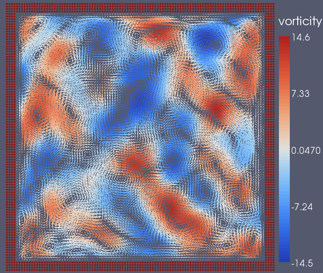
Figure 1: An typical initial velocity field for the decaying turbulence simulation. Arrows depict the velocity field and are coloured by the vorticity. The four layers of red dots around the edges of the box denote boundary SPH particles

In order to ensure a quiet start at the no-slip boundaries, the velocity field was gradually reduced down to zero near the boundaries by multiplying the velocity with a function $f(x)f(y)$ where

$$f(x)=1-\exp(-100(1-x^{2})^{2}).$$ (27)

The resultant velocity field is not necessarily divergence-free. However, the pseudo-spectral code described by Clercx et al. ensures that it is by projecting the velocity onto a divergence-free subspace. Following this example, we have performed a similar operation on velocity field defined by (25) - (27).

Any velocity field can be separated into its divergence-free component $\mathbf{v}_{d}$ and the gradient of a scalar $\phi$

$$\mathbf{v}=\mathbf{v}_{d}+\nabla\phi.$$ (28)

Taking the divergence of both sides gives

$$\nabla\cdot\mathbf{v}=\nabla^{2}\phi.$$ (29)

Since the SPH particles are initially on a grid, this equation can be solved for $\phi$ using a second order finite difference method. The divergence free velocity field $\mathbf{v}_{d}=\mathbf{v}-\nabla\phi$ is then normalised so that the total kinetic energy $E(0)=1$ per unit mass. Figure 1 shows an example of an initial velocity field generated using this method.

In order to be absolutely consistent, the pressure of the particles should be set to match the given velocity field. However, this was not expected to alter the results significantly as the SPH pressures quickly evolve to match the velocity field over a time scale set by the sound speed, which is 10 times greater than the maximum velocity of the flow.

5 Simulation Parameters

The Reynolds Number was set to $Re=\ell U/\nu=1500$ based on the half-width of the box $\ell=1$ and the initial RMS velocity $U=1$ of the particles. The simulation time $t$ is scaled by $\ell/U$ and is dimensionless. $t=1$ is comparable to one eddy turn-over time [25].

The particle densities and the reference density were set to $\rho=\rho_{0}=1000$. Therefore, the initial pressure field of the particles will be constant and equal to zero.

The simulated domain was a square box defined by $(-1\leq x,y\leq 1)$. The number of particles in the box was set to $300\times 300$ and the ratio between smoothing length and particle separation was $h/\Delta p=1.95$. Convergence studies (shown in Section 11) have indicated that the results of the decaying turbulence simulations are sufficiently converged using these resolution parameters.

6 Vorticity Evolution

The vorticity for each particle $a$ is determined as follows. A linear estimate of the velocity field around particle $a$ is defined as

$$v_{x}(x,y) =a_{1,1}(x-x_{a})+a_{1,2}(y-y_{a})$$ (30)

$$v_{y}(x,y) =a_{2,1}(x-x_{a})+a_{2,2}(y-y_{a}),$$ (31)

where $\mathbf{v}=(v_{x},v_{y})$ is the linear velocity estimate. The vorticity of particle $a$ is thus

$$\omega_{a}=\left(\nabla\times\mathbf{v}\right)_{a}=a_{2,1}-a_{1,2}.$$ (32)

In order to calculate the linear velocity coefficients, a least squares method was used to minimize the squared error between the actual SPH velocities of a set of particles in the neighbourhood of particle $a$ (i.e. within $2h$), and the linear estimate.

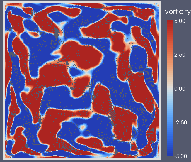
(a) $t=0$

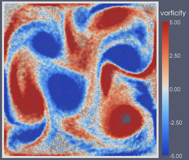
(b) $t=3.2$

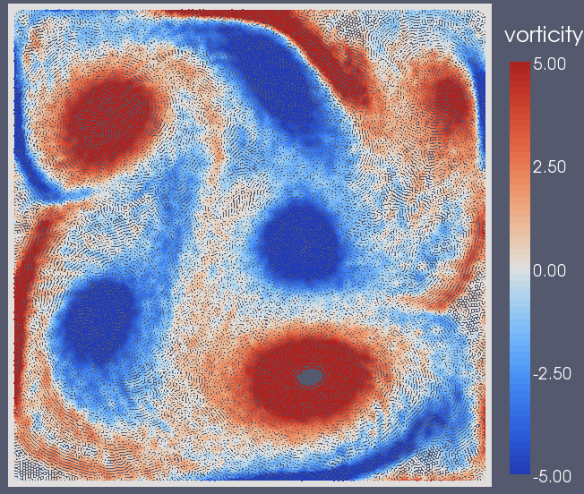
(c) $t=6.3$

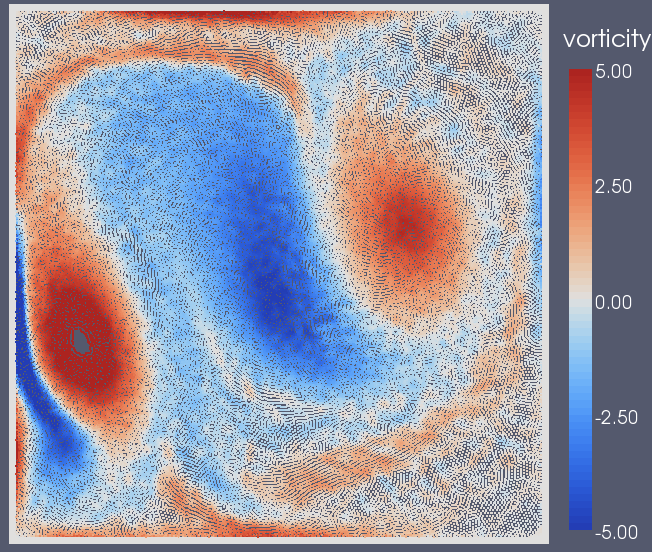
(d) $t=12.6$

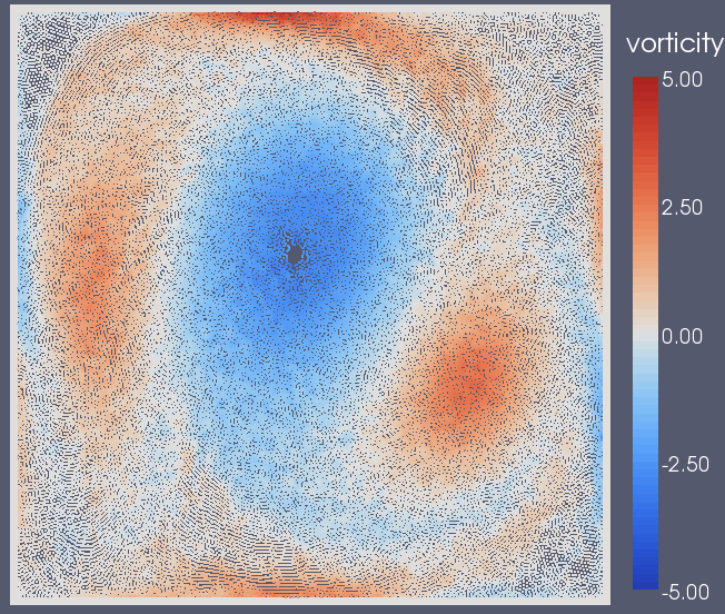
(e) $t=25.2$

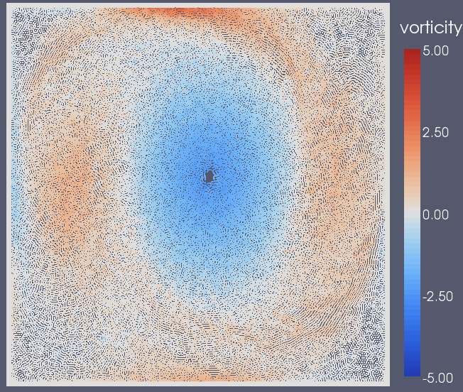
(f) $t=37.8$

Figure 2: Evolution of a typical decaying turbulence simulation, which shows the decay of the initial turbulent vorticity field to a single large vortex. The particles are coloured by vorticity, which has been clipped to $\pm 5$ in order to show the field at later times.

Figure 2 shows a number of snapshots from the simulation with the particles coloured by vorticity. The vorticity range has been clipped between $\pm 5$ in order to show the vortex structure at later times. Figure 2 shows the evolution of the vorticity field from the initial turbulent field to the final state, a single large vortex taking up most of the domain. Note that this is an example of the most likely evolution of the turbulence field, corresponding to a strong spin-up (i.e. increase in total angular momentum) of the fluid into a single large vortex. Clercx et al. [25] reported three main categories of evolution, the other two being a weak or delayed spin-up and no spin-up at all. This last case is characterised by having a final state consisting of a pair of vortices with opposite spin. See Section 7 for more details.

The initial evolution of the vorticity field occurs quite rapidly. Vortices usually either merge with neighbours with a similar rotation direction or are stretched out into thin vortex filaments (and ultimately erased through the action of viscosity) by vortices with an opposite spin. More rarely, a large vortex can be split by a counter-rotating vortex into two smaller but still coherent vortices. After $t\approx 20$ the flow has settled down enough so that there are only a few vortices left, and typically one monopole vortex that is comparable to the size of the domain. This monopole vortex is also the indicator of the spontaneous increase in total angular momentum for the flow, also known as the spontaneous spin-up. Subsequent to this, the other, smaller vortices gradually fade away until only the single, large vortex remains, along with the boundary layers that it excites along the surrounding walls.

Most of these snapshots show strong boundary layers being generated by vortex interactions with the walls. These are lifted away from the boundary to form vortex filaments. However, these are generally short-lived and do not persist as coherent vortices. Clercx et al. [25] reported that the vortex filaments contributed significantly to the turbulence over $1<t<20$. The filaments are generated at the boundary and move into the flow to become either elongated vorticity filaments or would be rolled up to form a coherent vortex. This vortex would often pair up with an existing vortex to form a dipole structure. In the SPH results only the first of these two options is seen. The vorticity filaments are produced at the boundary and lifted away to briefly form elongated filaments before they are erased by viscosity. Very occasionally the filament would roll up to become a roughly round vortex, however these structure were always much weaker than the surrounding structures and were always quickly dissipated.

7 Total Angular Momentum and Spontaneous Spin-Up

Figure 3 shows the normalised total angular momentum $\tilde{L}(t)=L(t)/L_{n}(t)$ for 12 randomly initialised simulations. The total angular momentum $L(t)$ is calculated around the centre of the box and is normalised by $L_{n}(t)$, the angular momentum of an equivalent mass of fluid with identical kinetic energy $E(t)$ moving in rigid body rotation (i.e. $L_{n}(t)=\sqrt{16\rho\ell^{4}E(t)/3}$). Of the 12 simulations, 8 of them show a rapid, spontaneous spin-up that was clearly established by $t\approx 20$. A further 2 simulations showed a slightly slower spin-up (solid red lines), and the final 2 simulations show little or no spin-up (thicker purple lines). This is identical to the ratio reported by Clercx et al. in their pseudo-spectral results. Out of 12 simulations, 8 showed a strong spin-up, 2 a weak spin-up and the final 2 showed no spin-up.

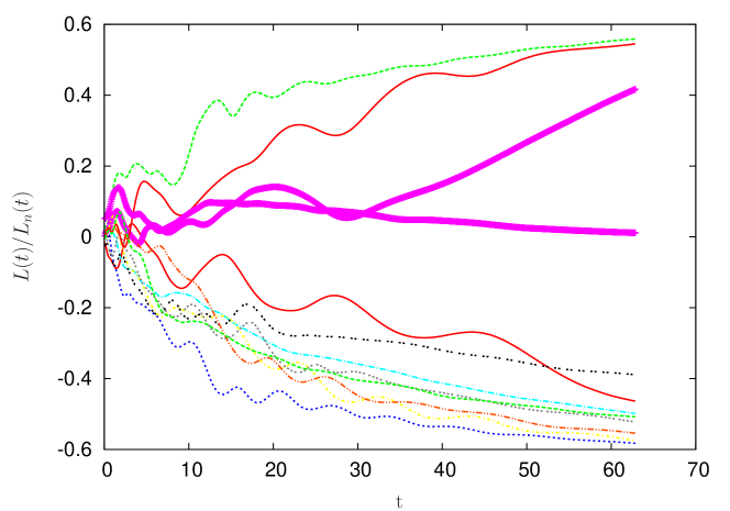
Figure 3: Each plot gives the total normalised angular momentum for each ensemble run. The normalised angular momentum is given by $L(t)/L_{n}(t)$, where $L_{n}(t)$ is the angular momentum of an equivalent mass of fluid with the same kinetic energy $E(t)$ moving in rigid body rotation. That is, $L_{n}(t)=\sqrt{16\rho\ell^{4}E(t)/3}$

This strong spin-up is the primary characteristic of turbulence in a square wall-bounded domain. Due to the geometry of the boundary, the pressure forces normal to the wall exert a net torque on the flow. The particular direction of this torque is highly dependant on the initial velocity field. We have used an initial field with an angular momentum close to zero and hence different random fields produce a spin-up in either direction. Other decaying turbulence experiments [35] have shown that simulations with a net initial angular momentum can still spin-up in either direction, although if the spin-up was in the opposite direction to the initial value then the strength of the final spin-up is reduced accordingly.

The normalised angular momentum plots given by Clercx et al. [25] indicate that the simulations with a strong spin-up will converge to an angular momentum of $|\tilde{L}|=0.6$. This is consistent with the SPH results.

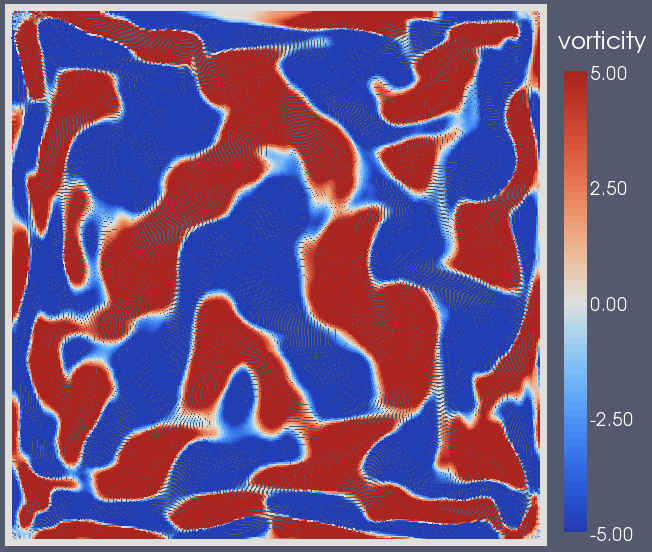
(a) $t=0$

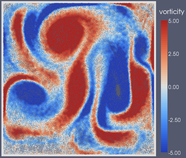
(b) $t=3.2$

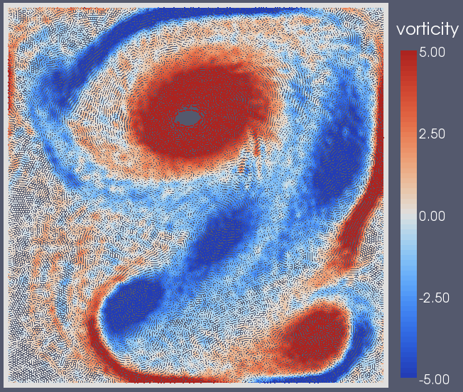
(c) $t=6.3$

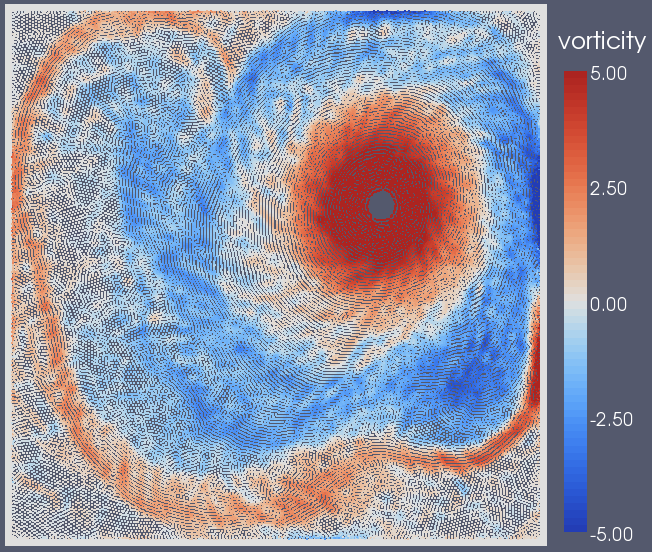
(d) $t=12.6$

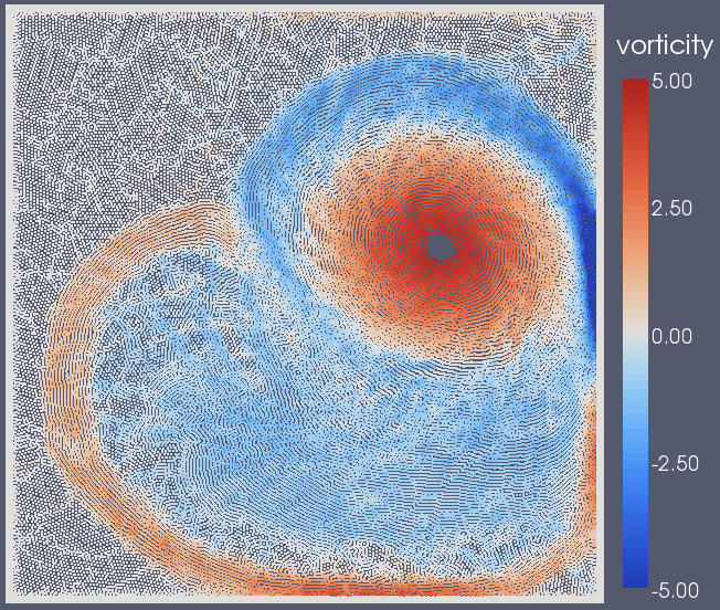
(e) $t=25.2$

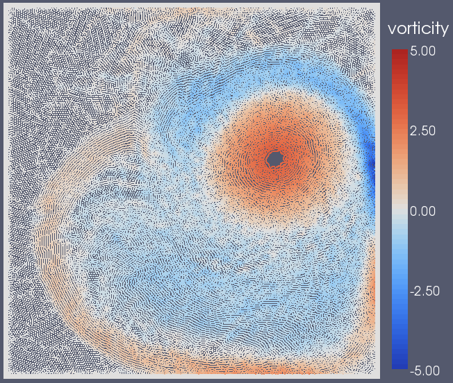
(f) $t=37.8$

Figure 4: Evolution of a decaying turbulence simulation that shows the rarer case where there is no spontaneous spin-up of the fluid.

Figure 4 shows the vorticity evolution for one of the SPH simulation that showed little or no spin-up. As is characteristic of these cases, instead of evolving into a single monopole vortex the initial turbulence instead decays to a dipole vortex structure. This is seen most clearly in the snapshot at $t=25.2$. There is still obviously a stronger vortex of the two, but the dipole structure persists long enough to only cause a weak spin-up. Looking back at the angular momentum plots in Figure 3, this vorticity evolution corresponds to the thick purple $\tilde{L}(t)$ plot that shows no spin-up until $t=30$ when $\tilde{L}(t)$ suddenly starts to increase. At this time the weaker vortex of the dipole dissipates, allowing the remaining vortex to induce the spontaneous spin-up.

8 Kinetic Energy Decay

Figure 5 shows the variation of total kinetic energy and enstrophy with time. These ensemble statistics were calculated by averaging over the 12 different simulation runs. They are both normalised by their values at $t=0$. That is, $\tilde{E}(t)=E(t)/E(0)$ and $\tilde{\Omega}(t)=\Omega(t)/\Omega(0)$.

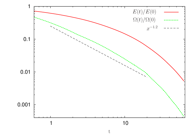
Figure 5: Ensemble average of total normalised kinetic energy and enstrophy for all 12 decaying turbulence simulations.

The decay of kinetic energy and enstrophy is rapid over the time period from $t=0$ to $t\approx 20$. During this time the flow is turbulent and there are many dissipative interactions between the vortices. Initially, the decay of enstrophy is significantly greater than the kinetic energy. This is expected from a two-dimensional turbulent flow, where the kinetic energy decay will approach zero as $Re\rightarrow\infty$. As the simulated turbulence decays, the Reynolds number of the flow decreases and the decay rate of the enstrophy and kinetic energy become comparable. After $t\approx 20$ the turbulence has evolved into a single monopole vortex (in most cases), and the kinetic energy and enstrophy decay level out to a roughly exponential decay.

The experimental results by Maassen et al. [36] show a power law decay for both kinetic energy and enstrophy for $1<t<20$. The kinetic energy decay shown in the SPH simulations does not follow this power law. However, Maassen et al. state that 3D stratification effects in their experiments had a large impact on the kinetic energy dissipation of the turbulence. The kinetic energy decay shown here is closer in form to the pseudo-spectral 2D turbulence simulations shown by Clercx et al. [25]. While Clercx et al. do not provide any curve fitting for their kinetic energy decay plots, they are qualitatively similar to the SPH results. In addition, both simulations have the same average decay rate over $0<t<60$. For $Re=1500$, their pseudo-spectral results showed a decay from $\tilde{E}=1$ to $\tilde{E}=0.001$ over approximately 60 time units. This is consistent with the SPH results.

The initial SPH enstrophy decay is similar to the power law seen in the experimental results by Maassen et al. [36]. Maassen et al. state that, with a weak stratification, the enstrophy decay over $1<t<20$ is proportional to $t^{\alpha}$, where $\alpha=-1.5\pm 0.2$. The decay of the SPH enstrophy over the same time period fits a power law with $\alpha=-1.2$. This is slightly less than the experimental results, however, Maassen et al. also show a slight decrease in $\alpha$ with decreasing stratification, indicating that 3D effects in the experiments act to increase the enstrophy dissipation. Therefore it can be concluded that the SPH enstrophy decay is consistent with these experimental results.

9 Average Wavenumber Decay

In Fourier or wavenumber space the total enstrophy $\Omega(t)$ is related to the kinetic energy spectrum by

$$\Omega(t)=\frac{\pi^{2}}{L^{2}M}\int_{0}^{\infty}k^{2}E(k)dk.$$ (33)

where $E(k)$ is the kinetic energy at the integer wavenumber $k$ (defined such that the wavelength of each mode is $\lambda=\frac{2L}{k}$) and $M$ is the total mass. It is reasonable to define an ”average” squared wavenumber $\langle k^{2}\rangle$ as [25]

$$\langle k^{2}\rangle=\frac{\Omega(t)}{E(t)}\sim\frac{\int_{0}^{\infty}k^{2}E(k)dk}{\int_{0}^{\infty}E(k)dk}$$ (34)

This variable is an indication of the average squared size of the eddies present in the turbulence. Taking an ensemble average of the average wavenumber over all 12 SPH simulations gives the plot shown in Figure 6. Also shown in this plot are two reference lines. Clercx et al. [25] found that the decay in $\langle k^{2}\rangle$ was approximately $t^{-0.63}$ from $t\approx 0.7$ to $t\approx 10$. This scaling is depicted by the lower, purple reference line. The decay in $\langle k^{2}\rangle$ for the SPH results is slightly less than this over the same time period, indicating that the evolution of the kinetic energy into larger vortex structures is slightly slower for the SPH simulations. In other words, the strength of the inverse energy cascade is weaker.

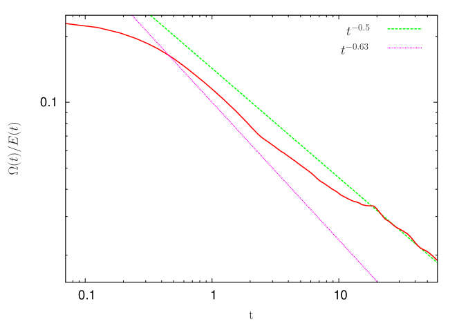
Figure 6: Ensemble average of $\Omega(t)/E(t)$, where $E(t)$ is the total kinetic energy and $\Omega(t)$ is the total enstrophy. This gives an estimate of the mean squared wavenumber $\langle k^{2}\rangle$. The higher dashed green reference line shows the average slope of the SPH results for $t>20$, the lower dashed violet reference line shows the scaling reported by Clercx et al. [25] over the time period $0.7<t<10$.

After $t=20$ the turbulence clearly enters a different evolutionary stage. Leading up to this time, over $10<t<20$, the decay in the average wavenumber begins to level off. At $t=20$ this trend is suddenly reversed and $\langle k^{2}\rangle$ resumes decaying. After this time a significant amount of fluctuation is introduced to the plot of $\langle k^{2}\rangle$. The rate of decay for $t>20$ is approximately $t^{-0.5}$, as shown by the higher, green reference line. Both the behaviour of the average wavenumber at $t=20$ and a similar rate of decay for $t>20$ is also seen in the pseudo-spectral results by Clercx et al.

This sudden change in $\langle k^{2}\rangle$ signals the formation of the large monopole vortex that is the typical end-state of these simulations. The interesting point to make about the dominant ”kink” in $\langle k^{2}\rangle$ is that it is not smoothed out due to the ensemble averaging over the 12 simulations. All these simulations have different initial velocity fields that lead to quite different evolutions for the turbulent flow. As we have already noted, the coherent vortices and hence the germination of the large monopole vortex is always embedded in this initial velocity field. It is therefore interesting that this vortex (or the dipole vortex in the case of no spin-up) is formed at the same time in each simulation, and its effects on the average wavenumber of the flow are so consistent across the ensemble simulations.

10 Kinetic Energy Spectrum

In the late sixties Batchelor [20] and Kraichnan [21] published their seminal papers on two-dimensional turbulence. They proposed the idea of an enstrophy cascade, in which the interactions between eddies resulted in a movement of enstrophy to increasingly higher wavenumbers. Using the assumption that the interactions of the turbulent eddies were local in wavenumber and that the kinetic energy spectrum is self-similar over time and space, they derived the following scaling law for the kinetic energy spectrum.

$$E(k)\sim\beta^{2/3}k^{-3}.$$ (35)

Due to the walls of the box, Batchelor and Kraichnan’s assumption of isotropic and homogeneous turbulence is no longer valid and therefore the classical $k^{-3}$ enstrophy cascade spectrum is not necessarily expected. However, numerical experiments of decaying turbulence (from an initial regular array of gaussian vortices) in a no-slip box [37] have provided some data for comparison. In this paper, Clercx and van Heijst compare the kinetic energy spectrum of periodic and wall-bounded turbulence, using a one dimensional spectrum obtained by a Chebyshev expansion of the kinetic energy and averaging over specific $x$ and $y$ coordinates to distinguish between the centre of the box and the neighbourhood of the no-slip walls. Near the no-slip boundaries, the authors show that there is an absence of a direct enstrophy cascade and that the kinetic energy spectrum is much flatter in the inertial range than the periodic case (the spectrum scales as $k^{-5/3}$ for $Re=20,000$ and $k^{-2.4}$ for $Re=5000$). Further away from the boundaries, they show that a $k^{-3}$ inertial range quickly forms near the centre of the box. However, in contrast to the periodic case, this spectrum flattens slightly over time, evolving to $k^{-2.1}$ for $Re=20,000$ or $k^{-2.5}$ for $Re=5000$.

In order to compare against the SPH results, a method is needed to perform a Fourier transform over the SPH particles. Since they will be unevenly distributed, traditional Fast Fourier Transform methods are of no use unless the particle variables are first interpolated to a grid, which would artificially reduce the spectrum at large wavenumbers.

Mansour [12] proposed a SPH Fourier transform by taking the usual form of the Fourier transform and simply replacing the integral with an SPH sum over all the particles. For example, a 2D Fourier transform over a periodic square of side $2L$ is

$$F(\mathbf{k}) =\frac{1}{L^{2}}\int_{-L}^{L}\int_{-L}^{L}f(\mathbf{r})e^{-i\frac{\pi}{L}\mathbf{k}\cdot\mathbf{r}}dxdy,$$ (36)

where $\mathbf{k}$ is an integer wavevector and $f(\mathbf{r})$ is the function being transformed. Converting this equation into an SPH summations, this becomes

$$F(\mathbf{k}) =\frac{1}{L^{2}}\sum_{b=1}^{N}f_{b}e^{-i\frac{\pi}{L}\mathbf{k}\cdot\mathbf{r}_{b}}\frac{m_{b}}{\rho_{b}},$$ (37)

where $\mathbf{r}_{b}$, $m_{b}$ and $\rho_{b}$ are the position, mass and density of particle $b$ and $f_{b}$ is the variable that is being transformed to the Fourier domain. The 2D spectrum $F(\mathbf{k})$ is then collapsed to a 1D spectrum by averaging over the angles in wavenumber space. That is

$$F(k)=\frac{1}{\sum_{k-1<|\mathbf{k}|\leq k}1}\sum_{k-1<|\mathbf{k}|\leq k}|F(\mathbf{k})|,$$ (38)

where $k=|\mathbf{k}|$.

Mansour [12] tested the accuracy of this SPH Fourier transform in 2D using a number of test spectra and density profiles and found that accurate results were obtained up to wavenumber $k_{c}=0.39N$, where $N$ is the number of particles along that dimension. Additional tests by the authors have shown that the transform is accurate up to wavenumber $k_{c}=0.26N$. Consequentially, all the spectra shown in this paper are shown over the range $0<k<0.26N$.

Due to the no-slip boundaries, the results will no longer satisfy the periodic assumption. Following the example of Wells et al. [38], the variable to be transformed is first reduced by its mean and then a Hann window is applied. Therefore, to calculate the kinetic energy spectra, the variable $f_{b}$ in (37) is calculated using

$$f_{b}=\begin{cases}0.5(1-cos(\pi(|\mathbf{r}_{b}|+1)))(\frac{1}{2}m_{b}\mathbf{v}_{b}\cdot\mathbf{v}_{b}-\frac{\sum_{a}{\frac{1}{2}m_{a}\mathbf{v}_{a}\cdot\mathbf{v}_{a}}}{N}),&\mbox{for }|\mathbf{r}_{b}|\leq 1,\\ 0,&\mbox{ otherwise}.\end{cases}$$ (39)

In order to determine the effect of the Hann window on the spectrum, a turbulent velocity field was taken from a previous DNS SPH simulation of forced turbulence in a periodic domain. In this case, the assumption of periodicity is valid and the kinetic energy spectrum can be calculated without the Hann window. The result is shown in Figure 7, along with the spectrum calculated after pre-multiplying by the Hann window.

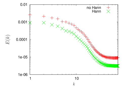
Figure 7: Kinetic energy spectrum calculated using the SPH Fourier transform of a periodic turbulent velocity field. This plot shows the effect of pre-multiplying the kinetic energy by a Hann window (Equation 39).

The original spectrum is shown using red plus symbols. The spectrum calculated by pre-multiplying by the Hann window is shown using green crosses, and is approximately one third of the original spectrum over all the wavenumbers calculated. Therefore, it can be concluded that the windowing does not significantly bias the shape of the spectrum, nor will it have any effect on the $k^{-3}$ enstrophy cascade scaling law.

Using this method for finding the SPH Fourier transform, the kinetic energy spectrum of the SPH results have been calculated at four different timesteps during the evolution of the decaying turbulence over $0<t<22$. This period covers the decay of the turbulence to the final domain-filling monopole or dipole vortex. Figure 8 shows the resultant spectra, which have been averaged over the 12 ensemble simulations.

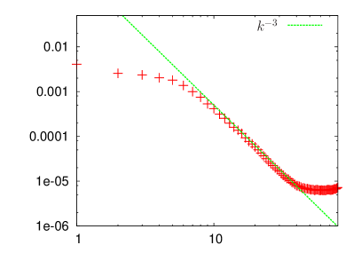
(a) $t=0.63$

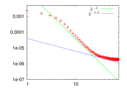
(b) $t=3.77$

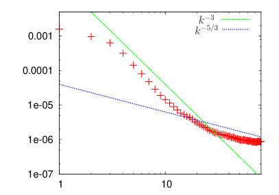
(c) $t=9.42$

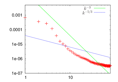
(d) $t=21.99$

Figure 8: Evolution of the kinetic energy spectrum $E(k)$ during the formation of the single monopole or dipole vortex. Each spectrum is plotted against the wavenumber $k$.

By $t=0.63$ the SPH simulation has established a clear $k^{-3}$ inertial range, which matches the published pseudo-spectral results by Clercx and van Heijst [37]. The $k^{-3}$ range occurs at wavenumbers $7<k<40$. The lower bound at $k=7$ is reasonable, and is an indication of the largest scale of the initial velocity field. The upper bound of $k=40$ is unexpected, as the inertial range (and the $k^{-3}$ scaling) should continue down to the dissipation length scale. This flattening of the spectrum is not seen in the pseudo-spectral simulations in [37]. Clercx and van Heijst do report that the spectrum flattens slightly over time at higher wavenumbers, but this process does not start before 2 vortex turn-over times (i.e. $t\approx 2$).

For $t>0.63$, the flattening of the spectrum spreads to smaller wavenumbers as the turbulence decays. The reference lines shown in plots (b)-(c) show a range of approximately $k^{-0.8}$ that grows to $k>20$ by $t=21.99$. While a similar flattening was reported in [37] for $t>4$, this effect was much more subtle. Instead of the $k^{-0.8}$ scaling seen in the SPH results (for $Re=1500$), Clercx and van Heijst [37] report that the spectrum flattens to $k^{-2.5}$ for $Re=5000$, and $k^{-2.1}$ for $Re=20,000$.

The results from the SPH kinetic energy spectrum are mixed. While the SPH results show a clear direct enstrophy cascade for much of the inertial range, as indicated by the $k^{-3}$ spectrum, the kinetic energy spectrum at high wavenumbers does not match the pseudo-spectral simulations of [37]. While this might be partially attributed to the differences in the simulations, in terms of initial velocity field and Reynolds number, of most concern is the deviation of the $k^{-3}$ spectrum shown at $t=0.63$. This is seen at very small times, when the majority of the fluid in the box has not interacted with the boundaries. At these times the kinetic energy spectrum should match the classical direct enstrophy cascade $k^{-3}$ that is predicted by 2D turbulence theory and normally seen in periodic 2D turbulence simulations.

However, it must be noted that the evolution of the integral variables of the SPH turbulence (e.g. total kinetic energy, enstrophy and angular momentum), do not seem to be significantly affected by the excess kinetic energy at high wavenumbers and correspond closely to the published pseudo-spectral results. This is an indication that this excess energy is largely cosmetic in nature and does not significantly affect the turbulence evolution, at least for the case of decaying turbulence.

11 Convergence Study

The numerical method SPH is based on both the integral interpolant (Equation 1) and the summation interpolant (Equation 2). The integral interpolant has a second order accuracy with the smoothing length $\mathcal{O}(h^{2})$. The accuracy of the summation interpolant is more complicated and depends on the distribution of the particles and hence the dynamics of the flow.

When performing a convergence study using SPH, it is important to vary both the number of particles used in the simulation, as well as the ratio of smoothing length to particle spacing $h/\Delta p$. Increasing the number of particles while keeping $h/\Delta p$ constant decreases the smoothing length $h$, which increases the accuracy of the integral interpolant while keeping the error due to the summation interpolant constant. Of course, if it is this latter error that is dominating the solution, increasing the number of particles while keeping $h/\Delta p$ fixed will have little effect on the solution.

Figure 9 shows the kinetic energy decay for a few different resolutions. The ratio of smoothing length to particle spacing $h/\Delta p$ is kept constant at 1.95 (all other SPH parameters, including the Reynolds number, are also kept constant). At the lowest resolution the accuracy of the simulation is poor and there is a substantial amount of numerical dissipation. As the resolution is increased, this dissipation is reduced and once the number of particles has increased beyond 300x300 there is no longer a significant change in the results, indicating that the solution (or at least this particular variable of the solution) has converged.

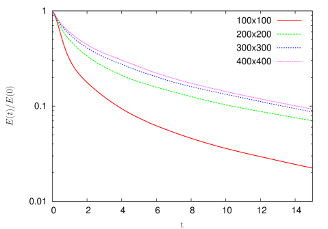
Figure 9: Decay of total normalised kinetic energy $\tilde{E}(t)$ from the same initial velocity field for different resolutions. $h/\Delta p$ is kept constant.

Figure 10 shows the same kinetic energy decay for increasing values of $h/\Delta p$. In each simulation the number of particles is also altered in order to keep $h$ constant at 0.013. This keeps the accuracy of the integral interpolant constant while varying the error for the summation interpolant. Using a value of $h/\Delta p\leq 1.3$, the long term decay of kinetic energy is significantly enhanced due to the excess dissipation caused by a noisy velocity field. However, setting $h/\Delta p\geq 1.4$ dramatically reduced this error and brought the results more into line with the pseudo-spectral kinetic energy decay rate.

For $h/\Delta p\geq 1.4$, the long term evolution of the total kinetic energy does not converge to a single decay rate. This is due to the chaotic nature of the decaying turbulence. While all the simulations have an identical initial velocity field, the variations in particle number and $h/\Delta p$ cause each simulation to evolve into a different flow. In a similar manner to the angular momentum results shown in Section 7, some simulations experience a strong spin-up while others only have a weak spin-up.

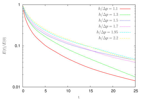
Figure 10: Decay of total normalised kinetic energy $\tilde{E}(t)$ from the same initial velocity field for different values of $h/\Delta p$. The smoothing length $h$ is kept constant.

12 Conclusion

The SPH results for decaying turbulence show a good agreement with all of the quantitative pseudo-spectral results from Clercx et al. [25]. The decay of kinetic energy and the characteristics of the spontaneous spin-up (i.e. it’s strength and likelihood) match well. The decay of the average squared wavenumber $\langle k^{2}\rangle$ is consistent with the pseudo-spectral results, although the decay rate over $0.7<t<20$ is slightly slower than that reported by Clercx et al. ($t^{-5}$ versus $t^{-0.63}$). However, the SPH results do reproduce the clear phase change in $\langle k^{2}\rangle$ at $t\approx 20$ which signals the formation of the final state for the turbulent decay.

The most significant differences between the two simulations are qualitative in nature. Clercx et al. [25] emphasised the importance that the boundaries play in injecting high intensity vorticity gradients into the flow. Clercx et al. showed that these vorticity filaments can roll up and persist for long times, travelling far into the interior of the flow as coherent vortices. This has been confirmed in both numerical experiment and experimental results. Wells et al. [38] have even set up a forced turbulence experiment where the flow was purely driven by the generation of vorticity filaments at the boundaries. In the SPH simulations strong boundary layers were generated at the boundaries in a similar manner to that described by Clercx et al. However, once these were lifted away from the wall they consistently failed to become long-lived structures. Instead, they were elongated into filaments that would either be destroyed by viscosity or merge with an interior vortex with an identical sign. None of the filaments rolled up to become coherent vortices. This problem is not due to the generation, and roll-up, of the boundary layers at the boundaries. Further results by the authors have shown that SPH can reproduce the correct boundary layer roll-up that is seen in experimental results [38]. Furthermore, Violeau and Issa [3] showed that SPH can produce accurate log-laws for the velocity of turbulence flow near a no-slip boundary. The problem occurs once these boundary layers are advected into the flow, where they are dissipated before they can interact with the flow to form long-term coherent vortices.

This paper has also examined the kinetic energy spectrum of the SPH decaying turbulence, using a Fourier transform that operates directly on the disordered particles. The spectrum shows the classical $k^{-3}$ spectrum that is expected from a direct enstrophy cascade. However, for high wavenumbers the spectrum unexpectedly flattens, indicating an excess of kinetic energy in the SPH results at small scales. The excess energy is initially seen length scales less than 7.5 particle spacings and grows in size as the turbulence decays.

However, the excess kinetic energy at small scales and the lack of the correct long-term evolution of these vorticity filaments seems to have little impact on the integral variables of the decaying turbulence (e.g. total kinetic energy, average squared wavenumber), all of which are reproduced satisfactorily by the SPH implementation. Future work in this area will focus on evaluating the performance of SPH at simulating continually forced turbulence. In this case, the dissipative characteristics of the method can be more easily evaluated by examining the energy balance between the power input via the forcing term, the viscous dissipation and the inverse energy cascade rate. The SPH DNS turbulence results will also be used as a baseline to compare with SPH turbulence models, most notably the consistent XSPH turbulence model proposed by Monaghan [39].

References

- [1] Cleary PW, Monaghan JJ. Boundary interactions and transition to turbulence for standard cfd problems using sph. Proc. 6th International Computational Techniques and Applications Conference, Canberra, 1993; 157–165.
- [2] Ting TS, Prakash M, Cleary PW, Thompson MC. Simulation of high reynolds number flow over a backward facing step using sph. Proceedings of the 7th Biennial Engineering Mathematics and Applications Conference, EMAC-2005, ANZIAM J., vol. 47, Stacey A, Blyth B, Shepherd J, Roberts AJ (eds.), 2006; C292–C309.
- [3] Violeau D, Issa R. Numerical modelling of complex turbulent free-surface flows with the SPH method: an overview. Int. J. Numer. Meth. Fluids 2007; 53:277–304.
- [4] Dalrymple R, Rogers B. Numerical modeling of water waves with the SPH method. Coastal Engineering Feb 2006; 53(2-3):141–147.
- [5] Shao S, Changming J, Graham D, Reeve D, James P, Chadwick A. Simulation of wave overtopping by an incompressible SPH model. Coastal Engineering 2006; 53:723–735.
- [6] Issa R, Violeau D, Laurence D. A first attempt to adapt 3d large eddy simulation to the smoothed particle hydrodynamics gridless method. Proceedings of the Int. Conf. Comput. and Experimental Eng. and Sciences, 1st Symposium on Meshless Methods, 2005.
- [7] Shao S, Gotah H. Simulating coupled motion of progressive wave and floating curtain wall by SPH-LES model. Coastal Engineering 2004; 46:171–202.
- [8] Violeau D, Piccon S, Chabard J. Two attempts of turbulence modelling in smoothed particle hydrodynamics. Proceedings of the 8th Symposium on Flow Modelling and Turbulence Measurements, Advances in Fluid Modelling and Turbulence Measurements, World Scientific: Singapore, 2002; 339–346.
- [9] Welton W. Two-Dimensional PDF/SPH Simulations of Compressible Turbulent Flows. Journal of Computational Physics Jan 1998; 139:410–443, 10.1006/jcph.1997.5878.
- [10] Monaghan JJ. SPH compressible turbulence. MNRAS 2002; 335:843–852.
- [11] Monaghan JJ. Energy transfer in a particle model. Journal of Turbulence 2004; 5:1–21.
- [12] Mansour JA. Sph and -sph: Applications and analysis. PhD Thesis, Monash University 2007.
- [13] Tran CV, Bowman JC. On the dual cascade in two-dimensional turbulence. Physica D: Nonlinear Phenomena 2003; 176(3-4):242 – 255, DOI: 10.1016/S0167-2789(02)00771-6. URL http://www.sciencedirect.com/science/article/B6TVK-47FDMHW-3/2/9a679ed3b1114fe4de7582f08a0d1ef3.
- [14] Davidson P. Turbulence: An introduction for scientists and engineers. Oxford University Press, 2004.
- [15] Lowe A. The direct numerical simulation of isotropic two-dimensional turbulence in a periodic square. PhD Thesis, University of Cambridge 2001.
- [16] Lilly DK. Numerical simulation of two-dimensional turbulence. Physics of Fluids 1969; 12(12):II–240–II–249, 10.1063/1.1692444. URL http://link.aip.org/link/?PFL/12/II-240/1.
- [17] Reynolds O. An Experimental Investigation of the Circumstances Which Determine Whether the Motion of Water Shall Be Direct or Sinuous, and of the Law of Resistance in Parallel Channels. [Abstract]. Royal Society of London Proceedings Series I 1883; 35:84–99.
- [18] Richardson LF. Atmospheric Diffusion Shown on a Distance-Neighbour Graph. Royal Society of London Proceedings Series A Apr 1926; 110:709–737.
- [19] Kolmogorov AN. Decay of isotropic turbulence in an incompressible viscous fluid. Dok. Akad. Nauk. SSSR 1941; 31:538.
- [20] Batchelor GK. Computation of the Energy Spectrum in Homogeneous Two-Dimensional Turbulence. Physics of Fluids Jan 1969; 12:233–+, 10.1063/1.1692443.
- [21] Kraichnan RH. Inertial Ranges in Two-Dimensional Turbulence. Physics of Fluids Jul 1967; 10:1417–1423, 10.1063/1.1762301.
- [22] Ayrton H. On a New Method of Driving off Poisonous Gases. Royal Society of London Proceedings Series A Oct 1919; 96:249–256.
- [23] Fujiwhara S. The natural tendency towards symmetry of motion and its application as a principle in meteorology. The Quarterly Journal of the Royal Meteorological Society Oct 1921; 47:287–292.
- [24] Smith LM, Yakhot V. Bose condensation and small-scale structure generation in a random force driven 2D turbulence. Physical Review Letters Jul 1993; 71:352–355, 10.1103/PhysRevLett.71.352.
- [25] Clercx HJH, Maassen SR, van Heijst GJF. Decaying two-dimensional turbulence in square containers with no-slip or stress-free boundaries. Physics of Fluids Mar 1999; 11:611–626, 10.1063/1.869933.
- [26] Li S, Montgomery D. Decaying two-dimensional turbulence with rigid walls. Physics Letters A Feb 1996; 218:281–291, 10.1016/0375-9601(96)00401-X.
- [27] Li S, Montgomery D, Jones WB. Two-Dimensional Turbulence with Rigid Circular Walls. Theoretical and Computational Fluid Dynamics 1997; 9:167–181, 10.1007/s001620050038.
- [28] Gingold RA, Monaghan JJ. Smoothed particle hydrodynamic: theory and application to non-spherical stars. Monthly Notices of the Royal Astronomical Society 1977; 181:375–389.
- [29] Lucy LB. A numerical approach to testing the fission hypothesis. The Astronomical Journal 1977; 82(12):1013–1924.
- [30] Monaghan JJ. Smoothed particle hydrodynamics. Reports of Progress in Physics Aug 2005; 68:1703–1759, 10.1088/0034-4885/68/8/R01.
- [31] Schoenberg IJ. Contributions to the problem of approximation of equidistant data by analytic functions, part a: On the problem of smoothing or gradu- ation, a first class of analytic approximation formulas. Quart. Appl. Math. 1946; 4(45).
- [32] Cole R. Underwater Explosions. Princeton University Press: Princeton, NJ, 1948.
- [33] Monaghan JJ. SPH and Riemann Solvers. Journal of Computational Physics Sep 1997; 136:298–307.
- [34] Hairer E, Lubich C, Wanner G. Geometric numerical integration illustrated by the stormer/verlet method. Acta Numerica 2003; :1–51.
- [35] van Heijst GJF, Clercx HJH, Molenaar D. The effects of solid boundaries on confined two-dimensional turbulence. Journal of Fluid Mechanics 2006; 554:411–431.
- [36] Maassen S, Clercx H, van Heijst G. Self-organization of quasi-two-dimensional turbulence in stratified fluids in square and circular containers. Physics of Fluids 2002; 14:2150.
- [37] Clercx H, van Heijst G. Energy spectra for decaying 2D turbulence in a bounded domain. Physical Review Letters 2000; 85(2):306–309.
- [38] Wells MG, Clercx HJH, van Heijst GJF. Vortices in oscillating spin-up. Journal of Fluid Mechanics 2007; 573:339–369, 10.1017/S0022112006003909.
- [39] Monaghan JJ. An sph turbulence model. Proc. 4th SPHERIC Workshop, 2009; 187–191.