Impact of surface imperfections on the Casimir force for lenses of centimeter-size curvature radii

Abstract

The impact of imperfections, which are always present on surfaces of lenses with centimeter-size curvature radii, on the Casimir force in the lens-plate geometry is investigated. It is shown that the commonly used formulation of the proximity force approximation is inapplicable for spherical lenses with surface imperfections, such as bubbles and pits. More general expressions for the Casimir force are derived that take surface imperfections into account. Using these expressions we show that surface imperfections can both increase and decrease the magnitude of the Casimir force up to a few tens of percent when compared with the case of a perfectly spherical lens. We demonstrate that the Casimir force between a perfectly spherical lens and a plate described by the Drude model can be made approximately equal to the force between a sphere with some surface imperfection and a plate described by the plasma model, and vice versa. In the case of a metallic sphere and semiconductor plate, approximately the same Casimir forces are obtained for four different descriptions of charge carriers in the semiconductor if appropriate surface imperfections on the lens surface are present. The conclusion is made that there is a fundamental problem in the interpretation of measurement data for the Casimir force, obtained by using spherical lenses of centimeter-size radii, and their comparison with theory.

I Introduction

The Casimir force 1 is caused by the existence of zero-point and thermal fluctuations of the quantized electromagnetic field. In the last few years physical phenomena grouped under the generic name of Casimir effect have received much experimental and theoretical attention 2 owing to numerous prospective applications in both fundamental and applied science. Many theoretical results in Casimir physics (for instance, on the role of skin depth or surface roughness) have already been experimentally confirmed (see Refs.17 ; 19 ; 9 ; 26 and review3 ). There is, however, one theoretical prediction made on the basis of the Lifshitz theory 2 ; 4 ; 5 which was unexpectedly found to be in contradiction with the experimental data. This is the large thermal effect in the Casimir force at short separations caused by the relaxation properties of free charge carriers in metals,6 semiconductors and dielectrics.7 ; 8 The respective experiments performed by means of micromechanical torsional oscillator,9 ; 10 ; 11 atomic force microscope 12 and Bose-Einstein condensate confined in a magnetic trap 13 ; 14 excluded the predicted effect at a high confidence level.

Almost all experiments on measuring the Casimir force between two macroscopic bodies were performed in the sphere-plate geometry.3 Experiments exploiting the sphere-plate geometry can be separated into experiments with small spheres of micrometer-size radii 17 ; 19 ; 9 ; 26 ; 10 ; 11 ; 12 ; 18 ; 20 ; 21 ; 22 ; 23 ; 24 ; 25 ; 27 ; 28 ; 29 and with large spherical lenses of centimeter-size curvature radii.30 ; 31 ; 29a ; 29aa In most of cases spherical surfaces were coated with Au (single exception is the experiment31 using a lens made of Ge). Small spheres (from a few tens to hundreds of micrometer radii) are usually made of polystyrene or sapphire. It is possible to control both global and local sphericity of small spheres microscopically by using, for instance, scanning electron microscopy. Large spherical lenses from a few centimeters to more than 10 cm curvature radii are made of glass or some other material. Allowed parameters of imperfections (defects) of their mechanically polished and ground surfaces are specified in the optical surface specification data provided by a producer (see, e.g., Refs.40 ; 41 ; 530a ).

It should be stressed that different defects are necessarily present on the surface of each (even of the best quality) optical lens.29b The reason is that when the glass is first made it may already contain defects such as bubbles. In grinding and polishing, a whole new set of surface defects such as scratches, digs, and chips may be introduced.29b In the subsequent technological operations of centering, beveling, cementing, and assembly, more defects are likely to be produced. The handling and operations involved in the numerous cleanings and inspections also add their quota of defects.29b Because of this, such a specification as “no bubbles or other imperfections permitted” is impossible to fulfil.29b Optical surface data specifying the parameters of defects permissible are obtained using scanning scattering microscopes, laser interference imaging profilometers and other techniques.29c The micrographs of different types of defects of optical surfaces taken with a differential interference contrast microscope can be found in Ref.29d . The scanning electron microscope images of defects are contained in Ref.29e . The most frequently present imperfections on lenses are digs, which include all hemispherical-appearing defects, and scratches whose length is usually much longer than the wavelength of the incident light.29b ; 29c ; 29d ; 29e ; 29f Note that in the large-scale applied problem of lens design29g surface inperfections play a rather limited role. However, as is shown below, they are very important for such a nonstandard application of lenses as for measurements of the Casimir force.

It is important to bear in mind that although large thermal corrections to the Casimir force at short separations were experimentally excluded, the thermal effect by itself in the configuration of two macrobodies has never been measured. In this respect experiments with lenses of large curvature radii attract much attention because they might allow measurements at separations of a few micrometers where predictions of alternative theoretical approaches (taking into account or discarding relaxation properties of free charge carriers) differ by up to 100%.

Experiments on measuring the Casimir force using spherical lenses of large radius of curvature have faced serious problems. The point is that calibration of the Casimir setup is usually performed by measuring electric forces between the sphere and plate from a potential difference applied to the test bodies (some nonzero residual potential difference exists even when the test bodies are grounded). Calibrations are performed by the comparison of the measured electric forces at different separations with the exact theoretical force-distance relation in the sphere-plate geometry, which is familiar from classical electrodynamics. Problems emerged when an anomalous force-distance relation for the electric force between an Au-coated spherical lens of $R=3.09\pm 0.015\,$cm curvature radius and a plate was observed,32 distinct from that predicted by classical electrodynamics (see also Ref.33 ). The existence of anomalous electrostatic forces was also confirmed in the configuration of Ge lens of $R=15.10\,$cm curvature radius and Ge plate,31 but denied 34 for an Au-coated small sphere of $R=100\,\mu$m radius interacting with an Au-coated plate.

It was shown 35 that the anomalous behavior of the electrostatic force can be explained due to deviations of the mechanically polished and ground surface from a perfect spherical shape for lenses with centimeter-size curvature radii. Different kinds of imperfections on such surfaces (bubbles, pits and scretches) can lead to significant deviations of the force-distance relation from the form predicted by classical electrodynamics under an assumption of perfectly spherical surface. Later this possibility was recognized 36 as a crucial point to be taken into account in future experiments not only in the sphere-plate geometry, but also for a cylindrical lens of centimeter-size radius of curvature near the plate.

In this paper we consider the possible imperfections on surfaces of lenses with centimeter-size radius of curvature, and calculate their impact on the Casimir force. The point to note is that the Casimir force is far more sensitive than the electrostatic force to the bubbles and pits that are always present on the mechanically polished and ground surfaces. The physical reason is that the Casimir force falls with the increase of separation distance more rapidly than the electric force. As a result, the Casimir force is determined by smaller regions near the points of closest approach of the two surfaces. If the local radius of curvature on the lens surface near the point of closest approach to the plate is significantly different from the mean radius of curvature $R$, the impact of such surface imperfection on the Casimir force can be tremendous.

We show that the presence of bubbles and pits on a lens surface, allowed by the optical surface specification data, makes inapplicable the simplified formulation of the proximity force approximation (PFA) used 30 ; 31 ; 29a for the comparison between experiment and theory. We also derive the expressions for the Casimir force applicable in the presence of bubbles and pits on surfaces of centimeter-size lenses. It is shown that for ideal metal bodies surface imperfections may lead to both a decrease and an increase in the magnitude of the Casimir force up to a few tens of percent for sphere-plate separations from 1 to $3\,\mu$m.

As discussed above, one might expect that experiments with large lenses will help to resolve the problem with the thermal Casimir force. In this connection we consider real metal spherical lens, with surface imperfections of different types, close to a real metal plate both described either by the Drude dielectric function (relaxation of free charge carriers is included) or by the dielectric function of the plasma model where the relaxation parameter of free charge carriers is set to zero. We show, that the Casimir force between a perfectly spherical lens and a plate, both described by the Drude model, in the limit of experimental error, is equal to the Casimir force between a lens with some specific surface imperfection and a plate, both described by the plasma model. Vice versa, we demonstrate that if the metal surface of the perfectly shaped lens and a plate is described by the plasma model, this can lead to approximately the same Casimir force over the separation region from 1 to $3\,\mu$m as for a lens with some imperfection and a plate, both described by the Drude model. It has been known that experimentally it is hard to determine the position of the point of closest approach between a lens and a plate on the lens surface with sufficient precision. Then it remains uncertain what kind of surface imperfection (if any) is located near the point of the closest approach. This leads us to the conclusion that experiments with large spherical lenses are in fact unsuitable for resolving the problem of the thermal Casimir force between real metals.

Results similar in spirit are obtained for an Au-coated lens of centimeter-size radius of curvature interacting with a semiconductor or dielectric plate. We calculate the Casimir force between a perfectly spherical Au-coated lens and a dielectric (high-resistivity Si) plate with the neglect of free charge carriers (in so doing it makes almost no difference whether the Drude or the plasma model is used for the description of Au). We show then that approximately the same Casimir force over the separation region from 1 to $3\,\mu$m is obtained for an Au sphere with appropriately chosen surface imperfections and the following models of a semiconductor plate: 1) High-resistivity Si with included dc conductivity; 2) Low-resistivity Si with charge carriers described by the Drude model; 3) Low-resistivity Si with charge carriers described by the plasma model. Here, free charge carriers of the Au sphere are described by the Drude model in cases 1) and 2), and by the plasma model in the case 3). Thus, experiments with large spherical lenses are also not helpful for resolving the problem of dc conductivity of semiconductor or dielectric materials in the Lifshitz theory.

The structure of the paper is as follows. In Sec. II we consider spherical lenses with surface imperfections of different types and derive the formulations of the PFA applicable for deformed spherical surfaces. Demonstration of the influence of surface inperfections on the magnitude of the Casimir force in the simplest case of ideal metal bodies is contained in Sec. III. Section IV is devoted to the calculation of the Casimir force between a real metal plate and a real metal lens with surface imperfections. In Sec. V similar results are presented for a real metal lens interacting with a semiconductor or dielectric plate. Our conclusions and discussions are contained in Sec. VI.

II Proximity force approximation for spherical lenses with surface imperfections of different types

As discussed in Sec. I, the Casimir force should be more sensitive than the electrostatic force to surface imperfections that are invariably present on the mechanically polished and ground surfaces of any lens of centimeter-size curvature radius. However, in experiments on measuring the Casimir force in the lens-plate geometry, comparison between the measurement data and theory is usually performed by means of the simplified formulation of the PFA assuming perfect sphericity of the lens surface.2 ; 3 ; 37 We demonstrate first how this simplified formulation of the PFA is obtained from the most general formulation.38 Then we apply the general formulation of the PFA to lenses with surface imperfections of different types.

The most general formulation of the PFA represents the Casimir force between a lens surface $z=z(x,y)$ and a plate $z=0$ as an integral of the Casimir pressures between pairs of plane surface elements spaced at separations $z=z(x,y)$:

$$F_{sp}(a,T)=\int_{\Sigma}d\sigma P(z,T).$$ (1)

Here, $d\sigma$ is the element of plate area, $\Sigma$ is the projection of the lens onto the plate, $a$ is the shortest separation between them, and $P(z,T)$ is the pressure for two plane parallel plates at a separation $z=z(x,y)$ at temperature $T$.

We choose the origin of a cylindrical coordinate system on the plane $z=0$ under the lens center. Then for a perfectly shaped spherical lens of radius of curvature $R$ the coordinate $z$ of any point of its surface is given by

$$z=R+a-(R^{2}-\rho^{2})^{1/2},\quad\rho^{2}=x^{2}+y^{2}.$$ (2)

In this case Eq. (1) leads to

$$F_{sp}^{\rm perf}(a,T)=2\pi\int_{0}^{\sqrt{2RD-D^{2}}}\!\!\!\rho d\rho P(z,T)$$

$$~{}~{}~{}~{}~{}~{}~{}~{}~{}=2\pi\int_{a}^{D+a}(R+a-z)P(z,T)dz.$$ (3)

Keeping in mind that the Casimir pressure is expressed as

$$P(z,T)=-\frac{\partial{\cal F}_{pp}(z,T)}{\partial z},$$ (4)

where ${\cal F}_{pp}(z,T)$ is the free energy per unit area of parallel plates, and integrating by parts in Eq. (3), one arrives at

$$F_{sp}^{\rm perf}(a,T)=2\pi R{\cal F}_{pp}(a,T)$$

$$~{}~{}~{}-2\pi(R-D){\cal F}_{pp}(D+a,T)-2\pi\int_{a}^{D+a}\!\!{\cal F}_{pp}(z,T)dz.$$ (5)

We consider centimeter-size spherical lenses satisfying conditions $a\ll D$, $a\ll R$. For such lenses ${\cal F}_{pp}(D+a,T)\ll{\cal F}_{pp}(a,T)$. Because of this, one can neglect the second term on the right-hand side of Eq. (5) in comparison with the first.37 It can be also shown 37 ; 39 that the first term on the right-hand side of Eq. (5) is larger than the third by a factor of $R/a$. This allows one to neglect the third term and arrive to what is called the simplified formulation 37 ; 39 of the PFA

$$F_{sp}^{\rm perf}(a,T)\approx 2\pi R{\cal F}_{pp}(a,T)$$ (6)

widely used for both spherical lenses and for spheres [note that for a semisphere the second term on the right-hand side of Eq. (5) is exactly equal to zero].

The above derivation shows that the PFA in the form of Eq. (6) is applicable only at $a/R\ll 1$. For the real metal sphere (spherical lens) above real metal plate the analytic expressions for the Casimir force in terms of scattering amplitudes are available,37a ; 37b ; 37c but due to computational difficulties numerical results were obtained only under the condition37a ; 37b $a/R\geq 0.1$ and under the condition37c $a/R\geq 0.053$. Computations were performed for metals described by simple plasma and Drude models37a ; 37b and by the generalized plasma and Drude models taking into account interband transitions of core electrons.37c The relative deviations between the obtained exact results for the Casimir force and the approximate results calculated using the PFA in Eq. (6) were found to be less than $a/R$. It was demonstrated39 also that the PFA results approach the respective exact results with decreasing $a/R$. Keeping in mind that for the experiments performed to date with small spheres $a/R\approx 10^{-3}=0.1$% and for experiments with large spherical lenses $a/R\approx 10^{-5}=0.001$%, the use of the PFA for the comparison between experiment and theory is well justified.

Now we consider real lenses with centimeter-size radii of curvature. Surfaces of such lenses are far from perfect, even excluding the rms roughness of a few nanometers from consideration. In optical technology quality of lens surfaces is characterized 29b ; 29c ; 29d ; 29e ; 29f ; 29g ; 40 ; 41 in terms of scratch and dig optical surface specification data. In particular, depending on the quality of the lens used, digs (i.e., bubbles and pits) with a diameter varying 29b ; 40 from $30\,\mu$m to 1.2 mm are allowed on the surface. There may also be scratches on the surface with a width varying 29b ; 40 from 3 to $120\,\mu$m. The problem of bubbles on the centimeter-size lens surface should not be reduced to the fact that lens curvature radius $R$ is determined with some error. The thickness of each bubble or pit should of course be less than the absolute error in the measurement of lens radius of curvature (for a lens 31 with $R=15.10\,$cm, for instance, $\Delta R=0.05\,$cm). The crucial point is that curvature radii of bubbles and pits can be significantly different, as compared to $R$. Surface imperfections with these local radii of curvature, as we show below, can give a major contribution to the Casimir force.

As the first example we consider the lens with the curvature radius $R=15\,$cm having a bubble of the radius of curvature $R_{1}=25\,$cm and thickness $D_{1}=0.5\,\mu$m near the point of the closest approach to the plate [see Fig. 1(a)]. The radius of the bubble is determined from $r^{2}=2R_{1}D_{1}-D_{1}^{2}\approx 0.25\,\mbox{mm}^{2}$, leading to $2r=1\,\mbox{mm}<1.2\,$mm, i.e., less than a maximum value allowed 40 by the optical surface specification data. The respective quantity $d$ defined in Fig. 1(a) is equal to $d\approx r^{2}/(2R)\approx 0.83\,\mu$m. Then the flattening of a lens surface at the point of closest approach to the plate is $d-D_{1}\approx 0.33\,\mu$m which is much less than $\Delta R$.

The general formulation of the PFA (1) should be applied taking into account that the surface of the bubble is described by the equation

$$z=R_{1}+a-(R_{1}^{2}-\rho^{2})^{1/2},$$ (7)

where $a$ is the distance between the bottom point of the bubble and the plate [see Fig. 1(a)]. In this notation the surface of the lens is described by the equation

$$z=R+D_{1}-d+a-(R^{2}-\rho^{2})^{1/2}.$$ (8)

Using Eqs. (7) and (8) one arrives, instead of Eq. (3), at

$$F_{sp}(a,T) = 2\pi\int_{a+D_{1}}^{a+D_{1}-d+D}\!\!\!(R-z+D_{1}-d+a)P(z,T)dz$$ (9)

$$+2\pi\int_{a}^{a+D_{1}}(R_{1}-z+a)P(z,T)dz.$$

Now we take into consideration that the quantities $a$, $d$, and $D_{1}$ are smaller than the error in the determination of large radii $R$ and $R_{1}$. Then one can rearrange Eq. (9) to the form

$$F_{sp}(a,T)\approx 2\pi\int_{a+D_{1}}^{a+D_{1}-d+D}\!\!\!(R-z)P(z,T)dz$$

$$~{}~{}~{}~{}~{}~{}+2\pi R_{1}\int_{a}^{a+D_{1}}P(z,T)dz.$$ (10)

Here, the first integral on the right-hand side is calculated similar to Eqs. (3) and (5) leading to $2\pi R{\cal F}_{pp}(a+D_{1},T)$. Calculating the second integral with the help of Eq. (4), one finally obtains

$$F_{sp}(a,T)\approx 2\pi(R-R_{1}){\cal F}_{pp}(a+D_{1},T)+2\pi R_{1}{\cal F}_{pp}(a,T).$$ (11)

Now we consider two more examples of surface imperfection, specifically, a bubble with the curvature radius $R_{1}=5\,$cm [see Fig. 1(b)] and a pit with the curvature radius $R_{1}=12\,$cm [see Fig. 1(c)]. In both cases the curvature radius of the lens remains the same $R=15\,$cm. For the bubble we choose $D_{1}=1\,\mu$m which results in $r\approx 0.32\,$mm, $d\approx 0.33\,\mu$m, and $D_{1}-d\approx 0.67\,\mu$m in agreement with allowed values. Equation (11) is evidently preserved with the new values of parameters.

Now we deal with the pit shown in Fig. 1(c). Here, the lens surface near the point of closest approach to the plate is concave up, i.e., in the direction of the lens center. The related parameters are $D_{1}=1\,\mu$m, $r\approx 0.49\,$mm, $d\approx 0.8\,\mu$m, and $d+D_{1}\approx 1.8\,\mu$m. The pit surface is described by the equation

$$z=a+D_{1}-R_{1}+(R_{1}^{2}-\rho^{2})^{1/2}.$$ (12)

Here, $a$ is the separation distance between the plate and the points of the circle on the lens surface closest to it. The surface of the lens is described as

$$z=R+a-d-(R^{2}-\rho^{2})^{1/2}.$$ (13)

Repeating calculations that have led to Eq. (11) with the help of Eqs. (12) and (13), we obtain

$$F_{sp}(a,T)\approx 2\pi(R-R_{1}){\cal F}_{pp}(a,T)+2\pi R_{1}{\cal F}_{pp}(a+D_{1},T).$$ (14)

It is evident that Eqs. (11) and (14) lead to significantly different results than the simplified formulation of the PFA in Eq. (6). The reason is that at separations $a\gtrsim 1\,\mu$m we get $D_{1}\lesssim a$ and all three contributions on the right-hand side of Eqs. (11) and (14) are of the same order of magnitude. This is confirmed by the results of numerical computations for both ideal metals (Sec. III) and for real materials (Secs. IV and V).

III Demonstration of the role of surface imperfections for ideal metal bodies

We begin with the case of an ideal metal lens with surface imperfections shown in Fig. 1(a,b,c) near the point of closest approach to an ideal metal plate. The case of ideal metal bodies, although it disregards real material properties, allows the demonstration of the entirely geometrical effect of surface imperfections on the Casimir force.

To perform numerical computations by Eqs. (11) and (14) one needs convenient representation for the Casimir free energy per unit area, ${\cal F}_{pp}(z,T)$, in the configuration of two parallel ideal metal plates. The standard expression for this quantity is given by 2 ; 42

$${\cal F}_{pp}(z,T)=\frac{k_{B}T}{\pi}\sum_{l=0}^{\infty}{\vphantom{\sum}}^{\!\prime}\int_{0}^{\infty}k_{\bot}dk_{\bot}\ln(1-e^{-2zq_{l}}).$$ (15)

Here, $k_{B}$ is the Boltzmann constant, $k_{\bot}$ is the magnitude of the projection of the wave vector on the plates, $q_{l}^{2}=k_{\bot}^{2}+\xi_{l}^{2}/c^{2}$, $\xi_{l}=2\pi k_{B}Tl/\hbar$ with $l=0,\,1,\,2,\,\ldots$ are the Matsubara frequencies, and the primed summation sign means that the term with $l=0$ is multiplied by 1/2. The most frequently used form of Eq. (15) separates it into the contribution of zero temperature and thermal correction. For our purpose, however, it is more convenient to present Eq. (15) as a sum of the high-temperature contribution to the free energy and the correction to it. For this purpose we rewrite Eq. (15) in terms of a dimensionless integration variable $y=2aq_{l}$ and expand the logarithm in a power series

$${\cal F}_{pp}(z,T)=-\frac{k_{B}T}{4\pi z^{2}}\sum_{l=0}^{\infty}{\vphantom{\sum}}^{\!\prime}\int_{\tau_{z}l}^{\infty}ydy\sum_{n=1}^{\infty}\frac{e^{-ny}}{n}.$$ (16)

Here, the dimensionless parameter $\tau_{z}$ is defined as $\tau_{z}=4\pi zk_{B}T/(\hbar c)$. After performing integration and then the summation with respect to $l$, the following result is obtained:

$${\cal F}_{pp}(z,T)=-\frac{k_{B}T}{4\pi z^{2}}\left[\vphantom{\sum_{n=1}^{\infty}}\frac{\zeta(3)}{2}\right.$$ (17)

$$~{}~{}~{}~{}~{}~{}~{}~{}~{}+\left.\sum_{n=1}^{\infty}\frac{e^{-\tau_{z}n}}{n^{2}(1-e^{-\tau_{z}n})}\left(\frac{1}{n}+\frac{\tau_{z}}{1-e^{-\tau_{z}n}}\right)\right],$$

where $\zeta(x)$ is the Riemann zeta function. Note that the first contribution on the right-hand side of Eq. (17) is just the high temperature limit of the free energy. This is seen if we take into account that $\tau_{z}=2\pi T/T_{\rm eff}$, where the effective temperature is defined from $k_{B}T_{\rm eff}=\hbar c/(2z)$, and, thus, $\tau_{z}\to\infty$ when $T\gg T_{\rm eff}$.

Now we are in a position to compute the Casimir force between the spherical lens of large curvature radius with bubbles and pits of different types and a plane plate, both made of ideal metal. In the literature it is common to use the simplified formulation of the PFA (6) in the sphere-plate geometry for both small spheres of about $100\,\mu$m radii and large spherical lenses. 2 ; 17 ; 19 ; 9 ; 26 ; 3 ; 10 ; 11 ; 12 ; 18 ; 20 ; 21 ; 22 ; 23 ; 24 ; 25 ; 27 ; 28 ; 29 ; 30 ; 31 ; 29a ; 32 ; 33 ; 34 In doing so the role of bubbles and pits on the surface of lenses of centimeter-size curvature radii is neglected. Equation (6), however, is not applicable for lenses with large radius of curvature because it assumes perfect spherical surface. For such lenses one should use more complicated results like those in Eqs. (11) and (14). To illustrate this fact, we perform calculations for three typical model imperfections on the spherical surface near the point of closest approach to the plate shown in Fig. 1(a,b,c).

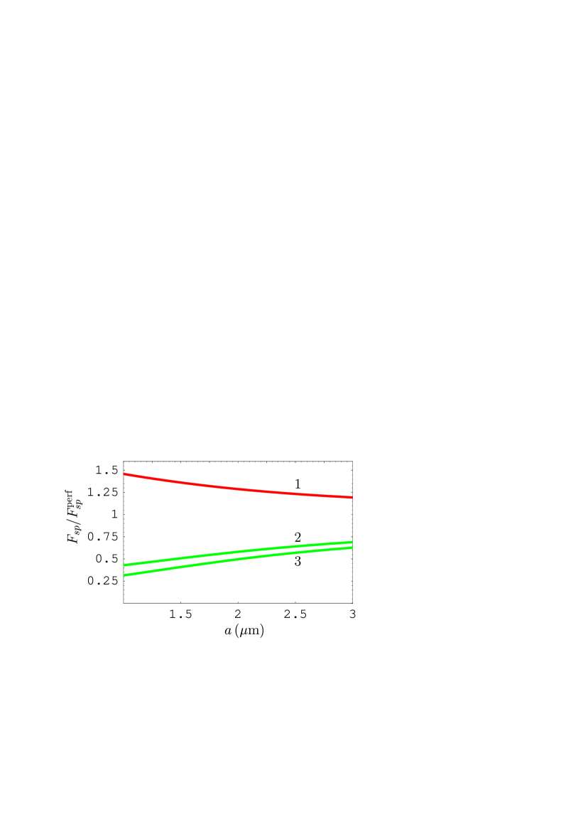
Figure 2: (Color online) The normalized Casimir force acting between an ideal metal spherical lens with surface imperfections of different types and an ideal metal plate as a function of separation. Lines 1, 2, and 3 are for the surface imperfections shown in Fig. 1(a,b,c), respectively.

We begin with the surface imperfection shown in Fig. 1(a), where the bottom of the spherical lens is flattened for approximately $0.33\,\mu$m (see Sec. II). Computations of the Casimir force $F_{sp}(a,T)$ in Eq. (11), taking the bubble into account, and the force $F_{sp}^{\rm perf}(a,T)$ in Eq. (6) for a lens with perfectly spherical surface were performed at $T=300\,$K with the help of Eq. (17) over the separation region from 1 to $3\,\mu$m. Computations at larger separations would be not warranted because the experimental error quickly increases with the increase of $a$. Thus, in the most well known measurement30 of the Casimir force by using large lens the relative error at $a=3\,\mu$m was shown40a to be larger than 47%. In the experiment31 with Ge test bodies the relative error in the measured Casimir force exceeds 100% at $a\geq 2\,\mu$m due to the error in subtracted residual electrostatic forces. The computational results for the ratio $F_{sp}(a,T)/F_{sp}^{\rm perf}(a,T)$ as a function of separation are presented in Fig. 2 by the line labeled 1. As can be seen in Fig. 2, in the presence of the bubble shown in Fig. 1(a), the use of Eq. (6) for perfect spherical surface instead of Eq. (11) considerably underestimates the magnitude of the Casimir force. Thus, at separations $a=1.0$, 1.5, 2.0, 2.5, and $3.0\,\mu$m the quantity $F_{sp}/F_{sp}^{\rm perf}$ is equal to 1.458, 1.361, 1.287, 1.233, and 1.193, respectively, i.e., the underestimation varies from 46% at $a=1\,\mu$m to 19% at $a=3\,\mu$m.

We continue with surface imperfection shown in Fig. 1(b), where the thickness of an extra bulge on the spherical lens around its bottom point is approximately equal to $0.67\,\mu$m (see Sec. II). Computations were performed with Eqs. (6) and (11) using Eq. (17). The computed values of the quantity $F_{sp}(a,T)/F_{sp}^{\rm perf}(a,T)$ as a function of separation are shown by the line labeled 2 in Fig. 2. It can be seen that in this case the assumption of perfect sphericity of a lens surface considerably overestimates the magnitude of the Casimir force. Thus, at separations $a=1.0$, 1.5, 2.0, 2.5, and $3.0\,\mu$m the values of the quantity $F_{sp}/F_{sp}^{\rm perf}$ are equal to 0.429, 0.507, 0.580, 0.641, and 0.689, respectively, i.e., overestimation varies from 57% at $a=1\,\mu$m to 36% at $a=3\,\mu$m.

Finally we consider the surface imperfection in the form of a pit presented in Fig. 1(c). Here, the deformation of the lens surface is characterized by the parameter $d+D_{1}\approx 1.8\,\mu$m. The computational results using Eqs. (6), (14) and (17) are shown by the line labeled 3 in Fig. 2. Once again, the assumption of perfect lens sphericity significantly overestimates the magnitude of the Casimir force. Thus, at separations $a=1.0$, 1.5, 2.0, 2.5, and $3.0\,\mu$m the ratio $F_{sp}/F_{sp}^{\rm perf}$ is equal to 0.314, 0.409, 0.496, 0.570, and 0.627, respectively, i.e., overestimation varies from 69% at $a=1\,\mu$m to 37% at $a=3\,\mu$m.

Thus, for an ideal metal lens above an ideal metal plate the use of the PFA in its simplest form (6) can lead to the Casimir force, either underestimated or overestimated by many tens of percent, depending on the character of imperfection on the lens surface near the point of closest approach to the plate. Below we show that for a lens with a centimeter-size radius of curvature and a plate made of real materials the role of imperfections of the lens surface increases in importance.

IV Test bodies made of real metal

At separations above $1\,\mu$m the characteristic frequencies giving major contribution to the Casimir force are sufficiently small. Because of this, one can neglect the contribution of interband transitions and describe the metal of the test bodies by means of simple Drude model. This leads to the dielectric permittivity depending on the frequency

$$\varepsilon_{D}(\omega)=1-\frac{\omega_{p}^{2}}{\omega(\omega+i\gamma)},$$ (18)

where $\omega_{p}$ is the plasma frequency and $\gamma$ is the relaxation parameter.

The dielectric permittivity (18) takes into account relaxation properties of free electrons by means of the temperature-dependent relaxation parameter $\gamma=\gamma(T)$. It is common knowledge that in the local approximation it correctly describes the interaction of a metal with the real (classical) electromagnetic field, specifically, in the quasistatic limit 43 where $\omega\to 0$. The behavior of $\varepsilon$ as the reciprocal of the frequency in this limit is the direct consequence41a of the classical Maxwell equations. It can be said that the Drude dielectric permittivity (18) is fully justified on the basis of fundamental physical theory and confirmed in numerous technical applications. The Drude model (18) also provides the correct description of out of thermal equilibrium physical phenomena determined by the fluctuating electromagnetic field such as radiative heat transfer and near-field friction.41b Because of this, a disagreement of Eq. (18) with the experimental data would be a problem of serious concern. However, as was noticed in Sec. I, precise experiments on measuring the Casimir pressure at separations below $1\,\mu$m by means of the micromechanical torsional oscillator 9 ; 10 ; 11 exclude large thermal effect in the Casimir force caused by the relaxation properties of charge carriers in metals. The results of these experiments are consistent with the plasma model

$$\varepsilon_{p}(\omega)=1-\frac{\omega_{p}^{2}}{\omega^{2}},$$ (19)

obtained from Eq. (18) by setting $\gamma=0$.

In classical electrodynamics43 ; 41a the plasma model is considered as an approximation valid in the region of sufficiently high infrared frequencies, where the electric current is pure imaginary and the relaxation properties do not play any role. In real (classical) electromagnetic fields the dielectric permittivity (19) does not describe the reaction of a metal on the field in the limit of quasistatic frequencies. As was noted above, Maxwell equations lead to $\varepsilon\sim 1/\omega$ in the limiting case $\omega\to 0$. The contradiction between the Lifshitz theory combined with the Drude model and the experimental data was widely discussed in the literature, 2 ; 3 ; 44 ; 45 ; 46 ; 47 ; 48 ; 49 ; 50 ; 51 ; 52 but a resolution has not yet been achieved. It was also suggested 53 that there might be some differences in the reaction of a physical system in thermal equilibrium with an environment to real fields with nonzero mean value and fluctuating fields whose mean value is equal to zero. Because of this, the possibility of measuring the thermal Casimir force at separations of a few micrometers, where the predicted results from using Eqs. (18) and (19) differ up to a factor of two, is of crucial importance.

We first consider surface inperfections introduced in Fig. 1(a,b,c) in Sec. II and compute their impact on the Casimir force between a lens and a plate, both described either by the Drude or by the plasma model. In so doing Eq. (11) remains valid for the imperfections of Fig. 1(a,b) and Eq. (14) for the imperfection of Fig. 1(c). As to the free energy per unit area of two parallel plates, one should use the following Lifshitz formula 2 ; 3 ; 4 ; 5 instead of Eq. (17):

$${\cal F}_{pp}(a,T)=\frac{k_{B}T}{2\pi}\sum_{l=0}^{\infty}{\vphantom{\sum}}^{\!\prime}\int_{0}^{\infty}k_{\bot}dk_{\bot}\sum_{\alpha}\ln(1-r_{\alpha}^{2}e^{-2aq_{l}}).$$ (20)

Here, $\alpha={\rm TM}$ or TE for the electromagnetic waves with transverse magnetic and transverse electric polarizations, respectively, and the reflection coefficients at the imaginary Matsubara frequencies are given by

$$r_{\rm TM}=r_{\rm TM}(i\xi_{l},k_{\bot})=\frac{\varepsilon(i\xi_{l})q_{l}-k_{l}}{\varepsilon(i\xi_{l})q_{l}+k_{l}},$$

$$r_{\rm TE}=r_{\rm TE}(i\xi_{l},k_{\bot})=\frac{q_{l}-k_{l}}{q_{l}+k_{l}},$$ (21)

where

$$k_{l}=k(i\xi_{l},k_{\bot})=\left[k_{\bot}^{2}+\varepsilon(i\xi_{l})\frac{\xi_{l}^{2}}{c^{2}}\right]^{1/2}.$$ (22)

For convenience in numerical computations we rearrange Eq. (20) in terms of dimensionless wave vector variable $y$ introduced in Sec. III and dimensionless Matsubara frequencies $\zeta_{l}=\xi_{l}/\omega_{c}=\tau_{a}l$, where $\omega_{c}=c/(2a)$ is the characteristic frequency:

$${\cal F}_{pp}(a,T)=\frac{k_{B}T}{8\pi a^{2}}\sum_{l=0}^{\infty}{\vphantom{\sum}}^{\!\prime}\int_{\zeta_{l}}^{\infty}ydy\sum_{\alpha}\ln(1-r_{\alpha}^{2}e^{-y}).$$ (23)

The reflection coefficients are expressed in terms of new variables in the following way

$$r_{\rm TM}=r_{\rm TM}(i\zeta_{l},y)=\frac{\varepsilon_{l}y-\sqrt{y^{2}+\zeta_{l}^{2}(\varepsilon_{l}-1)}}{\varepsilon_{l}y+\sqrt{y^{2}+\zeta_{l}^{2}(\varepsilon_{l}-1)}},$$

$$r_{\rm TE}=r_{\rm TE}(i\zeta_{l},y)=\frac{y-\sqrt{y^{2}+\zeta_{l}^{2}(\varepsilon_{l}-1)}}{y+\sqrt{y^{2}+\zeta_{l}^{2}(\varepsilon_{l}-1)}},$$ (24)

where $\varepsilon_{l}\equiv\varepsilon(i\omega_{c}\zeta_{l})$. When the Drude model (18) is used in computations we have

$$\varepsilon_{l}=\varepsilon_{l}^{D}=1+\frac{\tilde{\omega}_{p}^{2}}{\zeta_{l}(\zeta_{l}+\tilde{\gamma})}.$$ (25)

Here, the dimensionless plasma frequency and relaxation parameter are defined as $\tilde{\omega}_{p}=\omega_{p}/\omega_{c}$ and $\tilde{\gamma}=\gamma/\omega_{c}$. In this case the calculated free energy is marked with a subscript $D$. For the plasma model (19)

$$\varepsilon_{l}=\varepsilon_{l}^{p}=1+\frac{\tilde{\omega}_{p}^{2}}{\zeta_{l}^{2}},$$ (26)

and the Casimir free energy ${\cal F}(a,T)={\cal F}_{p}(a,T)$.

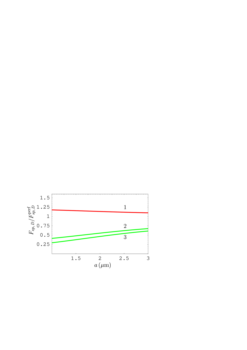
Figure 3: (Color online) The normalized Casimir force acting between an Au-coated spherical lens with surface imperfections of different types and an Au plate as a function of separation. Au is described by the Drude model. Lines 1, 2, and 3 are for the surface imperfections shown in Fig. 1(a,b,c), respectively.

Now we perform computations of the Casimir force between a real metal (Au) lens with a surface imperfection around the point of closest approach to a real metal (Au) plate normalized for the same force with a perfectly spherical lens. Note that in real experiments the lens and the plate are usually made of different materials coated with a metal layer. For lenses of centimeter-size curvature radius the thickness of an Au coating can be equal30 to about $0.5\,\mu$m. It was shown,51a however, that for Au layers of more than 30 nm thickness the Casimir force is the same as for test bodies made of bulk Au. First, we describe the metal of the lens and the plate by the Drude model with $\omega_{p}=9.0\,$eV and $\gamma=0.035\,$eV. Computations are performed by Eqs. (11) and (14) for imperfections in Fig. 1(a,b) and 1(c), respectively, with all parameters indicated in Sec. II, using Eqs. (23)–(25). The computational results for the quantity $F_{sp,D}(a,T)/F_{sp,D}^{\rm perf}(a,T)$ as a function of separation at $T=300\,$K are shown by lines 1, 2, and 3 in Fig. 3 for the surface imperfections presented in Fig. 1(a), (b), and (c), respectively. These lines are in qualitative agreement with respective lines in Fig. 2 for the ideal metal case. Thus, for the surface imperfection shown in Fig. 1(a) the assumption of a perfectly spherical surface of the lens leads to an underestimated Casimir force. As an example, for the imperfection in Fig. 1(a) the quantity $F_{sp,D}/F_{sp,D}^{\rm perf}$ at separations of 1 and $3\,\mu$m is equal to 1.176 and 1.097, respectively. Thus, the underestimation of the Casimir force varies from approximately 18% to 10%. The same quantity at the same respective separations is equal to 0.4125 and 0.6752 [for the surface imperfection in Fig. 1(b)] and 0.2951 and 0.6103 [for the surface imperfection in Fig. 1(c)]. This means that for the imperfection in Fig. 1(b) the assumption of perfect sphericity leads to an overestimation of the Casimir force which varies from 59% at $a=1\,\mu$m to 32% at $a=3\,\mu$m. For the surface imperfection in Fig. 1(c) the overestimation varies from 70% to 39% when separation increases from 1 to $3\,\mu$m. Thus, for real metals described by the Drude model surface imperfections of the lens surface play qualitatively the same role as for ideal metal lenses. As can be seen in Figs. 2 and 3, the lines labeled 1 for ideal metals and for Drude metals are markedly different, whereas the respective lines labeled 2 and 3 in both figures look rather similar. It is explained by the fact that for the surface imperfection shown in Fig. 1(a) $D_{1}=0.5\,\mu$m, while for the imperfections in Fig. 1(b,c) $D_{1}=1\,\mu$m. As a result, the influence of the model of the metal used (ideal metal or the Drude metal) for the lines labeled 2 and 3 is not so pronounced as for the line labeled 1. A few computational results for the quantity $F_{sp,D}^{\rm perf}$ at different separations for a lens with $R=15\,$cm are presented in column (a) of Table I. They are used below in this section. For comparison purposes in column (b) of Table I the same quantity is computed using the tabulated optical data for a complex index of refractionPalik1 extrapolated to low frequencies by means of the Drude model. As can be seen in Table I, the Casimir forces in columns (a) and (b) at each separation are almost coinciding. This confirms that at $a\geq 1\,\mu$m the role of interband transitions is negligibly small, as was noted in the beginning of this section.

Now we consider the lens and the plate made of metal described by the plasma model (26) and compute the quantity $F_{sp,p}(a,T)/F_{sp,p}^{\rm perf}(a,T)$ using Eqs. (11), (14) and (23), (24). It turns out that the computational results differ only slightly from respective results shown in Fig. 3. Because of this, Fig. 3 is in fact relevant to a lens and a plate made of a metal described by the plasma model as well. To illustrate minor differences arising when the plasma model is used, we present the following values of the quantity $F_{sp,p}/F_{sp,p}^{\rm perf}$ for all three types of surface imperfections shown in Fig. 1(a,b,c) at separations $a=1$ and $3\,\mu$m, respectively: 1.17 and 1.092 [imperfection of Fig. 1(a)]; 0.4333 and 0.6916 [imperfection of Fig. 1(b)]; 0.3200 and 0.6300 [imperfection of Fig. 1(c)]. Comparing these values with the above results obtained using the Drude model, we find that relative differences vary from a fraction of percent to a few percent. In column (c) of Table I we present several computational results for the quantity $F_{sp,p}^{\rm perf}$. Column (d) of the same table contains similar results computed using the generalized plasma-like model2 ; 3 ; 11 taking into account the interband transitions of core electrons. The results of columns (c) and (d) computed at the same separations are almost coinciding.

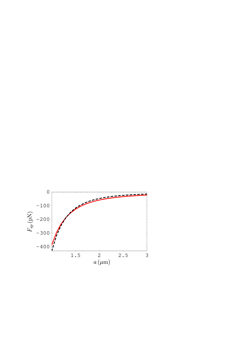
Figure 4: (Color online) The Casimir force between a perfectly spherical lens and a plate, both described by the plasma model, versus separation is shown by the solid line. The dashed line shows the same force between a sphere with some surface imperfection and a plate, both described by the Drude model. See text for further discussion.

Now we consider the situation when computational results for the Casimir force between a perfectly spherical lens above a plate, both described by the plasma model, are approximately the same as for a lens with some surface imperfection above a plate, both described by the Drude model (here and below we use the same Drude parameters for Au as already indicated in the text). In Fig. 4 the Casimir force $F_{sp,p}^{\rm perf}$ between a perfectly shaped lens of $R=15\,$cm radius of curvature and a plate versus separation is shown as the solid line [see also column (c) in Table I]. It is computed by Eqs. (6), (23), (24), and (26) at $T=300\,$K. As an alternative, we assume that there is a surface imperfection on the lens around the point of closest approach to the plate shown in Fig. 1(a). For the parameters of this imperfection (bubble) we choose $R_{1}=23\,$cm, $D_{1}=0.75\,\mu$m which leads to $r\approx 0.59\,$mm and $d\approx 1.16\,\mu$m. The flattening of the lens in this case is equal to $d-D_{1}\approx 0.41\,\mu$m, i.e., much smaller than the error in the measurement of lens curvature radius.

Computations of the Casimir force $F_{sp,D}$ between a lens with this imperfection and a plate as a function of separation are performed by Eqs. (11) and (23)–(25). The computational results are shown in Fig. 4 by the dashed line. At a few separations, these results are presented in Table I, column (e). As can be seen in Fig. 4, the values of the Casimir force for a perfectly spherical lens described by the plasma model are rather close to the force values for a lens with imperfection described by the Drude model. For example, using columns (c) and (e) in Table I, one obtains that the relative difference between the two descriptions

$$\delta F_{sp}(a,T)=\frac{F_{sp,p}^{\rm perf}(a,T)-F_{sp,D}(a,T)}{F_{sp,p}^{\rm perf}(a,T)}$$ (27)

varies from –11% at $a=1\,\mu$m to 34% at $a=3\,\mu$m. Keeping in mind that the error of force measurements quickly increases with the increase of separation, it appears impossible to make any definite conclusion on the model of dielectric properties from the extent of agreement between the experimental data and theory.

Now we consider the opposite situation, i.e., when the Casimir force $F_{sp,D}^{\rm perf}$ is approximately equal to $F_{sp,p}$ for a sphere with some imperfection over the separation region from 1 to $3\,\mu$m. The Casimir force $F_{sp,D}^{\rm perf}$ between a perfectly spherical lens of $R=15\,$cm radius of curvature and a plate, both described by the Drude model (25), was computed as a function of separation by Eqs. (6) and (23)–(25). The computational results are shown in Fig. 5(a) by the dashed line [see also column (a) in Table I]. Large deviation between the solid line in Fig. 4 and the dashed line in Fig. 5(a) reflects the qualitative difference between the theoretical descriptions of the Casimir force by means of the plasma and Drude models.

Approximately the same theoretical results, as shown by the dashed line in Fig. 5(a), can be obtained, however, for a lens and plate metal described by the plasma model if the lens surface possesses some specific imperfection near the point of closest approach to the plate. In Sec. II we have considered only the most simple surface imperfections. There may be more complicated imperfections on the lens surface, specifically, different combinations of imperfections shown in Fig. 1(a,b,c). In Fig. 5(b) we show the surface imperfection on the lens surface with $R=15\,$cm curvature radius consisting of two bubbles. The first bubble is of $R_{1}=3\,$cm radius of curvature. It is of the same type as that shown in Fig. 1(b). The second bubble on the bottom of the first is of $R_{2}=19\,$cm curvature radius. It is like that in Fig. 1(a). From Fig. 5(b) one obtains $D_{1}\approx 1.5\,\mu$m, $D_{2}\approx 0.2\,\mu$m, and $r\approx 0.47\,$mm. For the increase of lens thickness at the point of closest approach to the plate due to the presence of bubbles, we find $0.74\,\mu$m which is much smaller than the error in the measurement of the lens radius of curvature. The Casimir force between the spherical lens with two bubbles and a plate is given by the repeated application of Eq. (11) to each of the bubbles

$$F_{sp}(a,T)=2\pi(R_{1}-R_{2}){\cal F}_{pp}(a+D_{2},T)+2\pi R_{2}{\cal F}_{pp}(a,T)$$

$$~{}~{}~{}~{}~{}~{}~{}~{}~{}~{}~{}~{}+2\pi(R-R_{1}){\cal F}_{pp}(a+D_{1},T).$$ (28)

We performed numerical computations of the Casimir force $F_{sp,p}$ as a function of separation using Eqs. (23), (24), (26), and (28). The computational results are shown in Fig. 5(a) by the solid line. At a few separation distances these results are presented in TableI1, column (f). As can be seen in Fig. 5(a), the theoretical lines computed for a perfectly spherical lens using the Drude model and for a lens with a surface imperfection using the plasma model are rather close. Quantitatively from columns (a) and (f) in Table I one obtains that the quantity

$$\delta\tilde{F}_{sp}(a,T)=\frac{F_{sp,D}^{\rm perf}(a,T)-F_{sp,p}(a,T)}{F_{sp,D}^{\rm perf}(a,T)}$$ (29)

varies from –10% at $a=1\,\mu$m to 26% at $a=3\,\mu$m. Such small differences do not allow experimental resolution between alternative theoretical descriptions of the lens and plate material by means of the Drude and plasma models. The reason is that in experiments with lenses of centimeter-size radius of curvature at large separations, as explained in Sec. III, the experimental error exceeding a few tens of percent is expected.

V Metallic or semiconductor lens above a semiconductor plate

As mentioned in Sec. I, the account of relaxation properties of free charge carriers in semiconductor and dielectric materials also creates problems for the theoretical description of the thermal Casimir force. Here, most of experiments12 ; 21 ; 22 ; 25 ; 54 were performed with an Au-coated sphere of about $100\,\mu$m radius above a semiconductor plate, and only one 31 with a Ge spherical lens of $R=15.1\,$cm above a Ge plate. The measurement data of the two experiments 12 ; 13 are inconsistent with the inclusion of dc conductivity into a model of the dielectric response for high-resistivity semiconductors with the concentration of charge carriers below critical (i.e., for semiconductors of dielectric type whose conductivity goes to zero when temperature vanishes) and for dielectrics. The question of how to describe free charge carriers of low-resistivity semiconductors in the Lifshitz theory (e.g., by means of the Drude or plasma model) also remains unsolved. One may hope that these problems can be solved in experiments on measuring the Casimir force between large Au-coated or semiconductor lenses above semiconductor plates. Below we show, however, that invariably present imperfections of lens of large radius of curvature do not allow one to discriminate between the different theoretical models.

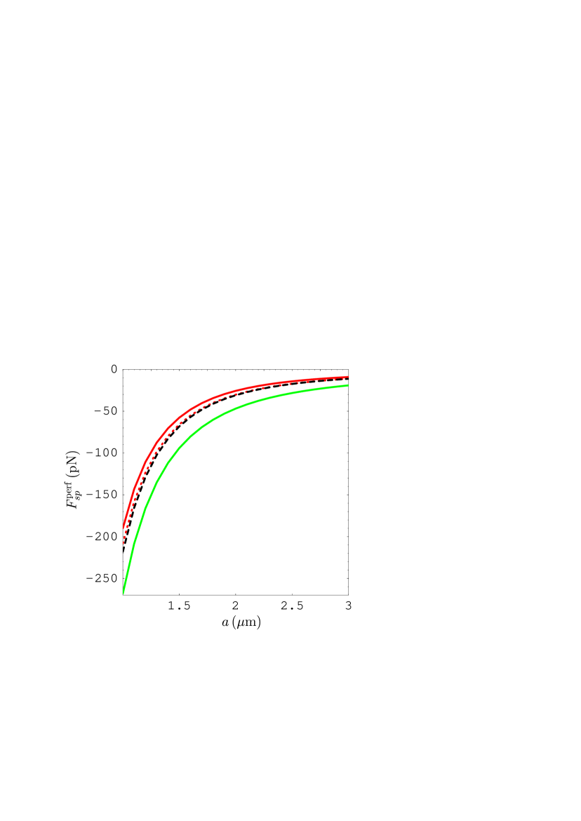
Figure 6: (Color online) The Casimir force between a perfectly spherical Au-coated lens and Si plate as a function of separation for dielectric Si (the upper solid line), dielectric Si with dc conductivity included (the dotted line), low-resistivity Si described by the Drude model (the dashed line), and low-resistivity Si described by the plasma model (the lower solid line).

We start with a perfectly spherical Au-coated lens of $R=15\,$cm curvature radius above a Si plate. Within the first model we describe a high-resistivity Si plate as a true dielectric with the dielectric permittivity $\varepsilon_{\rm Si}(\omega)$ determined from the tabulated optical data 55 for Si samples with the resistivity $\rho_{0}=1000\,\Omega\,$cm. In so doing $\varepsilon_{\rm Si}(0)=11.66<\infty$. This model is an approximation because it disregards the dc conductivity of Si. The computational results for the Casimir force between a lens and a plate computed using Eqs. (6), (23), and (24) with $\varepsilon_{l}=\varepsilon_{\rm Si}(i\omega_{c}\zeta_{l})$ at $T=300\,$K are shown by the upper solid line in Fig. 6. These results are almost independent of whether the Drude or the plasma model is used for the description of the lens metal. Specifically, the relative difference in force magnitudes due to the use of the Drude or plasma models decreases from 0.22% to 0.031% when the separation distance increases from 1 to $3\,\mu$m.

Within the second model we consider the same high-resistivity Si plate, but take the dc conductivity into account. Then the dielectric permittivity can be presented in the form

$$\varepsilon_{\rm Si}^{dc}(\omega)=\varepsilon_{\rm Si}(\omega)+i\frac{4\pi\sigma_{0}}{\omega},$$ (30)

where $\sigma_{0}=\sigma_{0}(T)$ is the static conductivity. In the local approximation the permittivity (30) correctly describes the reaction of semiconductors on real electromagnetic fields. In this case computations using Eqs. (6), (23), and (24) result in the dotted line in Fig. 6. Note that the computational results do not depend on the value of $\sigma_{0}$ in Eq. (30), but only from the fact that $\sigma_{0}\neq 0$. The dotted line in Fig. 6 is also almost independent on whether the Drude or the plasma model is used for the description of a lens metal.

As the third and fourth models we consider Si plate made of low-resistivity B doped Si with the concentration of charge carriers above the critical value. 21 This is a semiconductor of metallic type whose conductivity does not go to zero when the temperature vanishes. We present the dielectric permittivity of such a plate in the form (the third model)

$$\varepsilon_{\rm Si}^{D}(\omega)=\varepsilon_{\rm Si}(\omega)-\frac{\omega_{p,\,\rm Si}^{2}}{\omega(\omega+i\gamma_{\rm Si})},$$ (31)

where the values of the Drude parameters are 21 $\omega_{p,\,\rm Si}\approx 0.46\,$eV and $\gamma_{\rm Si}\approx 0.099\,$eV, or in the form (the fourth model)

$$\varepsilon_{\rm Si}^{p}(\omega)=\varepsilon_{\rm Si}(\omega)-\frac{\omega_{p,\,\rm Si}^{2}}{\omega^{2}}.$$ (32)

The results of the computations using Eqs. (6), (23), (24), and either (31) or (32) are presented in Fig. 6 by the dashed and lower solid lines, respectively. Similar to models used for the description of low-resistivity Si, the metallic lens was described by the Drude model [when Si was described by Eq. (31)] or by the plasma model [for the dielectric permittivity of Si in Eq. (32)]. Note that the magnitudes of the Casimir forces given by the second and third models (the dotted and dashed lines in Fig. 6, respectively) are very close. When separation increases from 1 to $3\,\mu$m, the relative differences between the dotted and dashed lines decrease from 4.8% to 0.75%, respectively. Figure 6 demonstrates that the magnitudes of the Casimir force between an Au lens and a Si plate may vary over a wide range depending on the choice of a Si sample and theoretical model used.

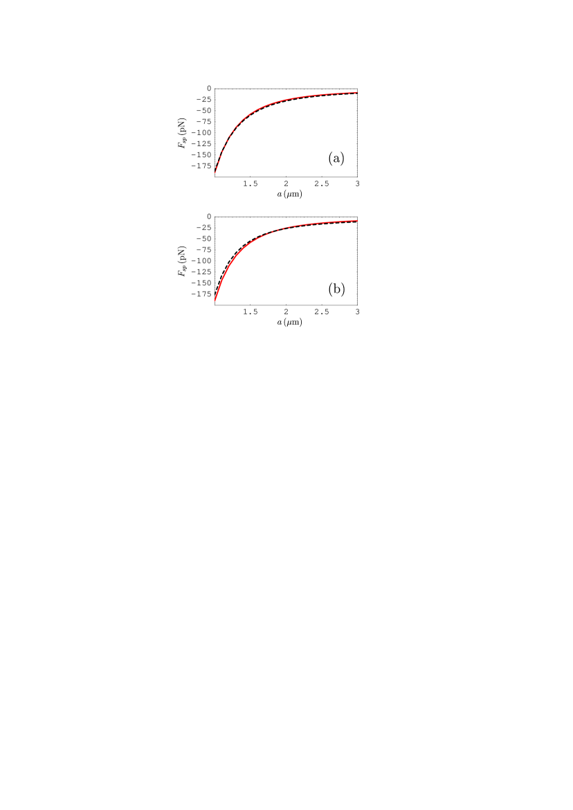
Figure 7: (Color online) The Casimir force between a perfectly spherical Au-coated lens and Si plate made of dielectric Si versus separation is shown by the solid lines. The dashed lines show the Casimir force between an Au-coated lens with some specific surface imperfections and a plate made of low-resistivity Si where Si is described (a) by the Drude model and (b) by the plasma model.

Now we present a few computational results for the Casimir force between an Au-coated lens and a Si plate when the Si is described by the different models listed above and the lens may have surface imperfections around the point of closest approach to the plate. We first consider the plate made of dielectric Si (the first model) described by the dielectric permittivity $\varepsilon_{\rm Si}(\omega)$ and the Au-coated lens of perfect sphericity. The Casimir force in this case is shown by the solid line in Fig. 7(a) which was already presented in Fig. 6 as the upper solid line. Now let the plate be made of low-resistivity Si described by the Drude dielectric permittivity (31) (the third model) and the lens possess the surface imperfection shown in Fig. 1(b) with the parameters $R_{1}=12.5\,$cm, $D_{1}=1\,\mu$m, $r\approx 0.5\,$mm. The results of the numerical computations for the Casimir force using Eqs. (11), (23)–(25), and (31) are shown by the dashed line in Fig. 7(a). As is seen from this figure, the dashed line is almost coinciding with the solid one. Thus, the relative deviation of the Casimir force for a lens with surface imperfection from the force with a perfectly spherical lens [defined similar to Eqs. (27) and (29)] varies from –2% to 13% when separation increases from 1 to $3\,\mu$m. Because of this, with lenses of large radius of curvature it is not possible to experimentally resolve between the case of high-resistivity (dielectric) Si described by the finite dielectric permittivity $\varepsilon_{\rm Si}(\omega)$ and low-resistivity Si described by the Drude model. Almost the same Casimir forces, as shown by the dashed line in Fig. 7(a), are obtained for a plate made of high-resistivity Si with dc conductivity included in accordance with Eq. (30) (the second model) if the lens has an imperfection shown in Fig. 1(b) with the parameters $R_{1}=13\,$cm, $D_{1}=1\,\mu$m, $r\approx 0.5\,$mm. In this case the Casimir force for a lens with surface imperfection deviates from the force for a perfectly spherical lens by –3% at $a=1\,\mu$m and 14% at $a=3\,\mu$m.

The last, fourth, model to discuss is of the plate made of low-resistivity Si described by the plasma dielectric permittivity (32). In this case we consider an Au-coated sphere with surface imperfection (two bubbles) shown in Fig. 5(b). The parameters of the imperfection are the following: $R_{1}=1.5\,$cm, $R_{2}=21\,$cm, $D_{1}=2\,\mu$m, $D_{2}=0.2\,\mu$m leading to $r\approx 0.28\,$mm. Computations of the Casimir force are performed using Eqs. (23), (24), (26), and (32). The computational results are shown as the dashed line in Fig. 7(b). In the same figure the solid line reproduces the Casimir force acting between a perfectly spherical lens and a plate made of dielectric Si. The relative differences between the dashed and solid lines in Fig. 7(b) vary from –8% to 23% when the separation increases from 1 to $3\,\mu$m. Thus, experimentally it would be not possible to distinguish between the cases when the lens surface is perfectly spherical and the plate is made of dielectric Si, and when the lens surface has an imperfection, but Si plate is of low-resistivity and is described by the plasma model.

In the end of this section we briefly consider the spherical lens of $R=15.1\,$cm radius made of intrinsic Ge above the plate made of the same semiconductor.31 In this experiment, Eq. (6) was used31 for the comparison between the measurement data and theory. As two simple examples we consider that the Ge lens has a bubble either of the radius of curvature $R_{1}=22\,$cm and thickness $D_{1}=0.09\,\mu$m or $R_{1}=10\,$cm and thickness $D_{1}=0.2\,\mu$m near the point of closest approach to a Ge plate [see Fig. 1(a) and (b), respectively]. The radii of the two bubbles are coinciding and equal to $r=0.2\,$mm leading to the diameter of each of the bubbles $2r=0.4\,$mm (see Sec. II). The obtained value should be compared with limitations imposed by the scratch/dig optical surface specification data of the used31 Ge lens of ISP optics, GE-PX-25-50. According to the information from the producer,530a this lens has the surface quality 60/40. The latter means that 0.4 mm is just the maximum diameter of bubbles allowed. It is also easily seen that the flattening of the lens surface in Fig. 1(a) or the swelling up in Fig. 1(b) due to bubbles are much less than the absolute error of $R$ equal to31 $\Delta R=0.05\,$cm. Really, with the above parameters $d\approx 0.13\,\mu$m. As a result, the flattening of the lens surface in Fig. 1(a) is given by $d-D_{1}\approx 0.04\,\mu$m and the swelling up in Fig. 1(b) is given by $D_{1}-d\approx 0.07\,\mu$m. In the presence of bubbles the Casimir force should be calculated not by Eq. (6) but by Eq. (11). Computations using the dielectric permittivity530b of intrinsic Ge show that for the used parameters of the bubble in Fig. 1(a) Eq. (11) leads to larger magnitudes of the Casimir force by 15% and 10% than Eq. (6) at separations $a=0.6$ and $1\,\mu$m, respectively. On the opposite, for the bubble in Fig. 1(b) the use of Eq. (11) instead of Eq. (6) results in smaller magnitudes of the Casimir force by 19% and 14% at the same respective separations.

VI Conclusions and discussion

In the foregoing we have investigated the impact of imperfections, which are invariably present on lens surfaces of centimeter-size radius of curvature, on the Casimir force in the lens-plate geometry. We have demonstrated that if an imperfection in the form of a bubble or a pit is located near the point of the closest approach of a lens and a plate, the impact on the Casimir force can be dramatic. We first considered a metal-coated lens above a metal-coated plate. It was shown that the Casimir force between a perfectly spherical lens and a plate, both described by the plasma model, can be made approximately equal to the force between a sphere with some surface imperfection and a plate, both described by the Drude model. Similarly, the Casimir force computed for a perfectly spherical lens and a plate described by the Drude model can be approximately equal to the force computed for a lens with surface imperfection and a plate described by the plasma model. In both cases the approximate equality of forces in the limits of the error of force measurements was found over a wide range of separations from 1 to $3\,\mu$m. The absolute impact of surface imperfections on the lens surfaces of centimeter-size radii of curvature on the Casimir force is on the order of a few tens of percent for both ideal and real metals. Surface imperfections can lead to both a decrease and an increase of the force magnitude. These conclusions obtained by simultaneous consideration of the Drude and plasma models are of major importance for experiments aiming to discriminate between the predictions of both approaches at separations above $1\,\mu$m and to resolve the long-term controversy in the theoretical description of thermal Casimir forces.

The above conclusions were obtained using the spatially local Drude and plasma dielectric functions. The possible impact of nonlocal dielectric permittivity on the thermal Casimir force between metallic test bodies was investigated in detail in the literature. Specifically, it was shown53a that even for metal coatings thinner than the mean free path of electrons in the bulk metal, the relative difference in the thermal Casimir forces computed using the local Drude model and nonlocal permittivities is less than a few tenth of a percent ($\approx 0.2$% at $a=100\,$nm and decreases with the increase of separation). For thicker metal coatings used in experiments the contribution of nonlocal effects to the thermal Casimir force further decreases. This is explained by the fact that the use of nonlocal dielectric permittivities leads53b ; 53c to the same equality, $r_{\rm TE}(0,k_{\bot})=0$, as does the Drude model (18). Thus, there is no need to consider nonlocal dielectric functions in connection with surface imperfections of lenses with centimeter-size curvature radii. For other fluctuation phenomenon, as radiative heat transfer, it was also calculated41b that at separations between two metallic semispaces $a>100\,$nm the contribution of nonlocal effects into the heat flux is very small.

Similar results were obtained for an Au-coated lens of centimeter-size radius of curvature above a Si plate. It was shown that different models for the description of charge carriers in Si (dielectric Si, high-resistivity Si with account of dc conductivity, low-resistivity Si described by the Drude model, and low-resistivity Si described by the plasma model) lead to different theoretical predictions for the Casimir force between a perfectly spherical Au-coated lens and a Si plate. However, by choosing an appropriate imperfection, well within the optical surface specification data, on the surface of the lens at the point of closest approach to the plate it is possible to obtain approximately the same Casimir forces in all the above models over the separation region from 1 to $3\,\mu$m.

The above results show that the presently accepted approach to the comparison of the data and theory in experiments30 ; 31 ; 29a ; 29aa measuring the Casimir force by means of lenses with centimeter-size radii of curvature might be not sufficiently justified. In these experiments the Casimir force is computed using the simplest formulation of the PFA in Eq. (6), i.e., under an assumption of perfect sphericity of the lens surface. According to our results, however, Eq. (6) is not applicable in the presence of surface imperfections which are invariably present on lens surfaces. In fact, for reliable comparison between the measurement data and theory it would be necessary, first, to determine the position of the point of closest approach to the plate on the lens surface with a precision of a fraction of micrometer. Then one could investigate the character of local imperfections in the vicinity of this point microscopically and derive an approximate formulation of the PFA like in Eqs. (11), (14) or (28). Thereafter the measurement data could be compared with theory with some degree of certainty. It is unlikely, however, that sufficiently precise determination of the point of closest approach to the plate is possible for lenses of centimeter-size radii of curvature. The possibility to return to the same point of closest approach in repeated measurements is all the more problematic. Because of this, one can conclude that measurements of the Casimir force using lenses of centimeter-size radii of curvature do not allow an unambiguous comparison to theory, and are not reproducible (see Refs.30 ; 29a ; 29aa whose results are mutually contradictory). According to our results, even if the measurement data for the Casimir force are not consistent with any theoretical model under an assumption of perfect sphericity of the lens surface, there might be different types of surface imperfections leading to the consistency of the data with several theoretical approaches.

We emphasize that only a few simple surface imperfections in the form of bubbles and pits are considered in this paper. There are many other imperfections of a more complicated shape (including scratches) which are allowed by the optical surface specification data and may strongly impact on the Casimir force between a centimeter-size lens and a plate. Such imperfections are randomly distributed on lens surfaces and some of them can be located in the immediate region of the point of closest approach to the plate. The role of Au coatings used in measurements of the Casimir force, should be investigated as well in the presence of surface imperfections. Metallic coating of about $0.5\,\mu$m thickness 30 might lead to a decrease of thicknesses of bubbles and depths of pits, but to an increase of their diameters. The latter, however, influences the magnitude of the Casimir force most dramatically.

The above discussed fundamental problem arising in the measurements of the Casimir force using lenses of centimeter-size curvature radii does not arise for microscopic spheres of about $100\,\mu$m radii used in numerous experiments by different authors performed with the help of an atomic force microscope 2 ; 17 ; 19 ; 3 ; 12 ; 18 ; 20 ; 21 ; 22 ; 23 ; 27 ; 28 ; 29 ; 34 ; 54 and micromechanical torsional oscillator.2 ; 9 ; 26 ; 3 ; 10 ; 11 ; 24 ; 25 For instance, for microscopic polystyrene spheres made by the solidification from the liquid phase the minimization of surface energy leads to perfectly smooth spherical surfaces due to surface tension. The surface quality of such spheres after metallic coating was investigated using a scanning electron microscope 2 ; 17 ; 3 and did not reveal any bubbles or scratches. Spheres of microscopic size have been successfully used 9 ; 10 ; 11 to exclude large thermal effect in the Casimir force at separations below $1\,\mu$m. They are, however, not suitable for measurements of the thermal effect at large separations of a few micrometers because the Casimir force is proportional to the sphere radius and rapidly decreases with the increase of separation. Keeping in mind the above discussed fundamental problem arising for spherical lenses of centimeter-size radius of curvature, the only remaining candidate for the measurement of thermal effect in the Casimir force at micrometer separations is the classical Casimir configuration of two parallel plates.58

Figure 1: (Color online) The configuration of a spherical lens with radius of curvature $R$ possessing a surface imperfection around the point of closest approach to a plate. (a) The bubble radius of curvature is $R_{1}>R$. (b) The bubble radius of curvature is $R_{1}<R$. (c) The pit radius of curvature is $R_{1}<R$. The relative sizes of the lens and imperfection are not shown to scale.

                      

                      

                      

                 

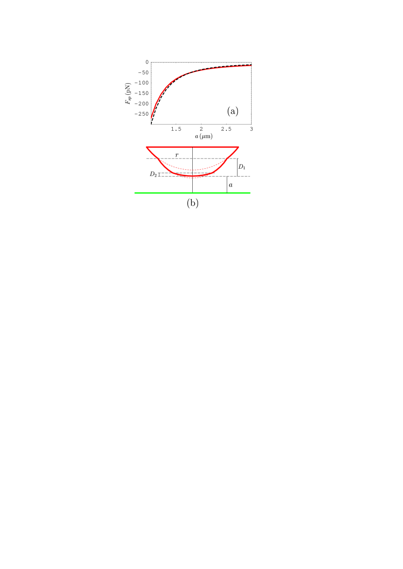
Figure 5: (Color online) (a) The Casimir force between a perfectly spherical lens and a plate, both described by the Drude model, versus separation is shown by the dashed line. The solid line shows the same force between a sphere with some surface imperfection and a plate, both described by the plasma model. See text for further discussion. (b) The configuration of a spherical lens with radius of curvature $R$ possessing a surface imperfection in the form of two bubbles around the point of closest approach to a plate. The relative sizes of the lens and imperfection are shown not to scale.

                      

             

Table 1: The values of the Casimir force between an Au-coated sphere of $R=15\,$cm radius of curvature and an Au-coated plate computed at $T=300\,$K for (a) Au described by the Drude model and a perfectly shaped lens; (b) Au described by the tabulated optical data extrapolated by means of the Drude model and a perfectly shaped lens; (c) Au described by the plasma model and a perfectly shaped lens; (c) Au described by the generalized plasma-like model and a perfectly shaped lens; (e) Au described by the Drude model and a lens with surface imperfection shown in Fig. 1(a); (e) Au described by the plasma model and a lens with surface imperfection shown in Fig. 5(b). See text for the parameters of lens imperfections.

$a$	$F_{sp}(a)$ (pN)
($\mu$m)	(a)	(b)	(c)	(d)	(e)	(f)
1.0	–299.08	–299.38	–386.56	–386.64	–430.34	–269.93
1.5	–84.914	–84.953	–124.44	–124.44	–116.72	–80.423
2.0	–35.540	–35.548	–57.984	–57.985	–46.681	–37.298
2.5	–18.874	–18.876	–33.330	–33.331	–27.787	–21.961
3.0	–11.744	–11.745	–21.830	–21.830	–14.304	–14.847

References

- (1) H. B. G. Casimir, Proc. K. Ned. Akad. Wet. 51, 793 (1948).
- (2) M. Bordag, G. L. Klimchitskaya, U. Mohideen, and V. M. Mostepanenko, Advances in the Casimir Effect (Oxford University Press, Oxford, 2009).
- (3) U. Mohideen and A. Roy, Phys. Rev. Lett. 81, 4549 (1998).
- (4) B. W. Harris, F. Chen, and U. Mohideen, Phys. Rev. A 62, 052109 (2000).
- (5) R. S. Decca, E. Fischbach, G. L. Klimchitskaya, D. E. Krause, D. López, and V. M. Mostepanenko, Phys. Rev. D 68, 116003 (2003).
- (6) M. Lisanti, D. Iannuzzi, and F. Capasso, Proc. Natl. Acad. Sci. USA 102, 11989 (2005).
- (7) G. L. Klimchitskaya, U. Mohideen, and V. M. Mostepanenko, Rev. Mod. Phys. 81, 1827 (2009).
- (8) E. M. Lifshitz, Zh. Eksp. Teor. Fiz. 29, 94 (1956) [Sov. Phys. JETP 2, 73 (1956)].
- (9) E. M. Lifshitz and L. P. Pitaevskii, Statistical Physics, Part. II (Pergamon Press, Oxford, 1980).
- (10) M. Boström and B. E. Sernelius, Physica A 339, 53 (2004).
- (11) B. Geyer, G. L. Klimchitskaya, and V. M. Mostepanenko, Phys. Rev. D 72, 085009 (2005).
- (12) B. Geyer, G. L. Klimchitskaya, and V. M. Mostepanenko, Ann. Phys. (N.Y.) 323, 291 (2008).
- (13) R. S. Decca, D. López, E. Fischbach, G. L. Klimchitskaya, D. E. Krause, and V. M. Mostepanenko, Ann. Phys. (N.Y.) 318, 37 (2005).
- (14) R. S. Decca, D. López, E. Fischbach, G. L. Klimchitskaya, D. E. Krause, and V. M. Mostepanenko, Phys. Rev. D 75, 077101 (2007); Eur. Phys. J. C 51, 963 (2007).
- (15) F. Chen, G. L. Klimchitskaya, V. M. Mostepanenko, and U. Mohideen, Optics Express 15, 4823 (2007); Phys. Rev. B 76, 035338 (2007).
- (16) J. M. Obrecht, R. J. Wild, M. Antezza, L. P. Pitaevskii, S. Stringari, and E. A. Cornell, Phys. Rev. Lett. 98, 063201 (2007).
- (17) G. L. Klimchitskaya and V. M. Mostepanenko, J. Phys. A: Math. Theor. 41, 312002(F) (2008).
- (18) A. Roy, C.-Y. Lin, and U. Mohideen, Phys. Rev. D 60, 111101(R) (1999).
- (19) F. Chen, U. Mohideen, G. L. Klimchitskaya, and V. M. Mostepanenko, Phys. Rev. Lett. 88, 101801 (2002); Phys. Rev. A 66, 032113 (2002).
- (20) F. Chen, U. Mohideen, G. L. Klimchitskaya, and V. M. Mostepanenko, Phys. Rev. A 72, 020101(R) (2005); ibid 74, 022103 (2006).
- (21) F. Chen, G. L. Klimchitskaya, V. M. Mostepanenko, and U. Mohideen, Phys. Rev. Lett. 97, 170402 (2006).
- (22) H.-C. Chiu, G. L. Klimchitskaya, V. N. Marachevsky, V. M. Mostepanenko, and U. Mohideen, Phys. Rev. B 80, 121402(R) (2009); ibid 81, 115417 (2010).
- (23) H. B. Chan, V. A. Aksyuk, R. N. Kleiman, D. J. Bishop, and F. Capasso, Science 291, 1941 (2001); Phys. Rev. Lett. 87, 211801 (2001).
- (24) H. B. Chan, Y. Bao, J. Zou, R. A. Cirelli, F. Klemens, W. M. Mansfield, and C. S. Pai, Phys. Rev. Lett. 101, 030401 (2008).
- (25) G. Jourdan. A. Lambrecht, F. Comin, and J. Chevrier, Europhys. Lett. 85, 31001 (2009).
- (26) P. J. van Zwol, G. Palasantzas, M. van de Schootbrugge, and J. T. M. De Hosson, Appl. Phys. Lett. 92, 054101 (2008).
- (27) P. J. van Zwol, G. Palasantzas, and J. T. M. De Hosson, Phys. Rev. B 77, 075412 (2008).
- (28) S. K. Lamoreaux, Phys. Rev. Lett. 78, 5 (1997); ibid 81, 5475(E) (1998).
- (29) W. J. Kim, A. O. Sushkov, D. A. R. Dalvit, and S. K. Lamoreaux, Phys. Rev. Lett. 103, 060401 (2009).
- (30) A. O. Sushkov, W. J. Kim, D. A. R. Dalvit, and S. K. Lamoreaux, e-Print arXiv:1011.5219v1.
- (31) M. Masuda and M. Sasaki, Phys. Rev. Lett. 102, 171101 (2009).
- (32) http://www.prhoffman.com/technical/scratch-dig.htm
- (33) http://www.cidraprecisionservices.com/technical-information/scratch-dig.html
- (34) http://www.ispoptics.com/PDFs/PDFCatalog/Page55.pdf
- (35) J. H. McLeod and W. T. Sherwood, J. Opt. Soc. Am. 35, 136 (1945).
- (36) D. Liu, Y. Yang, L. Wang, Y. Zhuo, C. Lu, L. Yang, and R. Li, Opt. Comm. 278, 240 (2007).
- (37) J. M. Bernett, Meas. Sci. Technol. 3, 1119 (1992).
- (38) Z. Zhong, J. Mater. Process. Technol. 122, 173 (2002).
- (39) M. Young, Appl. Opt. 25, 1922 (1986).
- (40) R. E. Fisher, B. Tadic-Galeb, and P. R. Yoder, Optical System Design, 2nd Edn. (McGrow-Hill, Columbus, 2008).
- (41) W. J. Kim, M. Brown-Hayes, D. A. R. Dalvit, J. H. Brownell, and R. Onofrio, Phys. Rev. A 78, 020101(R) (2008).
- (42) W. J. Kim, M. Brown-Hayes, D. A. R. Dalvit, J. H. Brownell, and R. Onofrio, J. Phys. Conf. Ser. 161, 012004 (2009).
- (43) S. de Man, K. Heeck, and D. Iannuzzi, Phys. Rev. A 79, 024102 (2009).
- (44) R. S. Decca, E. Fischbach, G. L. Klimchitskaya, D. E. Krause, D. López, U. Mohideen, and V. M. Mostepanenko, Phys. Rev. A 79, 026101 (2009).
- (45) Q. Wei, D. A. R. Dalvit, F. C. Lombardo, F. D. Mazzitelli, and R. Onofrio, Phys. Rev. A 81, 052115 (2010).
- (46) J. Błocki, J. Randrup, W. J. Swiatecki, and C. F. Tsang, Ann. Phys. (N.Y.) 105, 427 (1977).
- (47) B. V. Derjaguin, Kolloid. Z. 69, 155 (1934).
- (48) B. Geyer, G. L. Klimchitskaya, and V. M. Mostepanenko, Phys. Rev. A 82, 032513 (2010).
- (49) A. Canaguier-Durand, P. A. Maia-Neto, A. Lambrecht, and S. Reynaud, Phys. Rev. Lett. 104, 040403 (2010).
- (50) A. Canaguier-Durand, P. A. Maia-Neto, A. Lambrecht, and S. Reynaud, Phys. Rev. A 82, 012511 (2010).
- (51) R. Zandi, T. Emig, and U. Mohideen, Phys. Rev. B 81, 195423 (2010).
- (52) K. A. Milton, The Casimir Effect (World Scientific, Singapore, 2001).
- (53) M. Bordag, B. Geyer, G. L. Klimchitskaya, and V. M. Mostepanenko, Phys. Rev. D 58, 075003 (1998).
- (54) L. D. Landau, E. M. Lifshitz, and L. P. Pitaevskii, Electrodynamics of Continuous Media (Pergamon Press, Oxford, 1984).
- (55) J. D. Jackson, Classical Electrodynamics, 3rd Edn. (Wiley, New York, 1999).
- (56) A. I. Volokitin and B. N. J. Persson, Rev. Mod. Phys. 79, 1291 (2007).
- (57) V. B. Bezerra, R. S. Decca, E. Fischbach, G. L. Klimchitskaya, D. E. Krause, D. López, V. M. Mostepanenko, and C. Romero, Phys. Rev. E 73, 028101 (2006).
- (58) V. M. Mostepanenko, V. B. Bezerra, R. S. Decca, B. Geyer, E. Fischbach, G. L. Klimchitskaya, D. E. Krause, D. López, and C. Romero, J. Phys. A 39, 6589 (2006).
- (59) V. B. Bezerra, G. Bimonte, G. L. Klimchitskaya, V. M. Mostepanenko, and C. Romero, Eur. Phys. J. C 52, 701 (2007).
- (60) I. Brevik, J. B. Aarseth, J. S. Høye, and K. A. Milton, Phys. Rev. E 71, 056101 (2005).
- (61) J. S. Høye, I. Brevik, J. B. Aarseth, and K. A. Milton, J. Phys. A: Math. Gen. 39, 6031 (2006).
- (62) J. S. Høye, I. Brevik, S. A. Ellingsen, and J. B. Aarseth, Phys. Rev. E 75, 051127 (2007).
- (63) G. Bimonte, Phys. Rev. A 79, 042107 (2009).
- (64) F. Intravaia and C. Henkel, Phys. Rev. Lett. 103, 130405 (2009).
- (65) B. E. Sernelius, Phys. Rev. A 80, 043828 (2009).
- (66) V. M. Mostepanenko and G. L. Klimchitskaya, Int. J. Mod. Phys. A 25, 2302 (2010).
- (67) G. L. Klimchitskaya, U. Mohideen, and V. M. Mostepanenko, Phys. Rev. A 61, 062107 (2000).
- (68) Handbook of Optical Constants of Solids, Vol. 1, ed. E. D. Palik (Academic, New York, 1985).
- (69) S. deMan, K. Heeck, R. J. Wijngaarden, and D. Iannuzzi, Phys. Rev. Lett. 103, 040402 (2009).
- (70) Handbook of Optical Constants of Solids, Vol. 2, ed. E. D. Palik (Academic, New York, 1991).
- (71) G. L. Klimchitskaya, e-print arXiv:0902.4254v2.
- (72) R. Esquivel-Sirvent and V. B. Svetovoy, Phys. Rev. B 72, 045443 (2005).
- (73) V. B. Svetovoy and R. Esquivel, Phys. Rev. E 72, 036113 (2005).
- (74) V. B. Svetovoy, Phys. Rev. Lett. 101, 163603 (2008).
- (75) P. Antonini, G. Bimonte, G. Bressi, G. Carugno, G. Galeazzi, G. Messineo, and G. Ruoso, J. Phys.: Conf. Ser. 161, 012006 (2009).