Magnetic measurement of the critical current anisotropy in coated conductors

Abstract

We determine the critical current anisotropy at maximum Lorentz force from hysteresis loops in a vibrating sample magnetometer. To eliminate the signal of spurious variable Lorentz force currents it is sufficient to cut the sample to a specific length, which is calculated from the position dependent sensitivity of the instrument. The procedure increases the resolution of the measurement and the results compare well to transport data on the same sample. As the electric field in magnetisation measurements is lower than in transport experiments the anisotropy at high currents (low temperatures and fields) can be measured without the need of making current contacts or any special sample preparation.

I Introduction

Current transport is the principal application of superconducting films and it is therefore straightforward to carry out transport measurements of the critical current density ($J_{\mathrm{c}}$), but certain limitations make an alternative characterisation method desirable. First, the resistive heat produced by the current contacts inhibits the measurement of the very high critical currents occuring at low temperatures and fields. Second, the electric field is rather high due to the limited voltage resolution on short test samples and the conductor is therefore even more prone to thermal instabilities. Magnetisation measurements solve the above problems: the experiment is contact-less and the electric field, which is defined by the sweep rate of the applied magnetic field, is about one order of magnitude lower than in transport measurements (see below).

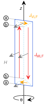
Figure 1: Geometry of the measurement. The magnetic field $H$ is perpendicular to the $z$-axis, which is the direction of the sample motion in the VSM and the axis of rotation ($\theta=0^{\circ}$ if $H$ is perpendicular to the film). The extended Bean model accounts for two different $a$,$b$-plane current densities flowing under maximum Lorentz force ($J_{\mathrm{MLF}}$) along the tape or under variable Lorentz force ($J_{\mathrm{VLF}}$) when closing the loop at the end. The labels mark the $z$-range, where the VLF-currents flow (see Fig. 2).

Due to the geometry of magnetisation measurements (see Fig. 1) it is, however, impossible to obtain the $J_{\mathrm{c}}$ anisotropy under the same well defined conditions as in transport experiments. If a conductor is rotated around its long axis in a magnetic field applied perpendicular to the axis of rotation, the induced currents flow in the $a,b$-plane, which is a consequence of the thin film geometry, but they flow under different forces: the currents directed along the tape flow always at right angles to the magnetic field—a configuration identical to transport measurements at maximum Lorentz force (MLF); the currents closing the loop at the end of the tape flow under variable Lorentz force (VLF). As a consequence, the tape carries two different critical current densities, which cannot be extracted from the measurement of a single quantity, i.e., the magnetic moment of the tape.

These spurious VLF-currents must therefore be eliminated to substitute transport by magnetisation measurements. One possibility is to pattern the conductor into many strips, which increases the length-to-width aspect ratio and decreases the contribution of the VLF-currents to the magnetic moment.Thompson et al. (2010) Apart from the additional experimental effort the striation reduces the total magnetic moment of the sample $m\propto w^{2}/n$ ($w$ is the original width, $n$ the number of cuts) at the expense of the resolution of the measurement.

In the following we will show that it is sufficient to cut the conductor to a certain length when measuring in a transverse vibrating sample magnetometer (VSM). The method is simple and increases the resolution of the measurement.

II Method

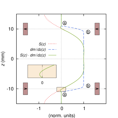
Figure 2: A Mallinson coil-set consists of two pairs of coils (brown rectangles) with opposite winding direction (indicated by the arrows). The VSM sensitivity $S(z)$ is positive between the coils and changes sign approximately at the $z$-position of the pick-up coils. The VLF-currents start to flow where $dm/dz(z)$ decreases to zero. (Confer Fig. 1 for the label positions.) If this area of the sample is at a position, where $S(z)$ is small and changes sign, the contribution of the VLF-currents to the total signal, which is proportional to the area under $S(z)\cdot{}dm/dz(z)$, is drastically reduced. The inset is a magnification of the area, where the VLF-currents close the loop.

Our approach is based on the fact that the sensitivity of a VSM equipped with a Mallinson coil set Mallison (1966) (the standard pick-up coil geometry) depends on the position of the magnetic moment. For our approach it is sufficient to take only the $z$-dependence into account. The convolution of the line density of magnetic moments $dm/dz(z)=\int\!\!\int dxdy\,M(x,y,z)$ along the $z$-dimension of the sample with the VSM sensitivity function $S(z)$ is the VSM output signal

$$V(z)=\int dz^{\prime}\,S(z^{\prime})\,dm/dz(z-z^{\prime})\;.$$ (1)

(Here, $z$ refers to the distance between the centre of the sample and the centre of the coil set.) If a small sample ($dm/dz(z)=m\,\delta(z)$ for a magnetic dipole) is scanned along the $z$-axis, $V(z)\propto S(z)$: the symmetric function is positive approximately up to the position of the pick-up coils and becomes negative outside (see Fig. 2). Measuring a small sample at the centre position determines the calibration constant $\alpha=1/S(0)$ in $m=\alpha\,V(0)$.

If the $z$-extension of the sample can’t be neglected, the convolution Equation 1 comes into effect, the above calibration is invalid and we have to distinguish between the real magnetic moment $m_{\mathrm{r}}=\int dz\,dm/dz(z)$ of the sample and the magnetic moment sensed by the instrument $m_{\mathrm{s}}=\alpha V(0)$. On the other hand, we can take advantage of the $z$-dependence of the VSM sensitivity: if the spurious VLF-currents at the end of the film are close to the pick-up coils, where $S(z)$ is small and changes sign, their net contribution to $m_{\mathrm{s}}$ can be eliminated (see Fig. 2). At the same time the signal of the MLF-currents and the resolution of the measurement increase, because the currents span the region with positive $S(z)$ between the coils.

The optimal sample length (defined below) and the new calibration constant $\alpha^{\star}$, are available from Eqn. 1. The sensitivity function $S(z)$ can be calculated Lacey et al. (1995) or measured (see above); integrating the magnetisation $M(x,y,z)$ of a film with two constant critical current densities ($J_{\mathrm{MLF}}$ and $J_{\mathrm{VLF}}$ in the extended Bean model sketched in Fig. 1) across the width and the thickness results in $dm/dz(z)$.

We define the optimum sample length as the length, where the sensitivity of the VSM to VLF-currents becomes minimal. For quantification we consider two limiting cases: the sensed magnetic moment when the field is applied perpendicular and parallel to the film plane. In the first case both current densities are equal, but for all other directions of the magnetic field $J_{\mathrm{VLF}}$ will exceed $J_{\mathrm{MLF}}$. We assume the worst case and let the ratio $R=J_{\mathrm{VLF}}/J_{\mathrm{MLF}}$ diverge, if the field is in-plane and the VLF-currents are force free. Evaluating the upper limit of the relative measurement error

$$\epsilon(l)=|m_{\mathrm{s}}(l,R=1)-m_{\mathrm{s}}(l,R\rightarrow\infty)|/m_{\mathrm{s}}(l,R=1)$$ (2)

as a function of the sample length $l$ quantifies the sensitivity of the VSM to changes in $J_{\mathrm{VLF}}$.

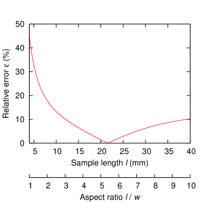
Figure 3: Calculated relative measurement error as a function of the sample length. Cutting the sample to the optimum length reduces the error to below 1 % and makes the VSM insensitive to changes of the VLF-currents.

For a 4 mm wide coated conductor we find an optimum length of 22 mm after calculating $S(z)$ from theory and fitting the positions of the pick-up-coils to a measurement of $V(z)\propto S(z)$ in our Oxford Instruments MagLab VSM using a small calibration sample. The maximum relative error is below 1 % at the optimum length (see Fig. 3) and the influence of the VLF-currents can be disregarded in the evaluation of $J_{\mathrm{MLF}}$, because the VSM is now insensitive to changes of $J_{\mathrm{VLF}}$.

We determine the anisotropy $J_{\mathrm{c}}(\theta)$ at maximum Lorentz force from the width of the hysteresis using the signals of two coil-sets parallel and orthogonal to the direction of the applied magnetic field

$$m_{\mathrm{s}}=\sqrt{\Delta m_{\mathrm{s},\mathrm{p}}^{2}+\Delta m_{\mathrm{s},\mathrm{o}}^{2}}\;.$$ (3)

The evaluation is only valid if the currents induced by the last change of the applied field have fully penetrated the sample. Since the penetration field of a thin film $B^{\star}\propto J_{\mathrm{c}}\,d/\!\cos(\theta)$ scales with the field normal to the sample Mikitik et al. (2004), this criterion cannot be fullfilled for the entire angular range. Depending on the critical current of the conductor and the maximum field of the VSM magnet a certain region close to the $a$,$b$-planes (cf. Fig. 6) remains inaccessible. This is the only limitation of the method.

The simultaneous measurement of magnitude and direction of the magnetic moment in Equation 3 is an important advantage. If the instrument is equipped with only one parallel coil-set, the direction of the magnetic moment must be known to determine $m_{\mathrm{s}}=m_{\mathrm{s},\mathrm{p}}/\!\cos(\theta)$. In this case a small angular misaligment will introduce an asymmetry in the anisotropy curve. Moreover, even the smallest alignment error is strongly amplified close to $\theta=90^{\circ}$, where both $\cos(\theta)$ and $m_{\mathrm{s},\mathrm{p}}$ go to zero.

III Results

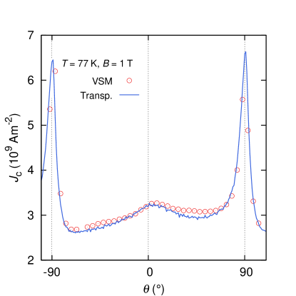
Figure 4: Comparison of magnetisation and transport measurements. The anisotropy measured in the VSM agrees well with transport data, showing a narrow $a,b$-peak and a broad maximum around the $c$-axis, features peculiar to coated conductors. Note the significant asymmetry in both anisotropy curves.

The corresponding experiments were made by performing hysteresis loop measurements at constant angles in the VSM (55 Hz vibration frequency, 0.05–0.15 mm amplitude) sweeping the magnetic field at a rate of $\mu_{0}dH/dt=0.5\,\mathrm{T}/\mathrm{min}$. A 1 µ$\mathrm{V}/\mathrm{cm}$ electric field criterion defined the critical current in the four-probe transport measurements. Both experiments were carried out on the same sample, a YBCO coated conductor grown by MOCVD on a non-magnetic Hastelloy substrate (the single YBCO layer is approximately 1 µm thick). The sample is 4 mm wide and was cut to the optimal length of 22 mm (see Fig. 3) after the transport measurements, which require a slightly longer sample length (about 3 cm) for low-resistance current contacts.

Figure 4 demonstrates that our method agrees very well with transport measurements on the same sample. The two main features of a coated conductor’s anisotropy, a sharp $a$,$b$-peak and a broad $c$-axis maximum, are almost identical. Note, that also the asymmetry of the transport anisotropy curve is reproduced. The magnetisation measurement displayed in Fig. 4 is calibrated against the transport measurement at $\theta=0^{\circ}$. Although the calibration constant differs by only 20 % from the calculated $\alpha^{\star}$, the deviation is significant and will be discussed below.

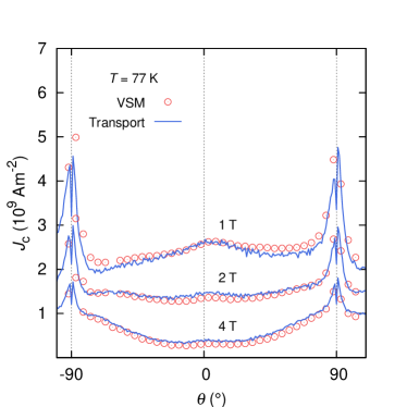
Figure 5: Extrapolation of the transport anisotropy curve to the electric field level of the VSM magnetisation measurement. When measurements at different magnetic fields are compared, the electric field must be considered. Extrapolating the transport $I$-$V$ curves to the low electric fields of a magnetisation measurement leads to satisfactory agreement over a large field range. Note, that the asymmetry observed at 1 T disappears at higher fields.

When comparing measurements at different magnetic fields it is important to take the electric field dependence of the critical current $J_{\mathrm{c}}(E)$ into account, because the $n$-value of the $E(J)=E_{\mathrm{c}}\cdot(J/J_{\mathrm{c}})^{n}$ power-law decreases strongly with increasing magnetic field Thompson et al. (2008). Without accounting for this well-known effect the different electric field levels in both instruments would lead to a magnetic field dependent calibration constant.

A rough estimate of the electric field in the magnetisation measurement is provided by integrating Faraday’s law in a cylindrical coordinate system aligned with the applied magnetic field. The field sweep induces an azimuthal electric field $E_{\mathrm{m}}=r/2\cdot\mu_{0}dH/dt$, which ranges from zero in the centre of the sample to approximately 0.1 – 0.5 µ$\mathrm{V}/\mathrm{cm}$ at the edges of the $22\times 4\,\mathrm{mm}^{2}$ conductor, showing that the average electric field in a magnetisation measurement is significantly below the transport criterion $E_{\mathrm{c,t}}=$1 µ$\mathrm{V}/\mathrm{cm}$. (The indices $t$ and $m$ denote transport and magnetisation in the following.)

We account for the different electric fields by approximating the transport $I$-$V$ curves with a power-law $E_{\mathrm{t}}(J)=E_{\mathrm{c,t}}\cdot(J/J_{\mathrm{c,t}})^{n}$ and extrapolating the transport data to the average electric fields $\bar{E}_{\mathrm{m}}$ of the magnetisation measurements $J_{\mathrm{c,m}}=J_{\mathrm{c,t}}\cdot[E_{\mathrm{t}}/\bar{E}_{\mathrm{m}}\cos(\theta)]^{1/n}$. (The additional factor of $\cos(\theta)$ stems from the angle dependent change of flux trough the sample.) After fitting $\alpha^{\star}$ and $\bar{E}_{\mathrm{m}}$ the measurements compare well over a large field and angular range (see Fig. 5), except, of course, for parallel fields, where $\cos(\theta)=0$ and the electric field breaks down. Satisfactory agreement between transport and magnetisation measurements of the critical current anisotropy in superconducting thin films has, to our knowledge, not been published so far.

The average electric field $\bar{E}_{\mathrm{m}}=0.1$ µ$\mathrm{V}/\mathrm{cm}=E_{\mathrm{t}}/10$, is well within the range of our previous estimation. Taking the electric field into account reduces also the deviation of $\alpha^{\star}$ from theory to below 10 %. The remaining error can be attributed to uncertainties in the superconducting sample dimensions and the fact that especially currents close to the edge of the conductor contribute differently to critical current and magnetic moment.

We wish to emphasise that the low electric field in magnetisation measurements is certainly not a disadvantage. The 1 µ$\mathrm{V}/\mathrm{cm}$-criterion in transport measurements is rather a concession to the voltage noise on short test samples than a technologically relevant criterion—in most applications coated conductors will operate at electric fields much below this criterion. From this perspective, magnetisation experiments are superior, because they are able to explore large critical currents with high resolution down to very low electric fields.

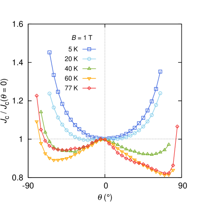
Figure 6: Disappearance of the $c$-axis peak at low temperatures. The $c$-axis peak is observed down to relatively low temperatures (about 20 K at 1 T) and vanishes at 5 K. The curvature of the anisotropy curve at $\theta=0^{\circ}$ thereby changes sign. The increase of the penetration field limits the angular range at low temperatures.

As an example we analyse the temperature dependence of the $c$-axis peak in coated conductors down to temperatures as low as 5 K. This has hitherto been impossible due to the power dissipation in transport measurements and was only recently Xu et al. (2010) achieved at 4.2 K directly in liquid helium. Measurements at 1 T (see Fig. 6) show that the $c$-axis peak vanishes at 5 K. This behaviour is identical to the transport measurements mentioned above, which were carried out on different samples: the anisotropy curve showed a $c$-axis peak at 77 K, but there was no indication of this feature at 4.2 K. The entire temperature dependence, has, to our knowledge, not been reported so far. We are able to monitor the evolution of the $c$-axis peak with our method and find that correlated pinning effects shape the anisotropy down to 20 K at 1 T, but not at lower temperatures.

IV Concluding remarks

The method described in this work is derived for the thin film geometry and may thus be applied not only to coated conductors but to any superconducting thin film of appropriate dimensions. In the case of a magnetic substrate the background signal has to be subtracted, for example, by removing the superconducting layer or by measuring a piece of substrate with identical dimensions. This procedure is, however, only necessary below the saturation field of the magnetic substrate, because according to (3) a reversible background cancels in the evaluation of $J_{\mathrm{c}}$, which depends only on the irreversible magnetic moment.

In general we expect small differences between the magnetic and transport measurements at low applied fields, i.e., when the self-field (roughly 200 mT at 5 K for our sample) of the currents is similar to the applied magnetic field. In this case the direct or indirect (via the magnetic substrate) interaction between the self-field and the field dependent critical currents will differ between transport Sanchez et al. (2010) and magnetisation, because the field profile of the circulating induction currents is different from that of the transport currents. The self-field regime is, however, not important for most applications, which require a detailed knowledge of the critical current anisotropy.

V Summary

We have shown that the critical current anisotropy of a coated conductor at maximum Lorentz force can be measured in a transverse vibrating sample magnetometer. Simply cutting the sample to a defined length eliminates the contribution of spurious variable Lorentz force currents to the magnetic moment sensed by the instrument. The results obtained in this way compare well to transport experiments on the same sample if the effect of the different electric field, which is below the resolution of transport measurements, is accounted for by extrapolating the transport $I$-$V$ curves.

Although the large penetration fields inhibit measurements of the critical current close to the film plane, the advantages of magnetisation measurements, i.e., the lack of current contacts and the low electric field, are obvious. The experiment is thus particularly suited to explore the critical current anisotropy at low magnetic fields and temperatures, which remains inaccessible to transport measurements due to thermal problems.

References

- Thompson et al. (2010) J. R. Thompson, J. W. Sinclair, D. K. Christen, Y. Zhang, Y. L. Zuev, C. Cantoni, Y. Chen, and V. Selvamanickam, Supercond. Sci. Technol. 23, 014002 (2010).
- Mallison (1966) J. Mallison, J. Appl. Phys. 37, 2514 (1966).
- Lacey et al. (1995) D. Lacey, R. Gebauer, and A. D. Caplin, Supercond. Sci. Technol. 8, 568 (1995).
- Mikitik et al. (2004) G. P. Mikitik, E. H. Brandt, and M. Indenbom, Phys. Rev. B 70, 014520 (2004).
- Thompson et al. (2008) J. R. Thompson, Ö. Polat, D. K. Christen, D. Kumar, P. M. Martin, and J. W. Sinclair, Appl. Phys. Lett. 93, 042506 (2008).
- Xu et al. (2010) A. Xu, J. J. Jaroszynski, F. Kametani, Z. Chen, D. C. Larbalestier, Y. L. Viouchkov, Y. Chen, Y. Xie, and V. Selvamanickam, Supercond. Sci. Technol. 23, 014003 (2010).
- Sanchez et al. (2010) A. Sanchez, N. Del-Valle, C. Navau, and D. X. Chen, Appl. Phys. Lett. 97, 072504 (2010).