Recent developments in NLO QCD calculations: the particular case of $pp\rightarrow t\bar{t}jj$

Abstract

A very brief status of next-to-leading order QCD calculations is given. As an example the next-to-leading order QCD calculations to the $pp\to t\bar{t}jj$ processes at the CERN Large Hardon Collider are presented. Results for integrated and differential cross sections are shown. They have been obtained in the framework of the Helac-Nlo system.

1 Introduction

At the CERN Large Hardon Collider we hope to uncover the mechanism of electroweak symmetry breaking and to find signals of physics beyond the Standard Model. Signal events have to be dug out from a bulk of background events, which are due to the Standard Model processes, mostly QCD processes accompanied by additional electroweak bosons. These constitute of final states with a high number of jets or identified particles. LHC data can only be meaningfully analyzed if a plethora of Standard Model background processes are theoretically under control. If one is content with a leading order description of the multijets final states it is possible to go to quite high orders, say 8-10 particles in the final states, which have to be well separated to avoid phase space regions where divergences become troublesome. Quite a number of tools enable one to do this: Alpgen [1], Amegic++/Sherpa [2, 3], Comix/Sherpa [4], CompHEP [5], Helac-Phegas [6, 7, 8], MadGraph/MadEvent [9, 10] and O’mega/Whizard [11]. Those tools, which are based on Feynman diagrams suffer from inefficiency at large n, where n is a number of particles, because the number of diagrams to be evaluated grows rapidly as n increases. Some of the tools above use methods designed to be particularly efficient at high multiplicities. Namely, they build up amplitudes for complex processes using off-shell recursive methods. Nevertheless, all these tools are completely self contained and provide amplitudes and integrators on their own. Although multijet observables can rather easily be modeled at leading order, this description suffers several drawbacks. Leading order calculations depend strongly on the renormalisation scale and can therefore give only an order of magnitude estimate on absolute rates. Besides normalization, sometimes also shapes of distributions are first known at higher orders. Secondly, for many scale processes like e.g. $t\bar{t}H$, $t\bar{t}+nj$, $nj$, $V+nj$, $VV+nj$, where $V$ stands for $W^{\pm}$ and/or $Z$, a proper scale choice is problematic. For some observables dynamical scales seem to work better, for others fixed scales are applied. How do we know which scale to choose ? Moreover, at leading order a jet is modeled by a single parton, which is a very crude approximation. The situation can significantly be improved by including higher order corrections in perturbation theory. Next-to-leading order programs can be divided into three categories. Libraries with a specific list of processes at hadron-hadron colliders like e.g. Mcfm for processes with heavy quarks and/or heavy electroweak bosons, NloJets++ [12] for jet production and Vbfnlo [13] for vector-boson fusion processes. Automatic tools based on Passarino-Veltman [14] reduction of one-loop amplitudes for general $2\to n$ processes like e.g. FeynArts/FormCalc/LoopTools [15, 16] and Golem [17]. And finally, automatic tools based on OPP reduction and other unitarity-based methods, which aim at multiparticle processes at hadron colliders like BlackHat/Sherpa, Rocket/Mcfm and Helac-Nlo. Thanks to all these methods and developments several $2\to 4$ processes have recently been calculated at next-to-leading order QCD, including $pp\to t\bar{t}b\bar{b}$ [18, 19, 20], $pp\to W^{\pm}+3j$ [21, 22, 23, 24, 25], $pp(q\bar{q})\to b\bar{b}b\bar{b}$ [26], $pp\to t\bar{t}jj$ [27], $pp\to Z\gamma^{*}+3j$ [28], $pp\to W^{\pm}W^{\pm}jj$ production via weak-boson fusion [29], QCD-mediated $pp\to W^{+}W^{+}jj$ process [30], and finally $pp\to W^{+}W^{-}b\bar{b}$ [32, 31]. Additionally, the first $2\to 5$ process $pp\to W^{\pm}+4j$ [33] has recently been calculated in the leading-color approximation.

In this contribution, a brief report on the Helac-Nlo approach and the $pp\to t\bar{t}jj$ computation is given.

2 Details of the next-to-leading order calculation

The next-to-leading order results are obtained in the framework of Helac-Nlo based on the Helac-Phegas leading-order event generator for all parton level, which has, on its own, already been extensively used and tested in phenomenological studies see e.g. [34, 35, 36, 37, 38]. The integration over the fractions $x_{1}$ and $x_{2}$ of the initial partons is optimized with the help of Parni [39]. The phase space integration is executed with the help of Kaleu [40] and cross checked with Phegas [7], both general purpose multi-channel phase space generators. The next-to-leading order system consists of:

1. CutTools [41], for the OPP reduction of tensor integrals with a given numerator to a basis of scalar functions and for the rational parts [42, 43, 44];

2. Helac-1Loop [45] for the evaluation of one loop amplitude, more specifically for the evaluation of the numerator functions for given loop momentum (fixed by CutTools);

3. OneLOop [45, 46], a library of scalar functions, which provides the actual numerical values of the integrals.

4. Helac-Dipoles [47], automatic implementation of Catani-Seymour dipole subtraction [48], for the calculation of the real emission part.

Let us emphasize that all parts are calculated fully numerically in a completely automatic manner.

3 Numerical Results

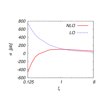
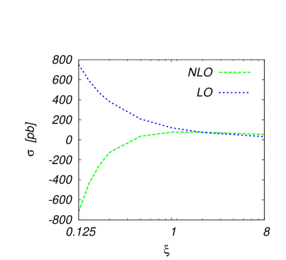
Figure 1: Scale dependence of the total cross section for $pp\rightarrow t\bar{t}jj+X$ at the LHC with $\mu_{R}=\mu_{F}=\xi\cdot m_{t}$. Left panel: The blue dotted curve corresponds to the leading order whereas the red solid to the next-to-leading order one. Right panel: The blue dotted curve corresponds to the leading order whereas the green dashed to the next-to-leading result with a jet veto of 50 GeV.

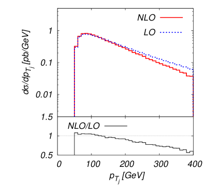
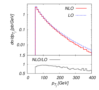
Figure 2: Distribution in the transverse momentum $p_{T_{j}}$ of the $1^{st}$ hardest jet (left panel) and the $2^{nd}$ hardest jet (right panel) for $pp\rightarrow t\bar{t}jj+X$ at the LHC. The blue dotted curve corresponds to the leading order whereas the red solid to the next-to-leading order one.

We consider proton-proton collisions at the LHC with a center of mass energy of $\sqrt{s}=14$ TeV. The mass of the top quark is set to be $m_{t}=172.6$ GeV. We leave it on-shell with unrestricted kinematics. The jets are defined by at most two partons using the $k_{T}$ algorithm [49, 50], with a separation $\Delta R=0.8$, where

$$\Delta R_{ij}=\sqrt{(y_{i}-y_{j})^{2}+(\phi_{i}-\phi_{j})^{2}},~{}~{}~{}~{}~{}~{}y_{i}=1/2\ln\left[(E_{i}-p_{i,z})/(E_{i}+p_{i,z})\right]$$ (1)

being the rapidity and $\phi_{i}$ the azimuthal angle of parton $i$. Moreover, the recombination is only performed if both partons satisfy $|y_{i}|<5$ (approximate detector bounds). We further assume that the jets are separated by $\Delta R=1.0$ and have $|y_{\rm{jet}}|<4.5$. Their transverse momentum is required to be larger than $50$ GeV. We consistently use the CTEQ6 set of parton distribution functions [51, 52], i.e. we take CTEQ6L1 PDFs with a 1-loop running $\alpha_{s}$ in leading order and CTEQ6M PDFs with a 2-loop running $\alpha_{s}$ at next-to-leading order.

We begin our presentation of the final results of our analysis with a discussion of the total cross section. For the central value of the scale, $\mu_{R}=\mu_{F}=m_{t}$, we have obtained:

$$\sigma_{\rm{LO}}=(120.17\pm 0.08)~{}{\rm pb}\,,~{}~{}~{}~{}~{}~{}\sigma_{\rm{NLO}}=(106.95\pm 0.17)~{}{\rm pb}\,.$$ (2)

From the above result one can read a $K$ factor $K=0.89$ which corresponds to the negative corrections of the order of $11\%$.

The scale dependence of the corrections is illustrated in Figure 1. We observe a dramatic reduction of the scale uncertainty while going from leading order to next-to-leading order. Varying the scale up and down by a factor 2 changes the cross section by $+72\%$ and $-39\%$ in the leading order case, while in the next-to-leading order case we have obtained a variation of $-13\%$ and $-12\%$. The third jet, which stems from real radiation, has not been restricted in this case.

Therefore, in the next step, we study the impact of a jet veto on the third jet, which is simply an upper bound on the allowed transverse momentum, $p_{T}$. The total cross section with a jet veto of 50 GeV is

$$\sigma_{\rm{NLO}}(p_{T,X}<50~{}\rm{GeV})=(76.58\pm 0.17)~{}\rm{pb}\;,$$ (3)

which corresponds to $K=0.64$ and negative corrections of the order of $36\%$. In this case a scale variation of $-54\%$ and $-0.3\%$ has been reached, see Figure 1 for graphical representation.

While the size of the corrections to the total cross section is certainly interesting, it is crucial to study the corrections to the distributions. In Figure 2 the transverse momentum distributions of the hardest and second hardest jet are shown for the $pp\rightarrow t\bar{t}jj+X$ process. The blue dashed curve corresponds to the leading order, whereas the red solid one to the next-to-leading order result. The histograms can also be turned into dynamical K-factors, which we display in the lower panels. Distributions demonstrate tiny corrections up to at least 200 GeV, which means that the size of the corrections to the cross section is transmitted to the distributions. On the other hand, strongly altered shapes are visible at high $p_{T}$ especially in case of the first hardest jet. Let us underline here, that corrections to the high $p_{T}$ region can only be correctly described by higher order calculations and are not altered by soft-collinear emissions simulated by parton showers.

4 Summary

We report the results of a next-to-leading order simulation of top quark pair production in association with two jets. With our inclusive cuts, we show that the corrections with respect to leading order are negative and small, reaching $11\%$. The error obtained by scale variation is of the same order.

5 Acknowledgments

I would like to thank the organizers of the International Symposium on Multiparticle Dynamics for the kind invitation and the very pleasant atmosphere during the conference.

The work presented here was funded by the Initiative and Networking Fund of the Helmholtz Association, contract HA-101 (“Physics at the Terascale”) and by the RTN European Programme MRTN-CT-2006-035505 Heptools - Tools and Precision Calculations for Physics Discoveries at Colliders.

References

- [1] M. L. Mangano, M. Moretti, F. Piccinini, R. Pittau, and A. D. Polosa, JHEP 0307, 001 (2003).
- [2] F. Krauss, R. Kuhn, and G. Soff, JHEP 0202, 044 (2002).
- [3] T. Gleisberg et al., JHEP 0902, 007 (2009).
- [4] T. Gleisberg and S. Hoeche, JHEP 0812, 039 (2008).
- [5] A. Pukhov et al., [hep-ph/9908288].
- [6] A. Kanaki and C. G. Papadopoulos, Comput. Phys. Commun. 132, 306 (2000).
- [7] C. G. Papadopoulos, Comput. Phys. Commun. 137, 247 (2001).
- [8] A. Cafarella, C. G. Papadopoulos, and M. Worek, Comput. Phys. Commun. 180, 1941 (2009).
- [9] F. Maltoni and T. Stelzer, JHEP 0302, 027 (2003).
- [10] J. Alwall et al., JHEP 0709, 028 (2007).
- [11] W. Kilian, T. Ohl, and J. Reuter, [arXiv:0708.4233 [hep-ph]].
- [12] Z. Nagy, Phys. Rev. D68, 094002 (2003).
- [13] K. Arnold et al., Comput. Phys. Commun. 180, 1661 (2009).
- [14] G. Passarino and M. J. G. Veltman, Nucl. Phys. B160, 151 (1979).
- [15] T. Hahn and M. Perez-Victoria, Comput. Phys. Commun. 118, 153 (1999).
- [16] T. Hahn, Comput. Phys. Commun. 140, 418 (2001).
- [17] T. Binoth, J. P. Guillet, G. Heinrich, E. Pilon, and T. Reiter, Comput. Phys. Commun. 180, 2317 (2009).
- [18] A. Bredenstein, A. Denner, S. Dittmaier, and S. Pozzorini, Phys. Rev. Lett. 103, 012002 (2009).
- [19] G. Bevilacqua, M. Czakon, C. G. Papadopoulos, R. Pittau, and M. Worek, JHEP 0909, 109 (2009).
- [20] A. Bredenstein, A. Denner, S. Dittmaier, and S. Pozzorini, JHEP 1003, 021 (2010).
- [21] R. K. Ellis, K. Melnikov, and G. Zanderighi, JHEP 0904, 077 (2009).
- [22] C. F. Berger et al., Phys. Rev. Lett. 102, 222001 (2009).
- [23] R. K. Ellis, K. Melnikov, and G. Zanderighi, Phys. Rev. D80, 094002 (2009).
- [24] C. F. Berger et al., Phys. Rev. D80, 074036 (2009).
- [25] K. Melnikov and G. Zanderighi, Phys. Rev. D81, 074025 (2010).
- [26] T. Binoth et al., Phys. Lett. B685, 293 (2010).
- [27] G. Bevilacqua, M. Czakon, C. G. Papadopoulos, and M. Worek, Phys. Rev. Lett. 104, 162002 (2010).
- [28] C. F. Berger et al., Phys. Rev. D82, 074002 (2010).
- [29] B. Jager, C. Oleari, and D. Zeppenfeld, Phys. Rev. D80, 034022 (2009).
- [30] T. Melia, K. Melnikov, R. Rontsch, and G. Zanderighi, JHEP 1012, 053 (2010).
- [31] G. Bevilacqua, M. Czakon, A. van Hameren, C. G. Papadopoulos and M. Worek, [arXiv:1012.4230 [hep-ph].
- [32] A. Denner, S. Dittmaier, S. Kallweit and S. Pozzorini, [arXiv:1012.3975 [hep-ph]].
- [33] C. F. Berger et al., [arXiv:1009.2338 [hep-ph]].
- [34] T. Gleisberg et al., Eur. Phys. J. C34, 173 (2004).
- [35] C. G. Papadopoulos and M. Worek, Eur. Phys. J. C50, 843 (2007).
- [36] J. Alwall et al., Eur. Phys. J. C53, 473 (2008).
- [37] C. Englert, B. Jager, M. Worek, and D. Zeppenfeld, Phys. Rev. D80, 035027 (2009).
- [38] S. Actis et al., Eur. Phys. J. C66, 585 (2010).
- [39] A. van Hameren, Acta Phys. Polon. B40, 259 (2009).
- [40] A. van Hameren, [arXiv:1003.4953 [hep-ph]].
- [41] G. Ossola, C. G. Papadopoulos, and R. Pittau, JHEP 0803, 042 (2008).
- [42] G. Ossola, C. G. Papadopoulos, and R. Pittau, Nucl. Phys. B763, 147 (2007).
- [43] G. Ossola, C. G. Papadopoulos, and R. Pittau, JHEP 0805, 004 (2008).
- [44] P. Draggiotis, M. V. Garzelli, C. G. Papadopoulos, and R. Pittau, JHEP 0904, 072 (2009).
- [45] A. van Hameren, C. G. Papadopoulos, and R. Pittau, JHEP 0909, 106 (2009).
- [46] A. van Hameren, [arXiv:1007.4716 [hep-ph]].
- [47] M. Czakon, C. G. Papadopoulos, and M. Worek, JHEP 0908, 085 (2009).
- [48] S. Catani, S. Dittmaier, M. H. Seymour, and Z. Trocsanyi, Nucl. Phys. B627, 189 (2002).
- [49] S. Catani, Y. L. Dokshitzer, and B. R. Webber, Phys. Lett. B285, 291 (1992).
- [50] S. Catani, Y. L. Dokshitzer, M. H. Seymour, and B. R. Webber, Nucl. Phys. B406, 187 (1993).
- [51] J. Pumplin et al., JHEP 0207, 012 (2002).
- [52] D. Stump et al., JHEP 0310, 046 (2003).