The thermodynamic Casimir force: A Monte Carlo study of the crossover between the ordinary and the normal surface universality class

Abstract

We study the crossover from the ordinary to the normal surface universality class in the three-dimensional Ising bulk universality class. This crossover is relevant for the behavior of films of binary mixtures near the demixing point and a weak adsorption at one or both surfaces. We perform Monte Carlo simulations of the improved Blume-Capel model on the simple cubic lattice. We consider systems with film geometry, where various boundary conditions are applied. We discuss corrections to scaling that are caused by the surfaces and their relation with the so called extrapolation length. To this end we analyze the behavior of the magnetization profile near the surfaces of films. We obtain an accurate estimate of the renormalization group exponent $y_{h_{1}}=0.7249(6)$ for the ordinary surface universality class. Next we study the thermodynamic Casimir force in the crossover region from the ordinary to the normal surface universality class. To this end, we compute the Taylor-expansion of the crossover finite size scaling function up to the second order in $h_{1}$ around $h_{1}=0$, where $h_{1}$ is the external field at one of the surfaces. We check the range of applicability of the Taylor-expansion by simulating at finite values of $h_{1}$. Finally we study the approach to the strong adsorption limit $h_{1}\rightarrow\infty$. Our results confirm the qualitative picture that emerges from exact calculations for stripes of the two-dimensional Ising model, [D. B. Abraham and A. Maciołek, Phys. Rev. Lett. 105, 055701 (2010)], mean-field calculations and preliminary Monte Carlo simulations of the Ising model on the simple cubic lattice, [T. F. Mohry et al, Phys. Rev. E 81, 061117 (2010)]: For certain choices of $h_{1}$ and the thickness of the film, the thermodynamic Casimir force changes sign as a function of the temperature and for certain choices of the temperature and $h_{1}$, it also changes sign as a function of the thickness of the film.

I Introduction

In 1978 Fisher and de Gennes FiGe78 realized that when thermal fluctuations are restricted by a container, a force acts on its walls. Since this effect is analogous to the Casimir effect Casimir , where the restriction of quantum fluctuations induces a force, it is called “thermodynamic” Casimir effect. Since thermal fluctuations only extend to large scales in the neighborhood of continuous phase transitions it is also called “critical” Casimir effect. Recently this force could be detected for various experimental systems and quantitative predictions could be obtained from Monte Carlo simulations of spin models Ga09 .

The behavior of the thermodynamic Casimir force can be described by finite size scaling (FSS) Barber laws. For the film geometry that we consider here, one gets Krech for the thermodynamic Casimir force per area

$$F_{Casimir}\simeq k_{B}TL_{0}^{-3}\;\theta_{(UC_{1},UC_{2})}(t[L_{0}/\xi_{0}]^{1/\nu})$$ (1)

where $L_{0}$ is the thickness of the film and $t=(T-T_{c})/T_{c}$ is the reduced temperature and $T_{c}$ the critical temperature. Note that below, analyzing our data, we shall use for simplicity the definition $t=\beta_{c}-\beta$, where $\beta=1/k_{B}T$. The amplitude $\xi_{0}$ of the correlation length $\xi$ is defined by

$$\xi=\xi_{0,\pm}|t|^{-\nu}\times(1+a_{\pm}|t|^{\nu\omega}+ct+...)$$ (2)

where $-$ and $+$ indicate the high and the low temperature phase, respectively. Since the correlation length can be determined more accurately in the high temperature phase than in the low temperature phase, we take $\xi_{0}=\xi_{0,+}$ in eq. (1). The power law (2) is subject to confluent corrections, such as $a_{\pm}|t|^{\nu\omega}$, and non-confluent ones such as $ct$. Critical exponents such as $\nu$ and ratios of amplitudes such as $\xi_{0,+}/\xi_{0,-}$ are universal. Also correction exponents such as $\omega$ and ratios of correction amplitudes such as $a_{+}/a_{-}$ are universal. For the three-dimensional Ising universality class, which is considered here $\nu\omega\approx 0.5$. For reviews on critical phenomena and their modern theory, i.e., the Renormalization Group (RG) see, e.g., WiKo ; Fisher74 ; Fisher98 ; PeVi02 . The universal finite size scaling function $\theta_{(UC_{1},UC_{2})}$ depends on the universality class of the bulk system as well as the surface universality classes $UC_{1}$ and $UC_{2}$ of the two surfaces of the film. For reviews on surface critical phenomena see e.g. BinderS ; Diehl86 ; Diehl97 . We shall give a brief discussion below in section III.

In the past few years there has been great interest in the crossover behaviors of the thermodynamic Casimir force. In ScDi08 the authors have studied the crossover from the special surface universality class to the ordinary one by using field theoretic methods. They find that for certain choices of the parameters, the thermodynamic Casimir force changes sign with a varying thickness of the film. The authors of AbMa09 have computed exactly the thermodynamic Casimir force for stripes of the two-dimensional Ising model as a function of the external surface fields $h_{1}$ and $h_{2}$. Also here the authors have found that for certain choices of the fields $h_{1}$ and $h_{2}$, the thermodynamic Casimir force does change sign as a function of the temperature or the thickness of the film. More recently, the authors of MoMaDi10 have studied the crossover from the ordinary to the normal surface universality class, and the crossover from the special to the ordinary as well as the normal surface universality class using the mean-field approximation. Also in these cases a change of sign of the thermodynamic Casimir force could be observed. Furthermore in MoMaDi10 preliminary results Va of Monte Carlo simulations of the spin-1/2 Ising model on the simple cubic lattice for the crossover from the ordinary to the normal surface universality class were presented. Following the authors of MoMaDi10 these observations might be of technological relevance. They write: ”Such a tunability of critical Casimir forces towards repulsion might be relevant for micro- and nano-electromechanical systems in order to prevent stiction due to the omnipresent attractive quantum mechanical Casimir forces Casimir ; Ball .” In recent experiments on colloidal particles immersed in a binary mixture of fluids NeHeBe09 , the authors have demonstrated that the adsorption strength can be varied continuously by a chemical modification of the surfaces. In particular the situation of effectively equal adsorption strengths for the two fluids can be reached. For sufficiently small ordering interaction at the surface, this corresponds to the ordinary surface universality class. Hence these experiments open the way to study the crossover from the ordinary to the normal universality class. As discussed in refs. PAT1 ; PAT2 ; PAT3 ; PAT4 effectively weak adsorption can also be obtained by using patterned substrates.

In the present work we compute scaling functions for the film or plate-plate geometry. In order to compare with experiments on the thermodynamic Casimir force between colloidal particles and a flat substrate as studied in ref. NeHeBe09 the scaling function for the plate-sphere geometry has to be computed. The Derjaguin approximation De34 might be used to derive scaling functions for the plate-sphere geometry from those for the plate-plate geometry if the radius of the sphere is large compared with the distance between the plate and the sphere HaScEiDi98 ; ScHaDi03 , as it is indeed the case in ref. NeHeBe09 . In the recent works Nature08 ; Gaetal09 the Derjaguin approximation had been used to obtain the scaling functions for the plate-sphere geometry in the strong adsorption limit starting from the Monte Carlo estimates of refs. VaGaMaDi07 ; VaGaMaDi08 for the film geometry.

As in ref. myCasimir , where we had studied the strong adsorption limit, we shall study the crossover by performing Monte Carlo simulations of the improved Blume-Capel model on the simple cubic lattice. We shall give the definition of this model in section II below. Improved means that corrections to finite size scaling that are $\propto L_{0}^{-\omega}$ vanish. This property is very useful in the study of films, since typically the surfaces cause corrections $\propto L_{0}^{-1}$ BinderS ; Diehl86 ; Diehl97 and fitting Monte Carlo data, it is quite difficult to disentangle corrections that have similar exponents. Motivated by the experiments NeHeBe09 , we shall mainly study films where the external field $h_{1}$ at the first surface is finite, while at the other surface the limit $h_{2}\rightarrow\infty$ is taken, corresponding to the strong adsorption limit in a binary mixture. For this choice of boundary conditions the correlation length of the film divided by its thickness remains small at any temperature. In contrast, for $h_{1}=h_{2}=0$ the film undergoes a second order phase transition in the universality class of the two-dimensional Ising model. This implies that in the neighborhood of this transition the correlation length of the film divided by its thickness is large. Therefore the Monte Carlo study of the crossover from $h_{1}=h_{2}=0$ to the limit $|h_{1}|,|h_{2}|\rightarrow\infty$ would be more involved than that performed here.

In preparation for our study of the thermodynamic Casimir force, we have accurately determined the surface critical exponent $y_{h_{1}}$ of the ordinary surface universality class. Furthermore we have estimated the so called extrapolation length for various boundary conditions. The extrapolation length is directly related to the corrections to finite size scaling that are caused by the surfaces of the film. Our numerical results are mainly based on the analysis of the behavior of the magnetization profile at the bulk critical temperature. Next we have computed the thermodynamic Casimir force for the range of inverse temperatures around the bulk critical point where, at the level of our numerical accuracy, it is non-vanishing. To this end we follow the suggestion of Hucht Hucht . For alternative methods see KrLa95 ; VaGaMaDi07 ; VaGaMaDi08 ; yet . Note that the stress tensor method of DaKr04 can only be applied for periodic or anti-periodic boundary conditions. First we have simulated films with a vanishing surface field $h_{1}=0$. Based on the data obtained from these simulations, we have also computed the Taylor-expansion of the thermodynamic Casimir force per area in $h_{1}$ up to the second order around $h_{1}=0$. We demonstrate that, taking into account corrections $\propto L_{0}^{-1}$, already for the relatively small thicknesses $L_{0}=8.5$, $12.5$, and $16.5$ the behavior of the thermodynamic Casimir force per area as well as its partial derivatives with respect to $h_{1}$ is well described by universal FSS functions. Next we have simulated films with various finite values of $h_{1}$ to check the range of applicability of the Taylor-expansion and to study the crossover beyond this range. Finally we have studied the approach to the strong adsorption limit $h_{1}\rightarrow\infty$. Qualitatively we confirm the picture that emerges from the exact solution of the two-dimensional Ising model AbMa09 and the mean-field calculation MoMaDi10 .

The outline of the paper is the following: In section II we define the model and the observables that we have studied. In section III we briefly review the phase diagram of a semi-infinite system. Then in section IV we discuss the finite size scaling behavior of the magnetization profile at the bulk critical point and the finite size scaling behavior of the thermodynamic Casimir force. In section V we discuss how to compute the thermodynamic Casimir force and its partial derivatives with respect to the external field $h_{1}$ at the surface. In section VI we present the results of our Monte Carlo simulations. We performed a series of simulations at the bulk critical point, where we focus on the magnetization profile. Next we have determined the thermodynamic Casimir force per area in the neighborhood of the bulk critical point for various values of the external field $h_{1}$ at the surface. Finally, in section VII we summarize and conclude.

II The model and bulk observables

We study the Blume-Capel model on the simple cubic lattice. It is characterized by the reduced Hamiltonian

$$H=-\beta\sum_{<xy>}s_{x}s_{y}+D\sum_{x}s_{x}^{2}-h\sum_{x}s_{x}$$ (3)

where $x=(x_{0},x_{1},x_{2})$ denotes a site of the lattice. The components $x_{0}$ ,$x_{1}$ and $x_{2}$ take integer values. The spin $s_{x}$ might take the values $-1$, $0$ or $1$. In the following we shall consider a vanishing external field $h=0$ throughout. The parameter $D$ controls the density of vacancies $s_{x}=0$. In the limit $D\rightarrow-\infty$ the spin-1/2 Ising model is recovered. For $-\infty\leq D<D_{tri}$ the model undergoes a second order phase transition in the three-dimensional Ising universality class. For $D>D_{tri}$ the transition is of first order. The most recent estimate for the tri-critical point is $D_{tri}=2.0313(4)$ DeBl04 . Numerically, using Monte Carlo simulations it has been shown that there is a point $(D^{*},\beta_{c}(D^{*}))$ on the line of second order phase transitions, where the amplitude of leading corrections to scaling vanishes. Our most recent estimate is $D^{*}=0.656(20)$ mycritical . In mycritical we have simulated the model at $D=0.655$ close to $\beta_{c}$ on lattices of a linear size up to $L=360$. From a standard finite size scaling analysis of phenomenological couplings such as the Binder cumulant we find

$$\beta_{c}(0.655)=0.387721735(25)$$ (4)

for the inverse of the critical temperature at $D=0.655$. The amplitude of leading corrections to scaling at $D=0.655$ is at least by a factor of $30$ smaller than for the spin-1/2 Ising model.

Our recent estimates for bulk critical exponents in the three-dimensional Ising universality class are mycritical

$$\nu = 0.63002(10)\;\;,$$ (5)

$$\eta = 0.03627(10)\;\;,$$ (6)

$$\omega = 0.832(6)\;\;.$$ (7)

In the following we set the scale by using the second moment correlation length $\xi_{2nd}$ in the high temperature phase of the model. On a finite lattice of the linear size $L$ in each of the directions it might be defined by

$$\xi_{2nd}=\sqrt{\frac{\chi/F-1}{4\sin^{2}\pi/L}}$$ (8)

where

$$F=\frac{1}{L^{3}}\left\langle\Big{|}\sum_{x}\exp\left(i\frac{2\pi x_{k}}{L}\right)s_{x}\Big{|}^{2}\right\rangle$$ (9)

is the Fourier transform of the correlation function at the lowest non-zero momentum and

$$\chi=\frac{1}{L^{3}}\left\langle\Big{(}\sum_{x}s_{x}\Big{)}^{2}\right\rangle$$ (10)

is the magnetic susceptibility. In myamplitude ; myCasimir we find

$$\xi_{2nd,0,+}=0.2282(2)-1.8\times(\nu-0.63002)+250\times(\beta_{c}-0.387721735)$$ (11)

for the amplitude of the second moment correlation length in the high temperature phase, where we have used

$$t=\beta_{c}-\beta$$ (12)

as definition of the reduced temperature. We shall use this definition of $t$ also in the following. The energy density is defined by

$$E_{bulk}=\frac{1}{L^{3}}\sum_{<xy>}\langle s_{x}s_{y}\rangle\;\;.$$ (13)

In the following we shall need the energy density of the bulk system in a neighborhood of the bulk critical point. To this end, we have performed simulations at 350 different values of $\beta$ in the range $0.25\leq\beta\leq 0.6$ myamplitude . In a small neighborhood of $\beta_{c}$, where no direct simulations are available we use

$$E_{bulk}(\beta)=E_{ns}+C_{ns}(\beta-\beta_{c})+a_{\pm}|\beta-\beta_{c}|^{1-\alpha}+d_{ns}(\beta-\beta_{c})^{2}+b_{\pm}|\beta-\beta_{c}|^{2-\alpha}\;\;.$$ (14)

For a discussion see section IV of myamplitude .

II.1 Film geometry and boundary conditions

Here we study systems with a film geometry. In the ideal case this means that the system has a finite thickness $L_{0}$, while in the other two directions the thermodynamic limit $L_{1},L_{2}\rightarrow\infty$ is taken. In our Monte Carlo simulations we shall study lattices with $L_{0}\ll L_{1}=L_{2}=L$ and apply periodic boundary conditions in the $1$ and $2$ directions.

The reduced Hamiltonian of the Blume-Capel model with film geometry is

$$H = -\beta\sum_{<xy>}s_{x}s_{y}+D\sum_{x}s_{x}^{2}$$

$$- \beta_{1}\sum_{<xy>,x_{0}=y_{0}=1}s_{x}s_{y}\;-\;\beta_{2}\sum_{<xy>,x_{0}=y_{0}=L_{0}}s_{x}s_{y}\;-\;h_{1}\sum_{x,x_{0}=1}s_{x}\;-\;h_{2}\sum_{x,x_{0}=L_{0}}s_{x}$$

where $h_{1},h_{2}\neq 0$ break the symmetry at the surfaces that are located at $x_{0}=1$ and $x_{0}=L_{0}$, respectively. In our convention $<xy>$ runs over all pairs of nearest neighbor sites with fluctuating spins. Note that here the sites $(1,x_{1},x_{2})$ and $(L_{0},x_{1},x_{2})$ are not nearest neighbors as it would be the case for periodic boundary conditions. In our study, we set $\beta_{1}=\beta_{2}=0$ throughout. Hence there is no enhancement of the coupling at the surface. There is ambiguity, where one puts the boundaries and how the thickness of the film is precisely defined. Here we follow the convention that $L_{0}$ gives the number of layers with fluctuating spins. In our previous work myCasimir we have studied the limit of strong adsorption, $|h_{1}|,|h_{2}|\rightarrow\infty$. In this limit the spins at the boundary are fixed to either $-1$ or $+1$. Therefore we had put the fixed spins on $x_{0}=0$ and $x_{0}=L_{0}+1$ to get $L_{0}$ layers with fluctuating spins. Note that these fixed spins could also be interpreted as external fields $h_{1,2}=\pm\beta$ acting on the spins at $x_{0}=1$ and $x_{0}=L_{0}$, respectively. In the following we shall denote the type of boundary conditions by $(h_{1},h_{2})$. In the literature the cases $h_{1}=0$ or $h_{2}=0$ are often called free boundary conditions. To be consistent with the literature, we shall denote the strong adsorption limit by $+$ or $-$ in the following. In particular the two cases studied in myCasimir are denoted by $(+,+)\equiv(\beta,\beta)$ and $(+,-)\equiv(\beta,-\beta)$. For the discussion of the behavior of physical quantities near the boundary it is useful to define the distance from the boundary. To this end we shall assume that the first boundary is located at $x_{0}=1/2$ and the second one at $x_{0}=L_{0}+1/2$. Hence the distance from the first boundary is given by $z=x_{0}-1/2$ and the distance from the second one by $z=-x_{0}+L_{0}+1/2$.

In order to determine the thermodynamic Casimir force we have measured the energy per area of the film. It is given by

$$E=\frac{1}{L^{2}}\left\langle\sum_{<xy>}s_{x}s_{y}\right\rangle\;\;.$$ (16)

Since the film is invariant under translations in $1$ and $2$ directions but not in $0$ direction, the magnetization depends on $x_{0}$. Therefore we define the magnetization of a slice by

$$m(x_{0})=\frac{1}{L^{2}}\left\langle\sum_{x_{1},x_{2}}s_{x}\right\rangle\;.$$ (17)

III Phase diagram of a semi-infinite system

Here we briefly recall the phase diagram of a semi-infinite Ising system as it is discussed e.g. in the reviews BinderS ; Diehl86 ; Diehl97 . For the Blume-Capel model, we expect that for $D\lessapprox 2$ the qualitative features of the phase diagram remain unchanged since $D_{tri}=1.966(2)$ SiCaPl06 for the two-dimensional system and $D_{tri}=2.0313(4)$ DeBl04 for the three-dimensional one.

In figure 1 we have sketched the phase diagram for a vanishing external field $h=0$ and a vanishing surface field $h_{1}=0$. For $\beta>\beta_{c}$ the spins in the bulk are ordered. As a consequence, also the spins at the surface are ordered. This phase is denoted by C in figure 1. At vanishing bulk coupling $\beta=0$ the spins at the surface decouple completely from those of the bulk. Hence a two dimensional Ising or Blume-Capel model remains that undergoes a phase transition at $\beta_{1}=\beta_{c,2D}$. Starting from the point $(0,\beta_{c,2D})$ there is a line of transitions, where the spins at the surface order, while those of the bulk remain disordered. This line hits the vertical line at $\beta=\beta_{c}$ in the so called special or surface-bulk point that we denote by SB in figure 1, which is a tri-critical point. In figure 1, the phase, where both the boundary spins and those of the bulk are disordered is denoted by A while the one with disordered bulk and ordered surface is denoted by B. The transitions from phase A to phase C are so called ordinary transitions, while those from phase B to phase C are so called extraordinary transitions. The transitions from phase A to B are so called surface transitions.

Figure 1: Sketch of the phase diagram of the semi-infinite system. On the $x$-axis we plot the coupling $\beta$ of the bulk and on the $y$-axis the excess coupling $\beta_{1}$ of the surface. A detailed discussion is given in the text.

For $h_{1}\neq 0$ the spins at the surface are ordered also for $\beta_{1}\leq\beta_{1,s}$. In the literature the transitions from disordered to ordered spins in the bulk for $h_{1}\neq 0$ are called normal transitions. In BuDi94 it has been shown that the normal surface universality class is equivalent to the extraordinary surface universality class.

At the ordinary transition the external field $h_{1}$ at the surface is a relevant perturbation. Hence the RG-exponent $y_{h_{1}}$ associated with the surface field is positive. In the literature, a number of surface critical exponents have been introduced. In the case of the ordinary transition, these can be obtained from $y_{h_{1}}$ and the bulk RG-exponents $y_{t}=1/\nu$ and $y_{h}=(d+2-\eta)/2$ by using scaling relations. In the following we need

$$\Delta_{1} = \nu y_{h_{1}}\;\;,$$ (18)

$$\beta_{1} = \nu(d-1-y_{h_{1}})\;\;,$$ (19)

$$\gamma_{1} = \nu(2-d/2-\eta/2+y_{h_{1}})\;\;.$$ (20)

For the definitions and a complete list of these exponents see the reviews BinderS ; Diehl86 ; Diehl97 . The numerical values of surface critical exponents for the three-dimensional Ising universality class have been computed by various theoretical methods. Mean field theory predicts $y_{h_{1}}=1/2$. The authors of BuEi78 quote $y_{h_{1}}=0.7363$ as result of their real space RG method and the authors of WhToGu79 quote $\gamma_{1}=0.78(2)$ as result of a series expansion, which corresponds to $y_{h_{1}}=0.72(3)$. The $\epsilon$-expansion gives DiDi81

$$y_{h_{1}}=\frac{1}{2}+\frac{1}{6}\epsilon+\frac{31}{321}\epsilon^{2}+O(\epsilon^{3})\;\;.$$ (21)

Naively inserting $\epsilon=1$ one gets $y_{h_{1}}=0.666...$ and $y_{h_{1}}=0.762...$ at $O(\epsilon)$ and $O(\epsilon^{2})$, respectively. Using a massive field theory approach the authors of DiSh98 obtain $\Delta_{1}=0.45$ from the $[1/1]$ Padé approximant of their two-loop result, which corresponds to $y_{h_{1}}=0.714$. Comparing the different Padé approximants that are given in table 9 of DiSh98 one might conclude that the uncertainty of the estimate of $y_{h_{1}}$ is about $0.02$. In table 1 we have summarized Monte Carlo results for surface critical exponents. Most of the authors quote an estimate for $\beta_{1}$ and some in addition for $\gamma_{1}$. In those cases in which the authors did not quote a result for $y_{h_{1}}$ we have converted the value given for $\beta_{1}$ using the scaling relation (19) and $\nu=0.63002(10)$.

Table 1: Monte Carlo results for surface critical exponents for the ordinary phase transition in the three-dimensional Ising universality class. The authors of KiOk85 quote no final result for $\gamma_{1}$. Here we give the average of the three results given in table II of KiOk85 . In case the authors do not quote an estimate for $y_{h_{1}}$, we have computed it from $\beta_{1}$ and the scaling relation (19). These cases are marked by ^∗.

Ref.	$\beta_{1}$	$\gamma_{1}$	$y_{h_{1}}$
BiLa84	0.78(2)		0.762(32)∗
KiOk85	0.79(2)	0.79(10)	0.746(32)∗
LaBi90	0.78(2)	0.78(6)	0.762(32)∗
NiBl93			0.740(15)
RuWa95	0.807(4)	0.760(4)	0.719(6)∗
PlSe98	0.80(1)	0.78(5)	0.730(16)∗
DeBl03			0.737(5)
DeBlNi05	0.796(1)		0.7374(15)
LiZh08	0.795(6)		0.738(10)∗
here			0.7249(6)

For comparison we also anticipate our result for $y_{h_{1}}$ that we obtain in section VI.1 below. Except for RuWa95 the estimates for $y_{h_{1}}$ are larger than ours. In particular, note that the difference between our result and that of DeBlNi05 is about six times as large as the combined error.

IV Finite size scaling applied to films

In this section we shall discuss the finite size scaling behavior of the magnetization profile at the bulk critical point and thermodynamic Casimir force for arbitrary temperature. The starting point of our considerations is the reduced excess free energy per area of the film

$$f_{ex}(L_{0},t,h_{1})=f_{film}(L_{0},t,h_{1})-L_{0}f_{bulk}(t)$$ (22)

where $f_{film}(L_{0},t,h_{1})$ is the reduced free energy of the film per area and $f_{bulk}(t)$ the reduced bulk free energy density. There is no dependence on $h_{2}$, since we consider the limit $h_{2}\rightarrow\infty$. The singular part of the reduced excess free energy per area has the finite size scaling behavior BinderS ; Diehl86 ; Diehl97

$$f_{ex,s}(L_{0},t,h_{1})=L_{0}^{-d+1}g(t[L_{0}/\xi_{0}]^{y_{t}},h_{1}[L_{0}/l_{ex,nor,0}]^{y_{h_{1}}})$$ (23)

where we have ignored corrections to scaling at the moment and $d=3$ is the dimension of the bulk system. We shall define the amplitude $l_{ex,nor,0}$ of the normal extrapolation length $l_{ex,nor}$ below, eq. (30). Note that the bulk contributions to the non-singular part of the free energy cancel in eq. (22). However, there remain contributions from the two surfaces.

IV.1 The magnetization profile at the bulk critical point

In terms of the reduced free energy per area the magnetization at $x_{0}=1$ is given by

$$m_{1} = \frac{\partial f_{ex}(L_{0},t,h_{1})}{\partial h_{1}}$$ (24)

$$= \frac{1}{L^{2}}\;\frac{1}{Z}\frac{\sum_{\{s\}}\exp(...+h_{1}\sum_{x_{1},x_{2}}s_{(1,x_{1},x_{2})})}{\partial h_{1}}=\frac{1}{L^{2}}\left\langle\sum_{x_{1},x_{2}}s_{(1,x_{1},x_{2})}\right\rangle\;\;.$$

In section VI.1 we shall determine the value of the RG-exponent $y_{h_{1}}$ from the scaling of $m_{1}$ with the thickness $L_{0}$ at $h_{1}=0$ and $\beta=\beta_{c}$. Taking the partial derivative of eq. (23) with respect to $h_{1}$ we get

$$m_{1} = \left.\frac{\partial f_{ex}}{\partial h_{1}}\right|_{t=h_{1}=0}=L_{0}^{-d+1}\left.\frac{\partial g(t[L_{0}/\xi_{0}]^{y_{t}},h_{1}[L_{0}/l_{ex,nor,0}]^{y_{h_{1}}})}{\partial h_{1}}\right|_{t=h_{1}=0}$$ (25)

$$= L_{0}^{-d+1}\left.g_{h_{1}}(0,0)\right|_{t=h_{1}=0}[L_{0}/l_{ex,nor,0}]^{y_{h_{1}}}=c\,L_{0}^{-d+1+y_{h_{1}}}$$

where $g_{h_{1}}$ denotes the partial derivative of $g$ with respect to $x_{h_{1}}=h_{1}[L_{0}/l_{ex,nor,0}]^{y_{h_{1}}}$. Note that the non-singular contribution to $f_{ex}$ from the first surface does not feel the breaking of the symmetry by the second surface. Therefore it is an even function of $h_{1}$ and does not contribute to the partial derivative with respect to $h_{1}$.

The extrapolation length $l_{ex}$ can be defined by the behavior BinderS ; Diehl86 ; Diehl97

$$m(x_{0})=c\,L_{0}^{-\beta/\nu}\;\psi(x_{0}/L_{0})$$ (26)

of the magnetization profile at the critical point of the bulk system. Note that from scaling relations it follows that $\beta/\nu=(1+\eta)/2$, where $\eta=0.03627(10)$ for the three-dimensional Ising universality class mycritical .

In the neighborhood of the surface with spins fixed to $s_{x}=1$, one expects that for $z\ll L_{0}$, where $z=L_{0}-x_{0}+1/2$, the magnetization profile does not depend on $L_{0}$. Therefore $\psi(x_{0}/L_{0})=(z/L_{0})^{-\beta/\nu}$ and hence BinderS ; Diehl86 ; Diehl97

$$m(x_{0})=c\,z^{-\beta/\nu}\;.$$ (27)

Also at the free boundary we expect that for $z\ll L_{0}$, where now $z=x_{0}-1/2$, the functional form of the magnetization profile does not depend on $L_{0}$. As we have seen above, for a fixed value of $z$, the magnetization behaves as $m_{1}\propto L_{0}^{-d+1+y_{h_{1}}}$. Therefore BinderS ; Diehl86 ; Diehl97

$$m(x_{0})=a\,z^{-\beta/\nu+d-1-y_{h_{1}}}=a\,z^{(\beta_{1}-\beta)/\nu}\;\;.$$ (28)

Since $-\beta/\nu<0$, the scaling function of the magnetization profile diverges as $z/L_{0}\rightarrow 0$ at the boundary with fixed spins. On the other hand since $(\beta_{1}-\beta)/\nu>0$ the scaling function of the magnetization vanishes as $z/L_{0}\rightarrow 0$ at the free boundary.

Based on this observation one might define for finite thicknesses $L_{0}$ an effective distance from the boundary

$$z_{eff}=z+l_{ex}$$ (29)

such that the magnetization profile at $z_{eff}=0$ vanishes for $h_{1}=0$ or diverges in the case of symmetry breaking boundary conditions. The concept of the extrapolation length has been worked out explicitly for the ordinary transition in the framework of mean-field theory BinderS . Also in the Monte Carlo study of the magnetization profile of a semi-infinite system in the extraordinary surface universality class an extrapolation length had been introduced SmDiLa94 . The extrapolation length is related with corrections $\propto L_{0}^{-1}$ discussed in the framework of field-theory in DiDiEi83 . In the following we shall distinguish between the extrapolation length $l_{ex,ord}$ ($ord$ for ordinary surface transition) and $l_{ex,nor}$ ($nor$ for normal surface transition) in the case of symmetry breaking boundary conditions. The extrapolation length depends on the precise definition of $z$. Physically, the extrapolation length depends on the details of the microscopic model, in particular on the details of the fields and interactions at the surface. In section VI.2 we shall study the behavior of the extrapolation length as a function of the field $h_{1}$ at the boundary. One expects BrLei8283

$$l_{ex,nor}(h_{1})=l_{ex,nor,0}\,h_{1}^{-1/y_{h_{1}}}$$ (30)

which defines the amplitude $l_{ex,nor,0}$ that we have already used above in eq. (23).

Capehart and Fisher CaFi76 have argued that the arbitrariness in the definition of the thickness of the film leads to corrections $\propto L_{0}^{-1}$. These corrections can be eliminated by replacing $L_{0}$ in finite size scaling laws such as eq. (23) by an effective thickness

$$L_{0,eff}=L_{0}+L_{s}$$ (31)

of the film. Assuming that the corrections due to a surface are caused by a unique irrelevant surface scaling field, the constant $L_{s}$ should be given by

$$L_{s}=l_{ex,1}+l_{ex,2}$$ (32)

where $l_{ex,1}$ and $l_{ex,2}$ are the extrapolation lengths at the two surfaces of the film. In section II A 4 of ref. Gaetal09 a similar discussion of the extrapolation length had been presented. For a discussion of the effective thickness and further references see section IV of ref. myCasimir .

IV.2 Crossover scaling function of the thermodynamic Casimir force

In terms of the reduced excess free energy per area the thermodynamic Casimir force per area is given by Krech

$$\frac{1}{k_{B}T}F_{Casimir}=-\frac{\partial f_{ex}}{\partial L_{0}}\;\;.$$ (33)

Using the finite size scaling law (23) we arrive at

$$\frac{\partial f_{ex,s}(L_{0},t,h_{1})}{\partial L_{0}} = (-d+1)L_{0}^{-d}g(x_{t},x_{h_{1}})+L_{0}^{-d}y_{t}t[L_{0}/\xi_{0}]^{y_{t}}\;g_{t}(x_{t},x_{h})$$ (34)

$$+ L_{0}^{-d}y_{h1}h_{1}[L_{0}/l_{ex,nor,0}]^{y_{h1}}g_{h_{1}}(x_{t},x_{h_{1}})$$

where $x_{t}=t[L_{0}/\xi_{0}]^{y_{t}}$ and $x_{h_{1}}=h_{1}[L_{0}/l_{ex,nor,0}]^{y_{h1}}$. The partial derivatives of $g$ with respect to $x_{t}$ and $x_{h_{1}}$ are denoted by $g_{t}$ and $g_{h_{1}}$, respectively. Note that the analytic part of $f_{ex}$ is due to the surfaces and does not depend on $L_{0}$ and therefore does not contribute to the thermodynamic Casimir force. It follows that the thermodynamic Casimir force per area follows the finite size scaling law MoMaDi10

$$F_{Casimir}=k_{B}TL_{0}^{-d}\Theta(t[L_{0}/\xi_{0}]^{y_{t}},h_{1}[L_{0}/l_{ex,nor,0}]^{y_{h1}})$$ (35)

where

$$\Theta(x_{t},x_{h_{1}})=(d-1)g(x_{t},x_{h_{1}})-y_{t}t[L_{0}/\xi_{0}]^{y_{t}}\;g_{t}(x_{t},x_{h})-y_{h1}h_{1}[L_{0}/l_{ex,nor,0}]^{y_{h1}}g_{h_{1}}(x_{t},x_{h_{1}})\;\;.$$ (36)

Taking the $n^{th}$ derivative of the thermodynamic Casimir force with respect to $h_{1}$ we get

$$\frac{\partial^{n}F_{Casimir}}{\partial h_{1}^{n}}=k_{B}TL_{0}^{-d}[L_{0}/l_{ex,nor,0}]^{ny_{h1}}\frac{\partial^{n}\Theta(x_{t},x_{h_{1}})}{\partial x_{h_{1}}^{n}}\;\;.$$ (37)

V Computing the thermodynamic Casimir force and derivatives with respect to the external field at the surface

On the lattice, we approximate the derivative of the reduced excess free energy per area with respect to the thickness $L_{0}$ of the film by a finite difference:

$$\frac{\partial f_{ex}}{\partial L_{0}}\approx\Delta f_{ex}(L_{0})=f_{ex}(L_{0}+1/2)-f_{ex}(L_{0}-1/2)$$ (38)

where $L_{0}+1/2$ and $L_{0}-1/2$ are positive integers. As suggested by Hucht Hucht we compute this difference of free energies as the integral of the difference of corresponding internal energies:

$$\Delta f_{ex}(L_{0},\beta)=-\int_{\beta_{0}}^{\beta}\mbox{d}\tilde{\beta}\Delta E_{ex}(L_{0},\tilde{\beta})$$ (39)

where

$$\Delta E_{ex}(L_{0})=E(L_{0}+1/2)-E(L_{0}-1/2)-E_{bulk}\;\;.$$ (40)

In practice the integral (39) is computed by using the trapezoidal rule. Our previous experience myCasimir shows that $\Delta E_{ex}(L_{0})$ has to be computed for about 100 values of $\beta$ to obtain $\Delta f_{ex}(L_{0},\beta)$ in the whole range of $\beta$ we are interested in at the level of accuracy we are aiming at.

In this work we compute the Taylor-expansion of the thermodynamic Casimir force with respect to the boundary field $h_{1}$ around $h_{1}=0$ up to the second order. To this end we compute the first and second derivative of $\Delta f_{ex}(L_{0})$ with respect to $h_{1}$. The $n^{th}$ derivatives can be written as

$$\frac{\partial^{n}\Delta f_{ex}(L_{0},\beta,h_{1})}{\partial h_{1}^{n}}=-\int_{\beta_{0}}^{\beta}\mbox{d}\tilde{\beta}\frac{\partial^{n}\Delta E_{ex}(L_{0},\tilde{\beta},h_{1})}{\partial h_{1}^{n}}$$ (41)

where

$$\frac{\partial^{n}\Delta E_{ex}(L_{0},\beta,h_{1})}{\partial h_{1}^{n}}=\frac{\partial^{n}E(L_{0}+1/2,\beta,h_{1})}{\partial h_{1}^{n}}-\frac{\partial^{n}E(L_{0}-1/2,\beta,h_{1})}{\partial h_{1}^{n}}\;\;.$$ (42)

Note that there is no bulk contribution, since the internal energy of the bulk does not depend on $h_{1}$. In the Monte Carlo simulation, the first derivative can be computed as

$$\frac{\partial E(L_{0},\beta,h_{1})}{\partial h_{1}}=\langle\tilde{E}M_{1}\rangle-\langle\tilde{E}\rangle\langle M_{1}\rangle$$ (43)

where

$$\tilde{E}=\frac{1}{L^{2}}\sum_{<xy>}s_{x}s_{y}$$ (44)

and

$$M_{1}=\sum_{x_{1},x_{2}}s_{(1,x_{1},x_{2})}\;\;.$$ (45)

The second derivative is given by

$$\frac{\partial^{2}E(L_{0},\beta,h_{1})}{\partial h_{1}^{2}}=\langle\tilde{E}M_{1}^{2}\rangle-2\langle\tilde{E}M_{1}\rangle\langle M_{1}\rangle-\langle\tilde{E}\rangle\langle M_{1}^{2}\rangle+2\langle\tilde{E}\rangle\langle M_{1}\rangle^{2}\;\;.$$ (46)

Higher derivatives could be computed in a similar way. However it turns out that the relative statistical error of the second derivative is much larger than that of the first one. Therefore it seems useless to implement and measure higher derivatives.

VI Monte Carlo Simulation

First we have simulated films with $(0,+)$ boundary conditions at the bulk critical point for thicknesses up to $L_{0}=64$. Analyzing the data obtained from these simulations, we have determined the value of $L_{s}$ for these boundary conditions and have obtained an accurate result for the RG-exponent $y_{h_{1}}$. Next we have simulated lattices of the size $L_{0}=L=512$ with $(+,0)$ and $(h_{1},0)$ boundary conditions with $h_{1}=0.2$, $0.1$, $0.05$ and $0.02$ at the bulk critical point. From the behavior of the magnetization profile in the neighborhood of the surfaces we have determined the extrapolation length $l_{ex,ord}$ for free boundary conditions and the extrapolation length $l_{ex,nor}$ as a function of $h_{1}$. Next we have studied $(h_{1},-)$ boundary conditions for $h_{1}=0.2$, $0.18$, $0.16$, $0.15$, $0.14$, $0.13$, $0.12$, $0.11$, $0.1$, $0.09$, $0.08$, $0.07$, $0.06$ and $0.05$ also at the bulk critical point. From the zero of the magnetization profile, we read off the difference $l_{ex,nor}(h_{1})-l_{ex,nor}(-)$ of extrapolation lengths. Note that $l_{ex,nor}(-)=l_{ex,nor}(+)$ due to symmetry.

Next we have studied the thermodynamic Casimir force per area in the neighborhood of the bulk critical point. To this end, we have simulated films of the thicknesses $L_{0}=8$, $9$, $12$, $13$, $16$ and $17$ for about $100$ values of $\beta$ each. Using the data obtained from these simulations we have computed the finite size scaling function of the thermodynamic Casimir force per area for $(0,+)$ boundary conditions. Furthermore we have computed the Taylor-expansion of the thermodynamic Casimir force per area for $(h_{1},+)$ boundary conditions to second order around $h_{1}=0$. We have simulated $L_{0}=8$ and $9$ at $h_{1}=0.03$, $0.06$, $0.1$ and $0.2$ to check for how large values of $h_{1}$ and hence of $x_{h_{1}}$ the Taylor-expansion accurately describes the finite size scaling function $\Theta(x_{t},x_{h_{1}})$. Finally we have studied the approach to the strong adsorption limit as $x_{h_{1}}\rightarrow\infty$.

As in our previous work myCasimir we have simulated the Blume-Capel model by using a hybrid BrTa of local heat-bath updates and cluster updates SW ; Wolff . Since the cluster updates only change the sign of the spins, additional local updates are needed to ensure ergodicity of the compound algorithm. In one cycle of our algorithm we sweep twice through the lattice using the local heat bath algorithm followed by one or more cluster-updates. In one sweep we run through the lattice in typewriter fashion, performing heat bath updates site by site. We have always performed a cluster-update, in which all spins are flipped that are not frozen to the boundary. For a detailed discussion see section V A of ref. myCasimir . Note that here, in contrast to ref. myCasimir , we have applied this type of cluster-update also to systems with $(+,-)$ boundary conditions. To this end we had to adapt the implementation of the cluster search; we had to allow for the possibility that two spins in the cluster frozen to the boundary might have different signs. Furthermore, we have generalized the cluster-update to the case of a finite external field $h_{1}$ at the surface. A spin at the boundary freezes to the external field with the probability $p_{f}=1-p_{d}$, where

$$p_{d}=\mbox{min}[1,\exp(-2h_{1}s_{x})]\;\;.$$ (47)

In the case of large systems, discussed in sections VI.2.1, VI.2.2 below, we performed in addition single cluster updates Wolff . In all our simulations we have used the SIMD-oriented Fast Mersenne Twister algorithm twister as pseudo-random number generator.

VI.1 Simulations at the bulk critical point

First we have simulated films with $(0,+)$ boundary conditions at our estimate of the bulk critical point $\beta_{c}=0.387721735$ mycritical . Since the fixed spins at the second surface act effectively as an external field for the effectively two-dimensional system, the correlation length of the film stays finite at any value of $\beta$. This means that for a given thickness $L_{0}$, finite $L$ effects decay $\propto\exp(-L/\xi_{film})$ for sufficiently large values of $L$. Hence we can chose $L$ such that finite size effects are much smaller than the statistical errors and therefore can be ignored in the analysis of our Monte Carlo data. In order to check which values of $L$ are needed to this end, we have performed simulations for the thickness $L_{0}=6$, using $L=6$, $7$, $8$, $9$, $10$, $11$, $12$, $13$, $14$, $15$, $16$, $18$, $20$, $24$, $32$ and $48$. For each of these lattice sizes we have performed $10^{9}$ or more update cycles. As a check we have simulated films with the thickness $L_{0}=12$ and $L=24$, $24$, $28$, $32$, $40$, $48$, $56$, $64$ and $96$, where we performed $10^{8}$ update cycles throughout. We have studied the behavior of the second moment correlation length, the magnetization at the surface $m_{1}$, and the energy per area of the film $E$ and its first and second derivative with respect to $h_{1}$.

Here we use the same definition of the second moment correlation length as in ref. myCasimir . See in particular section III C of myCasimir . The disadvantage of this definition of the second moment correlation length is that as soon as more than one eigenstate of the transfer matrix contributes to the correlation function, corrections to the $L\rightarrow\infty$ limit only decay $\propto L^{-2}$. In figure 2 we have plotted the second moment correlation length obtained with the pairs of wave vectors $(\,(0,0),(0,1)\,)$ and $(\,(1,0),(1,1)\,)$ as a function of $L^{-2}$. While the estimate obtained by using the pair of wave vectors $(\,(1,0),(1,1)\,)$ is monotonically increasing with increasing $L$, the estimate obtained by using the pair $(\,(0,0),(0,1)\,)$ displays a minimum close to $L=12$. The value at this minimum is about $0.993$ times the asymptotic value.

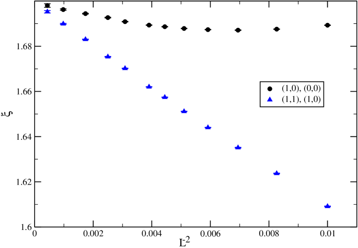
Figure 2: We plot $\xi_{2nd}$ as a function of $L^{-2}$, where $L$ is the linear extension in the transversal directions, for films of the thickness $L_{0}=6$. We have computed the second moment correlation length by using the pairs of wave vectors $(\,(0,0),(1,0)\,)$ (circles) and $(\,(1,0),(1,1)\,)$ (triangles).

Fitting the results obtained for $L=24$, $32$ and $48$ with the ansatz $\xi_{2nd}(L)=\xi_{2nd}+aL^{-2}$ we get $\xi_{2nd}=1.6988(6)$ and $1.6990(5)$ for the choices $(\,(0,0),(1,0)\,)$ and $(\,(1,0),(1,1)\,)$, respectively.

Next we have analyzed the energy per area, its first and second derivative with respect to $h_{1}$ and the magnetization $m_{1}$ at the surface. These quantities should converge with exponentially small corrections as $L\rightarrow\infty$. We have fitted these quantities with the ansatz $A(L)=A(\infty)+c_{A}\exp(-L/\xi_{film})$, where we have taken our result for the second moment correlation length $\xi_{2nd}=1.70$, which should not be much smaller than the exponential correlation length that is actually needed here. Fitting all data with $L\geq 16$ we find for the magnetization at the boundary $\chi^{2}$/DOF $=4.55/4$, $m_{1}(\infty)=0.1250175(6)$ and $c_{m_{1}}=-0.237(25)$. This means that for $L\approx 11\xi_{film}$ the deviation from the limit $L\rightarrow\infty$ has about the same size as the statistical error that we have reached here for $L_{0}=6$. Note that below, for larger thicknesses the number of measurements is more than a factor of ten smaller than for $L_{0}=6$. Analyzing the energy per area and its first and second derivative with respect to $h_{1}$ we find that for $L\approx 10\xi_{film}$ the deviation from the limit $L\rightarrow\infty$ has about the same size as the statistical error. Analyzing our results for the thickness $L_{0}=12$ we find consistently that for $m_{1}$ and the energy per area and its first and second derivative with respect to $h_{1}$, the deviation from the limit $L\rightarrow\infty$ has about the same size as the statistical error for $L\approx 10\xi_{film}$. As we shall see below, $\xi_{film}\approx 0.225(L_{0}+1.43)$. Therefore, for $L=4L_{0}$, which we have used below, the deviation from the limit $L\rightarrow\infty$ should be clearly smaller than the statistical error and can hence be ignored.

Next we have simulated films for a large number of thicknesses up to $L_{0}=64$ at $\beta=0.387721735$, using $L=4L_{0}$ throughout. For the thicknesses $L_{0}=6$, $7$, $8$, $9$, $10$, $11$, $12$, $13$, $14$, $15$, $16$, $18$, $20$, $22$, $24$ we performed $10^{8}$ update cycles throughout, and $7.6\times 10^{7}$, $10^{8}$, $8.7\times 10^{7}$, $6.5\times 10^{7}$, $4.3\times 10^{7}$, $2.6\times 10^{7}$, and $2.5\times 10^{7}$ update cycles for $L_{0}=28$, $32$, $36$, $40$, $48$, $56$, and $64$, respectively. These simulations took about 18 months of CPU time on a single core of a Quad-Core AMD Opteron(tm) Processor 2378 running at 2.4 GHz.

We have fitted the data of the magnetization $m_{1}$ at the surface with free boundary conditions with the ansatz

$$m_{1}=b\,(L_{0}+L_{s})^{2-y_{h_{1}}}$$ (48)

where $b$ and $y_{h_{1}}$ are the parameters of the fit and

$$m_{1}=b\,(L_{0}+L_{s})^{2-y_{h_{1}}}\times[1+c\,(L_{0}+L_{s})^{-2}]$$ (49)

where now $c$ is an additional parameter, to obtain some control on sub-leading corrections. We have taken into account all data obtained for the thicknesses $L_{0}\geq L_{0,min}$. Fitting our data with the ansatz (48) we get acceptable fits already for $L_{0,min}=10$: $b=1.6131(13)$, $L_{s}=1.4289(33)$, $y_{h_{1}}=0.72493(20)$, and $\chi^{2}/$DOF $=13.2/15$. Fitting with ansatz (49) we get for $L_{0,min}=6$ the results $b=1.6109(22)$, $L_{s}=1.4166(86)$, $y_{h_{1}}=0.72520(31)$, $c=-0.09(4)$, and $\chi^{2}/$DOF $=18.1/18$.

We arrive at the final estimates

$$b = 1.613(4)$$ (50)

$$L_{s} = 1.43(2)$$ (51)

$$y_{h_{1}} = 0.7249(6)$$ (52)

where the central result is taken from the fit with the ansatz (48) and $L_{0,min}=10$. The error bar is chosen such that also the result for the fit with sub-leading corrections (49) is covered. We have also estimated the error induced by the uncertainty of our estimate of the inverse bulk critical temperature $\beta_{c}$. To this end, we have first determined the derivative of $m_{1}$ with respect to $\beta$ for $L_{0}=8,9,12,13,16$ and $17$, where we performed simulations for many values of $\beta$. We have extrapolated these results to other values of $L_{0}$ assuming $\partial m_{1}/\partial\beta\propto(L_{0}+L_{s})^{2-y_{h_{1}}+y_{t}}$. Using this we have computed $m_{1}$ at $\beta=\beta_{c}+\mbox{error}=0.38772176$ and have redone the fits performed above. We find that the deviations of the results for $\beta=0.38772176$ from those for $\beta=0.387721735$ are much smaller than the errors quoted in eqs. (50,51,52).

Next we have analyzed the second moment correlation length obtained by using the pair $(\,(1,0),(1,1)\,)$ of wave vectors. Following the discussion above, finite $L$ effects might be still at the level of $1\%$ for our choice $L=4L_{0}$. Since this effect is essentially the same for all thicknesses, it mainly effects the parameter $c$ in the two equations below. First we have fitted our data with the ansatz

$$\xi_{2nd}=c\,(L_{0}+L_{s})$$ (53)

where $c$ and $L_{s}$ are the parameters of the fit. Using $L_{0,min}=8$ we obtain $c=0.22435(9)$, $L_{s}=1.487(6)$ and $\chi^{2}/$DOF $=19.2/18$. Fitting instead with the ansatz

$$\xi_{2nd}=c\,(L_{0}+L_{s})\times[1+b\,(L_{0}+L_{s})^{-2}]$$ (54)

we get for $L_{0,min}=6$ the results $c=0.22476(16)$, $L_{s}=1.422(20)$, $b=0.48(12)$ and $\chi^{2}/$DOF $=15.0/19$. We conclude that the estimate for $L_{s}$ obtained from the finite size scaling behavior of $\xi_{2nd}$ is consistent with but less precise than that obtained from the finite size scaling behavior of $m_{1}$.

Finally we have fitted the energy per area with the ansatz

$$E=L_{0}E_{ns}+E_{ns,s}+c\,(L_{0}+L_{s})^{-2+1/\nu}$$ (55)

where we have used $E_{ns}=0.602111(1)$ myamplitude and $\nu=0.63002(10)$ as input. Starting from our smallest thicknesses we get acceptable fits: For $L_{0,min}=6$ we obtain $c=-3.5916(7)$, $L_{s}=1.4136(21)$, $E_{ns,s}=3.0644(2)$ and $\chi^{2}/$DOF $=18.8/19$. As check we have also fitted with the ansatz

$$E=L_{0}E_{ns}+E_{ns,s}+c\,(L_{0}+L_{s})^{-2+1/\nu}\times[1+b\,(L_{0}+L_{s})^{-2}]$$ (56)

where we have included sub-leading corrections. For $L_{0,min}=6$ we get $c=-3.5930(15)$, $L_{s}=1.423(12)$, $E_{ns,s}=3.0646(2)$, $b=0.017(23)$ and $\chi^{2}/$DOF $=18.4/18$.

We have also redone the fits for shifted values of $E_{ns}$ and $\nu$. Since we have seen above in the case of $m_{1}$ that the uncertainty of $\beta_{c}$ is negligible, we have skipped this check here. Taking all these results into account we arrive at the final estimates

$$E_{ns,s} = 3.064(1)$$ (57)

$$L_{s} = 1.42(2)$$ (58)

$$c = 3.592(3)\;\;.$$ (59)

In particular we notice that the estimate of $L_{s}$ is fully consistent with that obtained above from the analysis of the magnetization $m_{1}$ at the boundary. In the following we shall use $L_{s}=1.43(2)$ as obtained from the analysis of the magnetization $m_{1}$ at the free boundary.

VI.2 The extrapolation length

First we have simulated lattices with $(h_{1},0)$ boundary conditions of the size $L_{0}=L=512$ at $\beta=0.387721735$ using $h_{1}=\beta_{c}$, $0.2$, $0.1$, $0.05$ and $0.02$. For this geometry one expects strong finite $L$ effects. However these should not alter the behavior in the neighborhood of the boundary that we study here. In all cases we have performed $2.6\times 10^{5}$ update cycles. In total these simulations took about 7 months of CPU time on a single core of a Quad-Core AMD Opteron(tm) Processor 2378 running at 2.4 GHz.

VI.2.1 Behavior of the magnetization at the free boundary

Following the discussion of section IV.1 we have determined the extrapolation length $l_{ex,ord}$ by fitting our data for the magnetization profile with the ansatz

$$m(z)=c\,(z+l_{ex,ord})^{(\beta_{1}-\beta)/\nu}$$ (60)

where $z$ gives the distance from the boundary as defined in section II.1, a few lines above eq. (16). To this end, we have computed the ratios

$$r(z)=m(z+1/2)/m(z-1/2)$$ (61)

to eliminate the constant in eq. (60). It turns out that cross-correlations of these ratios are relatively small. Therefore, for simplicity, we have fitted our data for these ratios taking only their statistical error into account, ignoring cross-correlations. The statistical errors of the fit-parameters were computed by using a Jackknife procedure on top of the whole analysis, providing us with correct statistical errors for the results.

First we have fitted our data with the ansatz

$$r(z)=\left(\frac{z+l_{ex,ord}+1/2}{z+l_{ex,ord}-1/2}\right)^{(\beta_{1}-\beta)/\nu}$$ (62)

where the free parameters of the fit are the extrapolation length $l_{ex,ord}$ and the exponent $(\beta_{1}-\beta)/\nu$. We have performed a large number of fits with various choices of the range $z_{min}\leq z\leq z_{max}$ of distances from the boundary that are taken into account, for all values of $h_{1}$ that we have simulated. The results for different $h_{1}$ are consistent among each other. In figure 3 we show our results for the exponent $(\beta_{1}-\beta)/\nu$ for the choice $z_{max}=3z_{min}$ as a function of $z_{min}$, where we have averaged over all values of $h_{1}$ that we have simulated. The error that we give is purely statistical. For comparison we plot the estimate of $(\beta_{1}-\beta)/\nu=2-y_{h_{1}}-(1+\eta)/2=0.7570(7)$ obtained by using our estimate of $y_{h_{1}}$, eq. (52), and $\eta=0.03627(10)$ mycritical .

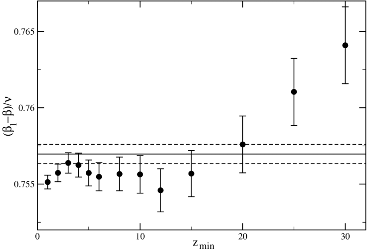
Figure 3: We plot the estimate of $(\beta_{1}-\beta)/\nu$ obtained by fitting with ansatz (62) as a function of $z_{min}$ (filled circles). In these fits distances $z_{min}\leq z\leq 3z_{min}$ from the boundary are taken into account. We have averaged the results over all values of $h_{1}$ that we have simulated. These results are compared with $(\beta_{1}-\beta)/\nu=2-y_{1}-(1+\eta)/2=0.7570(7)$ obtained by using $y_{h_{1}}=0.7249(6)$, see the previous section, and $\eta=0.03627(10)$ mycritical , where the central value is depicted by the solid line and the error-bars are indicated by the dashed lines.

We find that for $z_{min}=5$ up to $30$ the estimates obtained from the behavior of the magnetization profile in the neighborhood of the surface are consistent with but less precise than the one using the estimate of $y_{h_{1}}$ obtained in the previous section. Therefore, in order to determine our final result for the extrapolation length $l_{ex,ord}$, we have fixed $(\beta_{1}-\beta)/\nu=0.7570(7)$. Fitting the data for $r(z)$ averaged over all values of $h_{1}$ that we have simulated in the range $5\leq z\leq 30$ we arrive at

$$l_{ex,ord}=0.48(1)$$ (63)

where the error is dominated by the uncertainty of $(\beta_{1}-\beta)/\nu$.

VI.2.2 Normal extrapolation length as a function of $h_{1}$: part 1

Following the discussion of section IV.1 the magnetization in the neighborhood of the surface behaves as

$$m(z,h_{1})\propto(z+l_{ex,nor}(h_{1}))^{-\beta/\nu}$$ (64)

where $z$ gives the distance from the boundary. Also in the case of symmetry breaking boundary conditions, we have computed ratios (61) of the magnetization of neighboring slices. These behave as

$$r(z)=\left(\frac{z+l_{ex,nor}+1/2}{z+l_{ex,nor}-1/2}\right)^{-\beta/\nu}\;\;.$$ (65)

Here we have solved eq. (65) with respect to $l_{ex,nor}$ for a single value of $z$, where we have used $\beta/\nu=0.518135$. For $h_{1}=\beta_{c}$ we find for $z\approx 15$ only a small dependence of the result on $z$. We read off $l_{ex,nor}=0.96(2)$. In a similar way we have determined the extrapolation length for the other values of $h_{1}$. Our results are summarized in table 2.

Table 2: The extrapolation length $l_{ex,nor}$ is obtained for various values of $h_{1}$ by analyzing the behavior of the magnetization profile near the surface. For a discussion see the text.

$h_{1}$	$l_{ex,nor}$
$\beta_{c}$	0.96(2)
0.2	2.25(3)
0.1	5.56(4)
0.05	14.0(2)
0.02	$\approx 45$

In ref. mycritical we had determined $L_{s}=1.9(1)$ for $(+,+)$ and $(+,-)$ boundary conditions analyzing films of thicknesses up to $L_{0}=32$ at the critical point of the bulk system. Now we have added for $(+,+)$ boundary conditions simulations for the thicknesses $L_{0}=48$, $64$ and $96$. This allows us to improve the accuracy of our estimate. Now we find $L_{s}=1.90(5)$. This result is in perfect agreement with $L_{s}=2l_{ex,nor}(\beta_{c})=1.92(4)$ obtained here.

For $(0,+)$ boundary conditions we find $L_{s}=l_{ex,ord}+l_{ex,nor}(\beta_{c})=0.48(1)+0.96(2)=1.44(3)$, which is in perfect agreement with the result given in eq. (51) above.

VI.2.3 Normal extrapolation length as a function of $h_{1}$: part 2

Here we have simulated systems with $h_{1}h_{2}<0$, where $h_{2}=-\beta_{c}$, corresponding to fixed spins $s_{x}=-1$ at $x_{0}=L_{0}+1$, and various values of $h_{1}$. For such a choice of boundary conditions the magnetization profile takes positive values in the neighborhood of the first surface and negative ones in the neighborhood of the second surface. Therefore, in between the magnetization profile vanishes at $x_{0,zero}$, which depends on $h_{1}$ and $h_{2}$. The distance of this zero from the first boundary is given by $x_{0,zero}-1/2$ and from the second boundary by $L_{0}-x_{0,zero}+1/2$. Our basic assumption is that the zero of the magnetization indicates the physical middle of the system. Hence the distances of the zero from the effective positions of the first and the second boundary should be the same:

$$x_{0,zero}-1/2+l_{ex,nor}(h_{1})=L_{0}-x_{0,zero}+1/2+l_{ex,nor}(h_{2})$$ (66)

and hence

$$\Delta l_{ex,nor}(h_{1},h_{2})=l_{ex,nor}(h_{1})-l_{ex,nor}(h_{2})=L_{0}+1-2x_{0,zero}\;\;.$$ (67)

In order to define the zero of the magnetization we have linearly interpolated the magnetization profile. Throughout we simulate lattices with $L=4L_{0}$. First we have simulated at $h_{1}=0.2$, $0.1$ and $0.05$, using a large number of thicknesses $L_{0}$. Our results are summarized in table 3. Apparently, $\Delta l_{ex,nor}$ converges with an increasing thickness $L_{0}$. Numerically, corrections to the $L_{0}\rightarrow\infty$ limit are compatible with an exponential decay. However we can not strictly exclude power-like corrections. For $h_{1}=0.2$ our results for $L_{0}\geq 20$ are compatible within the statistical error. In the case of $h_{1}=0.1$ the results for $L_{0}=40$ and $48$ are compatible. The one for $L_{0}=64$ is larger by about twice the combined statistical error than that for $L_{0}=48$. For $h_{1}=0.05$ the results for $L_{0}=120$ and $160$ are compatible. It is natural to assume that the thickness $L_{0}$ needed to obtain $\Delta l_{ex,nor}$ with a given relative error is proportional to the extrapolation length $l_{ex,nor}(h_{1})$. Using $l_{ex,nor}(\beta_{c})=0.96(2)$ obtained in the section above, we conclude that for $L_{0}\gtrapprox 10l_{ex,nor}$ the deviation of $\Delta l_{ex,nor}$ from its $L_{0}\rightarrow\infty$ limit is less than the statistical error that we have reached here. Next we have simulated at $h_{1}=0.18$, $0.16$, $0.15$, $0.14$, $0.13$, $0.12$, $0.11$, $0.09$, $0.08$, $0.07$ and $0.06$ for a single thickness $L_{0}$ each. The thicknesses $L_{0}$ and the estimates for $\Delta l_{ex,nor}$ are given in table 3. Throughout $L_{0}>10l_{ex,nor}$ holds. For each of the simulations given in table 3 we performed about $10^{6}$ update cycles. In total these simulations took about 8 months of CPU time on a single core of a Quad-Core AMD Opteron(tm) Processor 2378 running at 2.4 GHz. Note that the results obtained here, are consistent with those of the previous section. Taking the numbers from table 2 we get $\Delta l_{ex,nor}=1.29(5)$, $4.60(6)$ and $13.04(22)$ for $h_{1}=0.2$, $0.1$ and $0.05$, which is perfectly consistent with the results of the present section, given in table 3.

Table 3: The difference of the extrapolation lengths $\Delta l_{ex,nor}(h_{1},h_{2})=l_{ex,nor}(h_{1})-l_{ex,nor}(h_{2})$, where $h_{2}=-\beta_{c}$ as a function of $h_{1}$. For a discussion see the text.

$h_{1}$	$L_{0}$	$\Delta l_{ex,nor}$
0.2	10	1.2642(21)
0.2	12	1.2748(25)
0.2	14	1.2829(27)
0.2	16	1.2889(32)
0.2	18	1.2852(35)
0.2	20	1.2955(38)
0.2	22	1.2989(42)
0.2	24	1.2938(44)
0.2	28	1.2932(54)
0.2	32	1.2941(62)
0.18	28	1.6182(47)
0.16	32	2.0434(61)
0.15	36	2.313(7)
0.14	42	2.606(9)
0.13	48	2.969(9)
0.12	54	3.401(10)
0.11	60	3.925(11)
0.1	16	4.187(4)
0.1	20	4.330(5)
0.1	24	4.407(6)
0.1	28	4.461(6)
0.1	32	4.488(7)
0.1	40	4.546(8)
0.1	48	4.543(10)
0.1	64	4.579(14)
0.09	80	5.399(13)
0.08	92	6.485(22)
0.07	110	7.917(25)
0.06	140	9.892(35)
0.05	24	10.194(7)
0.05	32	11.108(9)
0.05	40	11.682(11)
0.05	48	12.060(13)
0.05	56	12.279(16)
0.05	64	12.492(17)
0.05	80	12.668(21)
0.05	120	12.892(29)
0.05	160	12.899(42)

From eq. (30) follows that

$$\Delta l_{ex,nor}=l_{0}+l_{ex,nor,0}|h_{1}|^{-1/y_{h_{1}}}$$ (68)

where naively $l_{0}=l_{ex,nor}(\beta_{c})$. However, since $l_{ex,nor}$ depends on the precise definition of the thickness of the lattice, we keep the offset $l_{0}$ as a free parameter here.

It turns out that for the range of $h_{1}$ that we have simulated here, analytic corrections have to be taken into account. Therefore we have fitted our results for the difference of the extrapolation length with the ansatz

$$\Delta l_{ex,nor}=l_{0}+l_{ex,nor,0}|h_{1}+ah_{1}^{3}|^{-1/y_{h_{1}}}$$ (69)

where the amplitude $l_{ex,nor,0}$ , the offset $l_{0}$ and the correction amplitude $a$ are the parameters of the fit. Note that there should be no term $\propto h_{1}^{2}$ since $l_{ex,nor}(h_{1})=l_{ex,nor}(-h_{1})$. We set $y_{h_{1}}=0.7249(6)$ as obtained in section VI.1. In addition we have fitted with

$$\Delta l_{ex,nor}=l_{0}+l_{ex,nor,0}|h_{1}+ah_{1}^{3}+bh_{1}^{5}|^{-1/y_{h_{1}}}$$ (70)

to check for systematic errors due to the truncation of the Wegner expansion. Alternatively we have also fitted with

$$\Delta l_{ex,nor}=l_{0}+l_{ex,nor,0}|h_{1}|^{-1/y_{h_{1}}}\times(1+\tilde{a}h_{1}^{2})$$ (71)

and

$$\Delta l_{ex,nor}=l_{0}+l_{ex,nor,0}|h_{1}|^{-1/y_{h_{1}}}\times(1+\tilde{a}h_{1}^{2}+\tilde{b}h_{1}^{4})\;\;.$$ (72)

Fitting with the ansaetze (69,71) we get acceptable values of $\chi^{2}$/DOF starting from $h_{1,max}=0.2$, i.e. taking all data into account. Discarding data with large $h_{1}$ the result for $l_{ex,nor,0}$ is slightly decreasing and also $\chi^{2}$/DOF is further decreasing. E.g. fitting with ansatz (69) and taking $h_{1,max}=0.14$ we get $l_{ex,nor,0}=0.2133(9)$, $l_{0}=0.04(14)$, $a=6.9(2.2)$ and $\chi^{2}$/DOF $=1.72/7$. Taking into account the variation of the results over various ansaetze that we have used and the uncertainty of $y_{h_{1}}$ we arrive at

$$l_{ex,nor,0}=0.213(3)$$ (73)

which we shall use in the following.

VI.3 The thermodynamic Casimir force

We have computed the thermodynamic Casimir force per area and its first and second partial derivative with respect to $h_{1}$ for $(0,+)$ boundary conditions for the thicknesses $L_{0}=8.5$, $12.5$, and $16.5$. To this end we have simulated films of the thicknesses $L_{0}=8$, $9$, $12$, $13$, $16$ and $17$. For most of the simulations we have used $L=32$ for $L_{0}=8$ and $9$, $L=48$ for $L_{0}=12$ and $13$, and $L=64$ for $L_{0}=16$ and $17$. The correlation length of the film displays a single maximum at a temperature slightly below the critical temperature of the bulk system. The correlation length at the maximum is at most by one per mille larger than at the critical point of the bulk system. Therefore our choice of $L$ should ensure that finite $L$ effects of the energy per area and its first and second partial derivative with respect to $h_{1}$ can be safely ignored. At $\beta$-values that are much smaller or larger than $\beta_{c}$ we have used smaller values of $L$. Throughout we have checked that $L>10\xi_{film}$ is fulfilled with a clear safety margin. For $L_{0}=8$ and $9$ we have simulated at 85 values of the inverse temperature in the range $0.25\leq\beta\leq 0.5$, for $L_{0}=12$ and $13$ at 124 values in the rage $0.3\leq\beta\leq 0.42$, and for $L_{0}=16$ and $17$ at 112 values in the rage $0.34\leq\beta\leq 0.406$. The difference between neighboring $\beta$-values is adapted to the problem: It is the smallest close to $\beta_{c}$. We performed $10^{8}$ update cycles for $L_{0}=8$, $9$, $12$ and $13$ and $2\times 10^{8}$ update cycles for $L_{0}=16$ and $17$ for each value of $\beta$. In total these simulations took about 10 years of CPU time on a single core of a Quad-Core AMD Opteron(tm) Processor 2378 running at 2.4 GHz.

Using the estimates of the energy per area obtained from these simulations we have computed the thermodynamic Casimir force per area as discussed in section V. In figure 4 we have plotted $-L_{0,eff}^{3}\Delta f_{ex}$ as a function of $t(L_{0,eff}/\xi_{0})^{1/\nu}$, where we have used $L_{0,eff}=L_{0}+L_{s}$ with $L_{s}=1.43$ obtained above in section VI.1. We do not show statistical errors in figure 4, since they are comparable with the thickness of the lines. The curves for $L_{0}=8.5$, $12.5$ and $16.5$ fall quite nicely on top of each other. Only for $x\lessapprox-7$, in the low temperature phase, we see a small discrepancy between the result for $L_{0}=8.5$, $12.5$ and $16.5$, which might be attributed to analytic corrections. We conclude that we have obtained a good approximation of the finite size scaling function $\theta_{(0,+)}$.

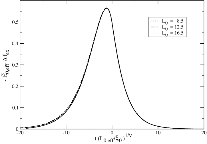
Figure 4: We plot $-L_{0,eff}^{3}\Delta f_{ex}$ as a function of $t(L_{0,eff}/\xi_{0})^{1/\nu}$ for $(0,+)$ boundary conditions for the thicknesses $L_{0}=8.5$, $12.5$ and $16.5$. To this end, we have used $L_{0,eff}=L_{0}+L_{s}$ with $L_{s}=1.43$, $\xi_{0}=0.2282$ and $\nu=0.63002$.

Throughout $\theta_{(0,+)}$ is positive, which means that the thermodynamic Casimir force is repulsive. The scaling function $\theta_{(0,+)}$ has a single maximum. We have determined the position of this maximum from the zero of $\Delta E$. We find $\beta_{max}=0.39069(2)$, $0.389443(10)$, and $0.388874(6)$ for $L_{0}=8.5$, $12.5$, and $16.5$, respectively. It follows $x_{t,max}=t_{max}(L_{0,eff}/\xi_{0})^{1/\nu}=$ $-1.184(13)$, $-1.175(11)$, and $-1.174(10)$ for $L_{0}=8.5$, $12.5$, and $16.5$, respectively. The error bar includes the uncertainties of $\beta_{max}$, $L_{s}$ and $\nu$. Note that the results obtained from the three different thicknesses are consistent. Next we have determined the value of the scaling function at the maximum. We get $-L_{0,eff}^{3}\Delta f_{ex}(x_{t,max})$ = $0.567(4)$, $0.566(3)$, and $0.564(3)$ for $L_{0}=8.5$, $12.5$ and $16.5$, respectively. The error is dominated by the uncertainty of $L_{s}$. The results obtained from the three different thicknesses are consistent. As the final result we take the one obtained from $L_{0}=16.5$:

$$x_{t,max}=-1.174(10)\;\;,\;\;\;\theta_{(0,+),max}=0.564(3)\;\;.$$ (74)

At the critical point of the bulk system, the finite size scaling function assumes the value

$$\theta_{(0,+)}(0)=0.497(3)$$ (75)

where the error is dominated by the uncertainty of $L_{s}$. This results can be compared with $\theta_{(0,+)}(0)=0.33$, $0.416$ and $0.375(14)$ obtained by using the $\epsilon$-expansion, and Monte Carlo simulations of the Ising model Krech97 . Similar to the case of $(+,+)$ and $(+,-)$ boundary conditions myCasimir , we see a large deviations of the results of Krech from ours.

In figure 5 we compare the finite size scaling function of the thermodynamic Casimir force per area for $(0,+)$ boundary conditions with those of $(+,+)$ and $(+,-)$ boundary conditions that we have obtained in myCasimir .

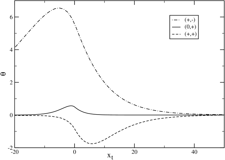
Figure 5: We plot our result for the finite size scaling function $\theta_{(0,+)}$ along with those for $\theta_{(+,+)}$ and $\theta_{(+,-)}$ obtained in ref. myCasimir .

In the high temperature phase and around the bulk critical point, the absolute value of $\theta_{(0,+)}$ is smaller than that of $\theta_{(+,+)}$, while in the low temperature phase for $x_{t}\lessapprox-1.1$ it becomes larger. The value of $\theta_{(0,+)}$ is much smaller than that of $\theta_{(+,-)}$ throughout.

As discussed in ref. Krech97 , see in particular eq. (3.6) and the Appendix A of ref. Krech97 , in the mean-field approximation there is a simple relation between the scaling functions $\theta_{(+,-)}$ and $\theta_{(+,0)}$. For $(+,-)$ boundary conditions, the magnetization vanishes in the middle of the film. Hence, ignoring fluctuations, a film of the thickness $2L_{0}$ with $(+,-)$ boundary conditions is composed of two films of the thickness $L_{0}$, where one has $(+,0)$ and the other $(0,-)$ boundary conditions. Furthermore $(0,+)$, $(+,0)$ and $(0,-)$ boundary conditions are equivalent. Therefore

$$\theta_{MF,(0,+)}(x_{t})=2^{-d}\theta_{MF,(+,-)}(2^{1/\nu}x_{t})\;\;.$$ (76)

For less than four dimensions one expects deviations from this relation. Indeed for the Ising bulk universality class the ratio of Casimir amplitudes

$$\frac{\Delta_{(+,-)}}{\Delta_{(0,+)}}=16(1-0.481\epsilon+...)$$ (77)

obtained by using the $\epsilon$-expansion Krech97 clearly differs from $2^{4-\epsilon}=16(1-0.6931...\epsilon+...)$ obtained from eq. (76). Note that the Casimir amplitude is given by $2\Delta_{(b_{1},b_{2})}=\theta_{(b_{1},b_{2})}(0)$. For two dimensions one obtains from conformal field theory Cardy86

$$\frac{\Delta_{(+,-)}}{\Delta_{(+,0)}}=\frac{23}{2}$$ (78)

which is almost 3 times as large as the factor $4$ predicted by eq. (76).

Taking our numerical data, we find for $x_{t}>0$, this means in the high temperature phase, $\theta_{(+,0)}(x_{t})\approx 0.7\times 2^{-3}\theta_{(+,-)}(2^{1/0.63002}x_{t})$, while in the low temperature phase, one gets $\theta_{(+,0)}(x_{t})\approx 2^{-3}\theta_{(+,-)}(2^{1/0.63002}x_{t})-0.3$ in the range $-10<x_{t}<-3$. This means that eq. (76) does not provide a quantitatively accurate relation between the scaling functions $\theta_{(+,0)}(x_{t})$ and $\theta_{(+,-)}(x_{t})$ in the three dimensional case.

The most striking observation is that in the high temperature phase $\theta_{(0,+)}$ decays, with increasing $x_{t}$, much faster to zero than $\theta_{(+,+)}$ and $\theta_{(+,-)}$ do. This behavior can be explained by using the transfer matrix formalism. For a discussion of the transfer matrix formalism applied to the problem of the thermodynamic Casimir effect see section IV of myCasimir . In terms of eigenvalues $\lambda_{\alpha}$ and eigenvectors $|\alpha\rangle$ of the transfer matrix the thermodynamic Casimir force per area can be written as

$$\frac{1}{k_{B}T}F_{Casimir}=-\frac{1}{L^{2}}\;\frac{\sum_{\alpha}m_{\alpha}\exp(-m_{\alpha}l)\;\langle b_{1}|\alpha\rangle\langle b_{2}|\alpha\rangle}{\sum_{\alpha}\exp(-m_{\alpha}l)\;\langle b_{1}|\alpha\rangle\langle b_{2}|\alpha\rangle}$$ (79)

where $1/\xi_{\alpha}=m_{\alpha}=-\ln(\lambda_{\alpha}/\lambda_{0})$. Note that here $m$ is a mass and should not be confused with the magnetization. We assume that the eigenvalues are ordered such that $\lambda_{\alpha}\geq\lambda_{\beta}$ for $\alpha<\beta$, where $\alpha$, $\beta$ are positive integers or zero. The states $|b_{1}\rangle$ and $|b_{2}\rangle$ are defined by the boundary conditions that are applied and $l=L_{0}+1$. For $x_{t}\gg 0$ the right side of eq. (79) is dominated by the contribution from the state $|1\rangle$ and therefore

$$\tilde{\theta}_{(b_{1},b_{2})}(ml)\approx-m^{3}l^{3}\exp(-ml)C(b_{1})C(b_{2})$$ (80)

where we have identified $1/\xi=m=m_{1}$ and have defined

$$C(b)=\frac{1}{mL}\frac{\langle b|1\rangle}{\langle b|0\rangle}\;\;.$$ (81)

The state $|0\rangle$ is symmetric under the global transformation $s_{x}\rightarrow-s_{x}$ for all $x$ in a slice. Instead, $|1\rangle$ is anti-symmetric and therefore $C=C(+)=-C(-)$. It follows

$$\tilde{\theta}_{(+,+)}(ml)=-\tilde{\theta}_{(+,-)}(ml)=-C^{2}\;m^{3}l^{3}\exp(-ml)$$ (82)

for sufficiently large values of $ml$. Since $x_{t}=t[l/\xi_{0}]^{1/\nu}\simeq(ml)^{1/\nu}$ it follows

$$\theta_{(+,+)}(x_{t})=-\theta_{(+,-)}(x_{t})=-C^{2}x_{t}^{3\nu}\exp(-x_{t}^{\nu})$$ (83)

for sufficiently large values of $x_{t}$. In the case of free boundary conditions the boundary state $|0\rangle$ is symmetric under the global transformation $s_{x}\rightarrow-s_{x}$. Therefore $\langle b|1\rangle$ vanishes and therefore

$$C(0)=0\;\;.$$ (84)

Next we have studied the first derivative of the scaling function with respect to $h_{1}$. In figure 6 we have plotted $-L_{0,eff}^{3}(L_{0,eff}/l_{ex,nor,0})^{-y_{h_{1}}}\frac{\partial\Delta f_{ex}}{\partial h_{1}}$ as a function of $t(L_{0,eff}/\xi_{0})^{1/\nu}$. We do not give error bars, since the statistical error is of similar size as the thickness of the lines. We find that the data for $L_{0}=8.5$, $12.5$ and $16.5$ fall quite nicely on top of each other. The small discrepancies that are visible for large absolute values of $x_{t}$ might be attributed to analytic corrections. We conclude that our numerical results provide a good approximation of the finite size scaling function $\theta^{\prime}(x_{t})\equiv\left.\frac{\partial\Theta(x_{t},x_{h_{1}})}{\partial h_{1}}\right|_{h_{1}=0}$. We read off from figure 6 that $\theta^{\prime}$ is negative throughout and has a single minimum.

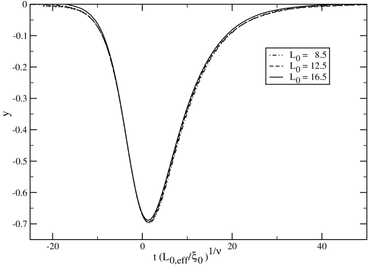
Figure 6: We plot $y=-L_{0,eff}^{3}(L_{0,eff}/l_{ex,nor,0})^{-y_{h_{1}}}\frac{\partial\Delta f_{ex}}{\partial h_{1}}$ as a function of $t(L_{0,eff}/\xi_{0})^{1/\nu}$ for $(0,+)$ boundary conditions for the thicknesses $L_{0}=8.5$, $12.5$ and $16.5$. To this end, we have used $L_{0,eff}=L_{0}+L_{s}$ with $L_{s}=1.43$, $\xi_{0}=0.2282$ and $\nu=0.63002$.

We have determined the location of this minimum by searching for the zero of $\frac{\partial\Delta E}{\partial h_{1}}$. We find $\beta_{min}=0.38403(3)$, $0.38577(2)$ and $0.38645(2)$ for $L_{0}=8.5$, $12.5$ and $16.5$, respectively. This corresponds to $x_{t,min}=1.473(18)$, $1.333(18)$, and $1.296(24)$. Here we have taken into account the errors of $\beta_{min}$, $L_{s}$ and $\nu$. In particular for $L_{0}=16.5$ the error of $\beta_{min}$ clearly dominates. The results for $L_{0}=12.5$ and $16.5$ are consistent. As value of the derivative of the scaling function we obtain $-0.697(13)$, $-0.696(14)$ and $-0.688(13)$ for $L_{0}=$ $8.5$, $12.5$ and $16.5$, respectively. Note that in all cases about half of the error is due to the uncertainty in $l_{ex,nor,0}=0.213(3)$. The results for the different lattice sizes are consistent within the quoted errors. We conclude

$$x_{t,min}=1.30(5)\;\;\;,\;\;\;\theta^{\prime}_{min}=-0.69(2)\;\;.$$ (85)

Assuming that $C(h_{1})$ is an analytic function and the finite size scaling behavior (35) of the thermodynamic Casimir force per area we arrive at

$$\theta^{\prime}(x_{t})=Bx_{t}^{3\nu-\Delta_{1}}\exp(-x_{t}^{\nu})$$ (86)

for $x_{t}\gg 0$. Matching our numerical data for $L_{0}=16.5$ at $x_{t}\approx 10$ with eq. (86) we arrive at $B=-0.85(5)$, where the error is estimated by comparing with the result obtained from $L_{0}=12.5$.

Next we have studied the second derivative of the scaling function with respect to $h_{1}$. To this end, in figure 7 we have plotted $-L_{0,eff}^{3}(L_{0,eff}/l_{ex,nor,0})^{-2y_{h_{1}}}\frac{\partial^{2}\Delta f_{ex}}{\partial h_{1}^{2}}$ as a function of $t(L_{0,eff}/\xi_{0})^{1/\nu}$. For $L_{0}=16.5$ we have plotted the statistical error, which we have not done for $L_{0}=8.5$, $12.5$ to keep the figure readable. Within our statistical accuracy, the curves for the three different thicknesses fall on top of each other. It seems that $\theta^{\prime\prime}$ is positive for all values of the scaling function. Likely the negative values found for large $|x_{t}|$ and $L_{0}=16.5$ are just an artifact due to statistical fluctuations. The function displays a single maximum that is located at

$$x_{t,min}=-1.9(2)\;\;\;,\;\;\;\theta^{\prime\prime}_{min}=-0.39(2)\;\;.$$ (87)

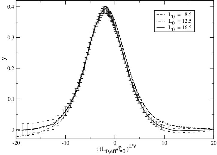
Figure 7: We plot $y=-L_{0,eff}^{3}(L_{0,eff}/l_{ex,nor,0})^{-2y_{h_{1}}}\frac{\partial^{2}\Delta f_{ex}}{\partial h_{1}^{2}}$ as a function of $t(L_{0,eff}/\xi_{0})^{1/\nu}$ for $(0,+)$ boundary conditions for the thicknesses $L_{0}=8.5$, $12.5$ and $16.5$. To this end, we have used $L_{0,eff}=L_{0}+L_{s}$ with $L_{s}=1.43$, $\xi_{0}=0.2282$ and $\nu=0.63002$.

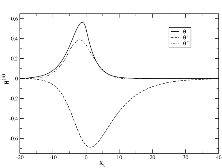
Figure 8: We plot $\theta_{(0,+)}$, $\theta_{(0,+)}^{\prime}$ and $\theta_{(0,+)}^{\prime\prime}$ as a function of $x_{t}$.

In figure 8 we have plotted $\theta_{(0,+)}$, $\theta_{(0,+)}^{\prime}$ and $\theta_{(0,+)}^{\prime\prime}$. To this end we have used the results obtained for $L_{0}=16.5$. We find that the shape of $\theta_{(0,+)}^{\prime\prime}$ is quite similar to that of $\theta_{(0,+)}$. In particular, for $x_{t}\rightarrow\infty$, both $\theta_{(0,+)}$ and $\theta_{(0,+)}^{\prime\prime}$ approach zero much faster than $\theta_{(0,+)}^{\prime}$. Therefore already for an infinitesimally small positive value of $x_{h_{1}}$, the crossover scaling function $\Theta(x_{t},x_{h_{1}})$, taken as a function of $x_{t}$, has a minimum in the high temperature phase.

In order to check the range of applicability of the Taylor-expansion, and to study the crossover beyond the Taylor-expansion, we have simulated films with $(h_{1},+)$ boundary conditions and the thicknesses $L_{0}=8$ and $9$ at the values $h_{1}=0.03$, $0.06$, $0.1$ and $0.2$ of the external field at the boundary. Our results along with that for $(+,+)$ corresponding to $h_{1}=\beta$ obtained in myCasimir are plotted in figure 9. For $h_{1}=0.03$ there is a minimum of the thermodynamic Casimir force per area in the high temperature phase. Its absolute value is about one third of the value of the maximum in the low temperature phase. The thermodynamic Casimir force changes sign at $\beta\approx 0.384$, which is slightly smaller than $\beta_{c}$. Going to larger values of $h_{1}$ the position of the minimum changes only little and the absolute value of the minimum increases. On the other hand, the value of the maximum is decreasing with increasing $h_{1}$. For $h_{1}=0.2$, the maximum has vanished.

The authors of MoMaDi10 show in figure 9 of their paper Monte Carlo data obtained by O. Vasilyev Va for the three-dimensional Ising model and the film thickness $L_{0}=10$. There is nice qualitative agreement with our results given in figure 9.

We have compared the results for the thermodynamic Casimir force per area obtained by simulating at $h_{1}=0.03$, $0.06$, $0.1$ and $0.2$ for $L_{0}=8.5$ with those obtained by the Taylor-expansion around $h_{1}=0$ up to second order in $h_{1}$. We find that for $h_{1}=0.03$ the results almost agree within the statistical error. Still for $h_{1}=0.06$ the Taylor-expansion to second order resembles the true result quite well. The largest discrepancy is found for the value of the maximum of the thermodynamic Casimir force per area. It is overestimated by about a factor of $1.24$. As one might expect, the result of the Taylor-expansion becomes increasingly worse with increasing $h_{1}$. In particular it does not reproduce that for large values of $h_{1}$ the maximum of the thermodynamic Casimir force per area disappears.

Figure 9: We plot $-\Delta f_{ex}$ for $(h_{1},+)$ boundary conditions as a function of the reduced temperature $\beta_{c}-\beta$. The thickness of the film is $L_{0}=8.5$ throughout.

Given our results for various thicknesses $L_{0}$ at $h_{1}=0$, we conclude that the results for $L_{0}=8.5$ provide already a quite good approximation of the scaling limit. In particular we are confident that the qualitative features of the crossover discussed here still hold in the scaling limit. In particular we conclude that for $x_{h_{1}}\lessapprox 0.03[(8.5+1.43)/0.213]^{0.7249}\approx 0.5$ the scaling function $\Theta(x_{t},x_{h_{1}})$ is still well described by the Taylor-expansion around $x_{h_{1}}=0$ to second order.

From figure 9 we can read off that the thermodynamic Casimir force can also change sign as a function of the thickness $L_{0}$ for fixed values of $h_{1}$ and the temperature. In general both $x_{t}=t[L_{0}/\xi_{0}]^{y_{t}}$ and $x_{h_{1}}=h_{1}[L_{0}/l_{ex,nor,0}]^{y_{h_{1}}}$ depend on the thickness $L_{0}$. Therefore, for simplicity let us consider the bulk critical temperature, where $x_{t}=0$ for any thickness of the film. For small $L_{0}$ the scaling variable $x_{h_{1}}$ is small and therefore the thermodynamic Casimir force is close to the case $x_{h_{1}}=0$ and is therefore repulsive. As $L_{0}$ increases, $x_{h_{1}}$ increases and therefore $\Theta(0,x_{h_{1}})$ decreases. We read off from figure 9 that $\Theta(0,x_{h_{1}})\approx 0$ for $x_{h_{1}}\approx 1$. With further increasing $L_{0}$, the thermodynamic Casimir force becomes attractive.

VI.3.1 Approach to the $h_{1}\rightarrow\infty$ limit

For sufficiently large values of $x_{h_{1}}=h_{1}(L_{0}/l_{ex,nor,0})^{y_{h_{1}}}$ we expect that corrections to the $x_{h_{1}}\rightarrow\infty$ limit can be described by replacing $L_{0}$ by $L_{0,eff}=L_{0}+L_{s}$, where

$$L_{s}=l_{ex,nor}(h_{1})+l_{ex,nor}(h_{2})\;\;.$$ (88)

In figure 10 we have plotted our results for $h_{1}=0.2$ and $L_{0}=8.5$ and $L_{0}=16.5$. First we use $L_{s}=1.9$ that we had obtained in ref. myCasimir for $(+,+)$ boundary conditions and second $L_{s}=1.9+1.294$, where we have added $\Delta l_{ex,nor}(0.2,\beta_{c})$ obtained in section VI.2 above. For comparison we give the result obtained for $L_{0}=16.5$ and $(+,+)$ boundary conditions, using $L_{s}=1.9$. In the case of $L_{0}=8.5$ the matching with the $(+,+)$ result is somewhat improved by using $L_{s}=1.9+1.294$ instead of $L_{s}=1.9$. While the value of the minimum is clearly improved, the matching of the curve with that for $(+,+)$ boundary conditions deep in the high temperature phase is not. In contrast, for $L_{0}=16.5$, using $L_{s}=1.9+1.294$ instead of $L_{s}=1.9$ clearly improves the matching of the curve for $h_{1}=0.2$ with that for $h_{1}=\beta$ in the whole range of $x_{t}$ that is considered.

We conclude that for $L_{0}\gtrapprox 10\Delta l_{ex,nor}(h_{1},\beta_{c})$ using $L_{s}=1.9+\Delta l_{ex,nor}(h_{1},\beta_{c})$ clearly improves the matching with the $(+,+)$ scaling function. It would be desirable to check this by simulations for smaller values of $h_{1}$. However this would be quite expensive, since already for $h_{1}=0.15$ we would need to simulate a thickness $L_{0}\approx 30$.

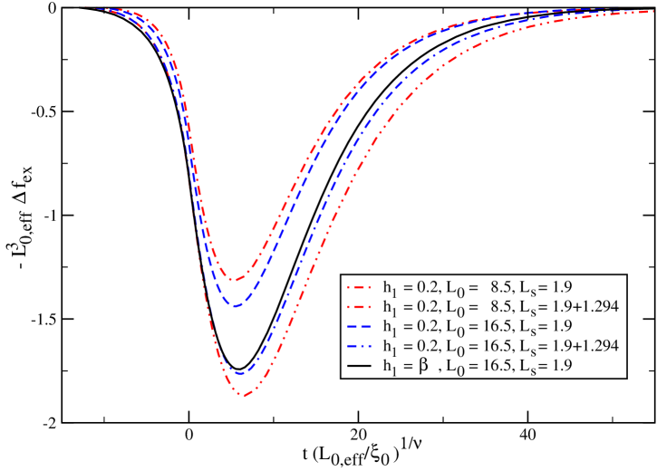
Figure 10: We plot $L_{0,eff}^{3}\Delta f_{ex}$ as a function of $t(L_{0,eff}/\xi_{0})^{1/\nu}$ for $h_{1}=0.2$ and $L_{0}=8.5$ and $16.5$ using $L_{s}=1.9$ or $L_{s}=1.9+1.294$. For comparison we give the corresponding curve for $L_{0}=16.5$ and $(+,+)$ boundary conditions using $L_{s}=1.9$. For a discussion see the text.

VII Summary and conclusions

We have studied the crossover behaviors of a surface of a system in three-dimensional Ising universality class from the ordinary to the normal or extraordinary surface universality class. To this end, we have simulated the improved Blume-Capel model on the simple cubic lattice. In particular we have studied films with various boundary conditions applied. Improved means that corrections to finite size scaling $\propto L_{0}^{-\omega}$ have a vanishing amplitude, where $L_{0}$ is the thickness of the film and $\omega=0.832(6)$ mycritical is the exponent of leading corrections. This property is very useful in the study of films, since corrections $\propto L_{0}^{-1}$ due to the surfaces are expected DiDiEi83 and fitting data it is difficult to disentangle corrections with similar exponents such as $\omega$ and one. Mostly we have simulated films with $(0,+)$ boundary conditions. This means that at one surface we apply free boundary conditions, while at the other surface the spins are fixed to $+1$. Studying the magnetization of the slice at the surface with free boundary conditions, at the bulk critical point, of films of a thickness up to $L_{0}=64$ we arrive at the estimate $y_{h_{1}}=0.7249(6)$ for the renormalization group exponent of the external field at the surface for the ordinary surface universality class. This estimate is at least by a factor of 5 more accurate than those previously given in the literature. The authors of DeBlNi05 quote an error that is only 2.5 times larger than ours, however the deviation between our and their estimate is about 6 times larger than the combined errors. For details see table 1. We have studied the magnetization profile in the neighborhood of the surfaces for both the ordinary as well as the normal surface universality class. The data are consistent with the theoretically predicted power law behavior. This study also allowed us to determine the extrapolation length $l_{ex}$ for free boundary conditions as well as symmetry breaking boundary conditions for various values of the external field $h_{1}$ at the surface. Corrections to scaling $\propto L_{0}^{-1}$, which are due to the surfaces of the film can be expressed by an effective thickness $L_{0,eff}=L_{0}+L_{s}$, where $L_{s}$ depends on the details of the model. Our numerical results confirm the hypothesis that $L_{s}=l_{ex,1}+l_{ex,2}$, where $l_{ex,1}$ and $l_{ex,2}$ are the extrapolation lengths at the two surfaces of the film.

Next we have studied the thermodynamic Casimir force in the neighborhood of the bulk critical point in the range of temperatures where it does not vanish at the level of our accuracy. First we have simulated films with $(0,+)$ boundary conditions and the thicknesses $L_{0}=8.5$, $12.5$ and $16.5$. Taking into account corrections by replacing $L_{0}$ by $L_{0,eff}$, the behavior of the thermodynamic Casimir force and its first and second derivative with respect to $h_{1}$ follows quite nicely the predictions of finite size scaling. Hence our data allow us to compute good estimates of the finite size scaling functions $\theta_{(0,+)}$, $\theta_{(0,+)}^{\prime}$, and $\theta_{(0,+)}^{\prime\prime}$. Next we have computed the thermodynamic Casimir force per area for the thickness $L_{0}=8.5$ at the finite values $h_{1}=0.03$, $0.06$, $0.1$ and $0.2$ of the external field at the boundary. We find that the Taylor-expansion of the thermodynamic Casimir force up to the second order in $h_{1}$ around $h_{1}=0$ still describes the full function well at $h_{1}=0.03$ which corresponds to the value $x_{h_{1}}=h_{1}[L_{0}/l_{0,ex,nor}]^{y_{h_{1}}}\approx 0.5$ of the scaling variable of the external field at the boundary. Finally, we have studied the approach of the thermodynamic Casimir force to the limit $h_{1}\rightarrow\infty$. We find that by using $L_{0,eff}=L_{0}+L_{s}(h_{1})$, the corrections to this limit are well described for $L_{0}\gtrapprox 10[L_{s}(h_{1})-L_{s}(\beta_{c})]$.

Based on exact results for stripes of the two-dimensional Ising model AbMa09 , mean-field calculations MoMaDi10 and preliminary Monte Carlo results for the Ising model Va on the simple cubic lattice one expects that for certain combinations of the external fields $h_{1}$, $h_{2}$ and the thickness of the lattice $L_{0}$, the thermodynamic Casimir force changes sign as a function of the temperature. Also for certain choices of the external fields $h_{1}$, $h_{2}$ and the temperature, the thermodynamic Casimir force changes sign as a function of the thickness of the film. Here we confirm these qualitative findings.

VIII Acknowledgements

This work was supported by the DFG under the grant No HA 3150/2-1.

References

- (1) M. E. Fisher and P.-G. de Gennes, CR Seances Acad. Sci. Ser. B 287, 207 (1978).
- (2) H. B. G. Casimir, Proc. K. Ned. Akad. Wet. 51, 793 (1948).
- (3) A. Gambassi, J. Phys. Conf. Series 161, 012037 (2009) [arXiv:0812.0935].
- (4) M. N. Barber, “Finite-size Scaling” in Phase Transitions and Critical Phenomena, Vol. 8, eds. C. Domb and J. L. Lebowitz, (Academic Press, London, 1983)
- (5) Krech M, The Casimir Effect in Critical Systems (World Scientific, Singapore, 1994)
- (6) K. G. Wilson and J. Kogut, Phys. Rep. C 12, 75 (1974).
- (7) M. E. Fisher, Rev. Mod. Phys. 46, 597 (1974).
- (8) M. E. Fisher, Rev. Mod. Phys. 70, 653 (1998).
- (9) A. Pelissetto and E. Vicari, Phys. Rept. 368, 549 (2002) [arXiv:cond-mat/0012164]
- (10) K. Binder, “Critical Behaviour at Surfaces” in Phase Transitions and Critical Phenomena, Vol. 8, eds. C. Domb and J. L. Lebowitz, (Academic Press, London, 1983)
- (11) H. W. Diehl, Field-theoretical Approach to Critical Behaviour at Surfaces in Phase Transitions and Critical Phenomena, edited by C. Domb and J.L. Lebowitz, Vol. 10 (Academic Press, London, 1986) p. 76.
- (12) H. W. Diehl, Int. J. Mod. Phys. B 11, 3503 (1997) [arXiv:cond-mat/9610143]
- (13) Felix M. Schmidt and H. W. Diehl, Phys. Rev. Lett. 101, 100601 (2008) [arXiv:0806.2799]
- (14) D. B. Abraham and A. Maciołek, Phys. Rev. Lett. 105, 055701 (2010) [arXiv:0912.0104]
- (15) T. F. Mohry, A. Maciołek, and S. Dietrich, Phys. Rev. E 81, 061117 (2010) [arXiv:1004.0112]
- (16) O. Vasilyev, private communication to the authors of MoMaDi10 . Further preliminary results were presented as poster at the Workshop ”Fluctuation-Induced Forces in Condensed Matter” Dresden, 11 - 15 October 2010. http://www.mpipks-dresden.mpg.de/fifcm10/
- (17) P. Ball, Nature 447, 772 (2007).
- (18) U. Nellen, L. Helden, and C. Bechinger Europhys. Lett. 88, 26001 (2009) [arXiv:0910.2373]
- (19) M. Tröndle, S. Kondrat, A. Gambassi, L. Harnau, and S. Dietrich, Europhys. Lett. 88, 40004 (2009) [arXiv:0903.2113]
- (20) M. Tröndle, S. Kondrat, A. Gambassi, L. Harnau, and S. Dietrich J. Chem. Phys. 133, 074702 (2010) [arXiv:1005.1182]
- (21) A. Gambassi and S. Dietrich, Soft Matter 7, 1247 (2011) [arXiv:1011.1831]
- (22) M. Tröndle, O. Zvyagolskaya, A. Gambassi, D. Vogt, L. Harnau, C. Bechinger, and S. Dietrich, preprint [arXiv:1012.0181]
- (23) B. V. Derjaguin, Kolloid Z. 69, 155 (1934)
- (24) A. Hanke, F. Schlesener, E. Eisenriegler, and S. Dietrich, Phys. Rev. Lett. 81, 1885 (1998)
- (25) F. Schlesener, A. Hanke, and S. Dietrich, J. Stat. Phys. 110, 981 (2003)
- (26) C. Hertlein, L. Helden, A. Gambassi, S. Dietrich, and C. Bechinger, Nature 451, 172 (2008)
- (27) A. Gambassi, A. Maciołek, C. Hertlein, U. Nellen, L. Helden, C. Bechinger, and S. Dietrich, Phys. Rev. E 80, 061143 (2009) [arXiv:0908.1795]
- (28) O. Vasilyev, A. Gambassi, A. Maciołek, and S. Dietrich, Europhys. Lett. 80, 60009 (2007) [arXiv:0708.2902]
- (29) O. Vasilyev, A. Gambassi, A. Maciołek, and S. Dietrich, Phys. Rev. E 79, 041142 (2009) [arXiv:0812.0750]
- (30) M. Hasenbusch, Phys. Rev. B 82, 104425 (2010) [arXiv:1005.4749]
- (31) A. Hucht, Phys. Rev. Lett. 99, 185301 (2007) [arXiv:0706.3458]
- (32) M. Krech and D. P. Landau, Phys. Rev. E 53, 4414 (1996)
- (33) M. Hasenbusch, Phys. Rev. E 80, 061120 (2009) [arXiv:0908.3582]
- (34) D. Dantchev and M. Krech, Phys. Rev. E 69, 046119 (2004) [arXiv:cond-mat/0402238]
- (35) Y. Deng and H. W. J. Blöte, Phys. Rev. E 70, 046111 (2004).
- (36) M. Hasenbusch, Phys. Rev. B 82, 174433 (2010) [arXiv:1004.4486]
- (37) M. Hasenbusch, Phys. Rev. B 82, 174434 (2010) [arXiv:1004.4983]
- (38) C. J. Silva, A. A. Caparica, and J. A. Plascak, Phys. Rev. E 73, 036702 (2006).
- (39) T. W. Burkhardt and H. W. Diehl, Phys. Rev. B 50, 3894 (1994).
- (40) T. W. Burkhardt and E. Eisenriegler, Phys. Rev. B 16, 3213 (1977); Phys. Rev. B 17, 318 (1978).
- (41) S. G. Whittington, G. M. Torrie and A. J. Guttmann, J. Phys. A: Math. Gen. 19, 2449 (1979).
- (42) H. W. Diehl and S. Dietrich, Z. Phys. B 42, 65 (1981).
- (43) H. W. Diehl and M. Shpot, Nucl. Phys. B 528, 595 (1998).
- (44) K. Binder and D. P. Landau, Phys. Rev. Lett. 52, 318 (1984).
- (45) M. Kikuchi and Y. Okabe, Prog. Theor. Phys. 73, 32 (1985).
- (46) D. P. Landau and K. Binder, Phys. Rev. B 41, 4633 (1990).
- (47) M. P. Nightingale and H. W. J. Blöte, Phys. Rev. B 48, 13678 (1993).
- (48) C. Ruge and F. Wagner, Phys. Rev. B 52, 4209 (1995).
- (49) M. Pleimling and W. Selke, Eur. Phys. J. B 1, 385 (1998) [arXiv:cond-mat/9710097]
- (50) Y. Deng and H. W. J. Blöte, Phys. Rev. E 67, 066116 (2003).
- (51) Y. Deng, H. W. J. Blöte, and M. P. Nightingale, Phys. Rev. E 72, 016128 (2005) [arXiv:cond-mat/0504173].
- (52) S. Z. Lin and B. Zheng, Phys. Rev. E 78, 011127 (2008).
- (53) M. Smock, H. W. Diehl, and D. P. Landau, Ber. Bunsenges. Phys. Chem. 98, 486 (1994) [arXiv:cond-mat/9402068].
- (54) H. W. Diehl, S. Dietrich, and E. Eisenriegler, Phys. Rev. B 27, 2937 (1983).
- (55) S. Leibler and L. Peliti, J. Phys. C 15, L403 (1982); E. Br ézin and S. Leibler, Phys. Rev. B 27, 594 (1983).
- (56) T. W. Capehart and M. E. Fisher, Phys. Rev. B 13, 5021 (1976).
- (57) R. C. Brower and P. Tamayo, Phys. Rev. Lett. 62, 1087 (1989).
- (58) R. H. Swendsen and J.-S. Wang, Phys. Rev. Lett. 58, 86 (1987).
- (59) U. Wolff, Phys. Rev. Lett. 62, 361 (1989).
- (60) M. Saito and M. Matsumoto, “SIMD-oriented Fast Mersenne Twister: a 128-bit Pseudorandom Number Generator”, in Monte Carlo and Quasi-Monte Carlo Methods 2006, edited by A. Keller, S. Heinrich, H. Niederreiter, (Springer, Berlin Heidelberg, 2008); M. Saito, Masters thesis, Math. Dept., Graduate School of schience, Hiroshima University, 2007. The source code of the program is provided at “http://www.math.sci.hiroshima-u.ac.jp/m-mat/MT/SFMT/index.html”
- (61) M. Krech, Phys. Rev. E 56, 1642 (1997) [arXiv:cond-mat/9703093]
- (62) J. L. Cardy, Nucl. Phys. B 275, 200 (1986)