Holographic dark energy at the Ricci scale

Abstract

We consider a holographic cosmological model in which the infrared cutoff is fixed by the Ricci’s length and dark matter and dark energy do not evolve separately but interact non-gravitationally with one another. This substantially alleviates the cosmic coincidence problem as the ratio between both components remains finite throughout the expansion. We constrain the model with observational data from supernovae, cosmic background radiation, baryon acoustic oscillations, gas mass fraction in galaxy clusters, the history of the Hubble function, and the growth function. The model shows consistency with observation.

1 Introduction

Holographic models of late acceleration have become of fashion, among other things, because they link the dark energy density to the cosmic horizon, a global property of the universe, and have a close relationship to the spacetime foam [1], [2]. For a summary motivation of holographic dark energy, see section 3 in [3]. The cosmological model we present here assumes a spatially flat homogeneous and isotropic universe dominated by dark matter (DM) and dark energy (DE) (subscripts $M$ and $X$, respectively), the latter obeying the holographic relationship

$$\rho_{X}=\frac{3M_{P}^{2}\,c^{2}}{L^{2}}\,,$$ (1)

where $c^{2}$ is a dimensionless parameter that we will take as constant -though strictly speaking it may slowly vary with time [4]-, and $L=(\dot{H}+2H^{2})^{-1/2}$ denotes the Ricci’s lenght. We adopt the latter because it corresponds to the size of the maximal perturbation leading to the formation of a black hole [5]. For models that identify $L$ with Hubble’s length, $H^{-1}$, see [6] and references therein.

The other main assumption is that DE and DM interact non-gravitationally with each other according to

$$\dot{\Omega}_{M}-\left(1-\frac{2\Omega_{X}}{c^{2}}\right)(1-\Omega_{X})\,H = QH\,,$$ (2)

$$\dot{\Omega}_{X}+\left(1-\frac{2\Omega_{X}}{c^{2}}\right)(1-\Omega_{X})\,H = -QH\,.$$ (3)

Here $\Omega_{M}$ and $\Omega_{X}$ stand for the fractional densities of the components, and the interaction term

$$Q=-\frac{r_{f}}{(1+r_{f})^{2}}\left(1+r_{f}-\frac{2}{c^{2}}\right)\,,$$ (4)

is such that ratio $r\equiv\Omega_{M}/\Omega_{X}$ evolves from a constant value at early times to a final, finite, value -denoted as $r_{f}$- at late times (see [7] for details and Fig. 1). This clearly alleviates the coincidence problem (namely, “why are the densities of matter and dark energy of the same order precisely today?" [8]), something beyond the reach of the $\Lambda$CDM model. A consequence of the model is that the equation of state of dark energy $w\equiv p_{X}/\rho_{X}$ varies with expansion as shown in Fig. 2.

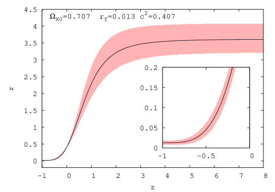
Figure 1: Plot of the ratio $r$ between the energy densities vs. redshift for the best-fit model. As the inset shows, $r_{f}\equiv r(z)$ does not vanish when $z\rightarrow-1$. In this, and the next figure, the red swath indicates the region obtained by including the $1\sigma$ uncertainties of the constrained parameters used in the calculation.

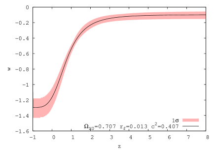
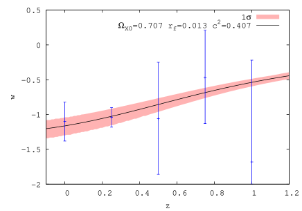
Figure 2: The equation of state parameter vs. redshift up to $z=8$ (left panel), and up to $z=1.2$ only (right panel) for the best fit holographic model. At high redshifts $w$ approaches the equation of state of non-relativistic matter and at low redshifts it does not depart significantly from $-1$. The observational data are taken from [9]. The error bars indicate a $2\sigma$ uncertainty.

2 Contrasting the model with observation

The model has four free parameters ($\Omega_{X0}$, $c^{2}$, $r_{f}$, and $H_{0}$) which we constrained with observational data from supernovae (557 data points [10]), cosmic background radiation [11], baryon acoustic oscillations (at $z=0.35$ [12] and $z=0.2$ [13]), gas mass fraction in galaxy clusters (42 data points from x-ray measurements [14]), the Hubble function history (15 data points [15], [16], [17], and [18]), and the growth function (5 data points from Table 2 in [19]). (See [7] for details).

Data from the growth function -which correspond to matter perturbations within the horizon- are particularly relevant because they can more easily discriminate between cosmological models with a similar history of the Hubble function. For the model under consideration the growth function of matter, $f\equiv d\ln\delta_{M}/d\ln a$, is governed by

$$f^{\prime}+f^{2}+\left(\frac{1}{c^{2}(1+r)}+Q\frac{1+r}{r}\right)f-\frac{3r^{3}+2Q^{2}(1+r)^{3}-2Qr(2+r-r^{2})}{2r^{2}(1+r)}=0\,.$$ (5)

In the non-interacting limit, $Q\rightarrow 0$, this expression reduces to the corresponding one of the Einstein-de Sitter cosmology, namely: $f^{\prime}+f^{2}+[2\,+\,(\dot{H}/H^{2})]f=3\Omega_{M}/2$.

The best-fit values of the free parameters are found to be: $\Omega_{X0}=0.707\pm 0.009$, $c^{2}=0.407^{+0.033}_{-0.028}$, $r_{f}=0.013^{+0.006}_{-0.005}$, and $H_{0}=71.8\pm 2.9$ km/s/Mpc. This together Table 1 and figures 3 and 4 summarizes our findings. It is worthy of note that the non-interacting case, $Q=0$ (which implies $r_{f}=0$ via Eq. (4)), lies over $2\sigma$ away from the best fit value. This seems to be a generic feature of holographic models.

Table 1 shows the partial, total, and total $\chi^{2}$ over the number of degrees of freedom of the holographic model along with the corresponding values for the $\Lambda$CDM model. The latter has just two free parameters, $\Omega_{M0}$ and $H_{0}$. Their best-fit values after constraining the model to the same sets of data are $\Omega_{M0}=0.266\pm 0.006$, and $H_{0}=71.8\pm 1.9\,$km/s/Mpc.

Table 1: $\chi^{2}$ values of the best-fit holographic model and the best fit $\Lambda$CDM model.

Model	$\chi^{2}_{sn}$	$\chi^{2}_{cmb}$	$\chi^{2}_{bao}$	$\chi^{2}_{x-rays}$	$\chi^{2}_{H}$	$\chi^{2}_{gf}$	$\chi^{2}_{{\rm total}}$	$\chi^{2}_{{\rm total}}/dof$
Holographic	$543.70$	$0.01$	$1.20$	$41.79$	$9.57$	1.06	$597.34$	$\;\;0.96$
$\Lambda$CDM	$542.87$	$0.05$	$1.13$	$41.59$	$8.73$	0.43	$594.80$	$\;\;0.96$

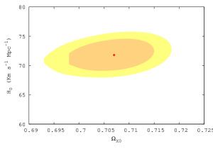
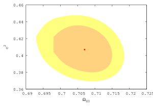
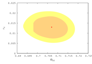
Figure 3: Panels from left to right show the 68.3% and 95.4% confidence contours for the pairs of free parameters ($\Omega_{X0}$, $H_{0}$), ($\Omega_{X0}$, $c^{2}$), ($\Omega_{X0}$, $r_{f}$), respectively, obtained by constraining the holographic model with SN Ia+CMB-shift+ BAO+x-ray+H(z)+growth function data. The solid point in each panel locates the best fit values.

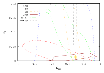
Figure 4: Left panel: Probability contours for SN Ia, CMB, BAO, x-ray, $H(z)$, and growth function, in the ($\Omega_{X0},c^{2}$) plane. The joined constraint uses $\chi^{2}_{\rm total}=\chi^{2}_{sn}\,+\,\chi^{2}_{cmb}\,+\,\chi^{2}_{bao}\,+\,\chi^{2}_{x-rays}+\,\chi^{2}_{Hubble}\,+\,\chi^{2}_{gf}$. Right panel: Idem for the ($\Omega_{X0},r_{f}$) plane.

3 Conclusions

The statistical analysis sketched above shows that the ratio $\chi^{2}_{total}/dof$ is lower than unity for the holographic interacting model of section 1, whereby it is compatible with observation. However, as Table 1 shows, the $\Lambda$CDM model fits better the same sets of data. Yet, the latter cannot explain the cosmic coincidence problem while the former can.

ID was funded by the “Universidad Autónoma de Barcelona" through a PIF fellowship. This research was partly supported by the Spanish Ministry of Science and Innovation under Grant FIS2009-13370-C02-01, and the “Direcció de Recerca de la Generalitat" under Grant 2009SGR-00164.

References

References

- [1] Ng YJ 2001 Phys. Rev. Lett. 86 2946
- [2] Arzano M, Kephart TW and Ng YJ 2007 Phys. Lett. B 649 243
- [3] Zimdahl W and Pavón D 2007 Class. Quantum Grav. 24 5461
- [4] Radicella N and Pavón D 2010 J. Cosmol. Astropart. Phys. JCAP10(2010)005
- [5] Brustein R 2008 “Cosmological Entropy Bounds" in String Theories and Fundamental Interactions (Lecture Notes in Physics vol 737) eds M Gasperini and J Maharana (Heidelberg: Springer) pp 619-659
- [6] Durán I, Pavón D and Zimdahl W 2010 J. Cosmol. Astropart. Phys. JCAP07(2010)018
- [7] Durán I and Pavón D 2011 Phys. Rev. D, in the press (Preprint arXiv:1012.2986 [astro-ph.CO])
- [8] Steinhardt PJ 1997 “Cosmological Challenges for the 21st Century" in Critical Problems in Physics eds VL Fitch at al (Princeton: Princeton University Press) pp 123-146
- [9] Serra P et al 2009 Phys. Rev. D 80 121302
- [10] Amanullah R et al 2010 Astrophys. J. (in the press) Preprint arXiv:1004.1711
- [11] Komatsu E et al 2009 Astrophys. J. Suppl. 180 330
- [12] Eisenstein DJ et al 2005 Astrophys. J. 633 560
- [13] Percival WJ et al 2010 Mon. Not. R. Astron. Soc. 401 2148
- [14] Allen SW et al 2008 Mon. Not. R. Astron. Soc. 383 879
- [15] Riess AG et al 2009 Astrophys. J. 699 539
- [16] Gaztañaga E, Cabré A, and Hui L 2009 Mon. Not. R. Astron. Soc. 399 1663
- [17] Simon J, Verde L and Jiménez R 2005 Phys. Rev. D 71 123001
- [18] Stern D, Jiménez R, Verde L, Kamionkowski M and Stanford SA 2010 J. Cosmol. Astropart. Phys. JCAP02(2010)008
- [19] Gong Y 2008 Phys. Rev. D 78 123010