Instantaneous Gelation in Smoluchowski’s Coagulation Equation Revisited

Abstract

We study the solutions of the Smoluchowski coagulation equation with a regularisation term which removes clusters from the system when their mass exceeds a specified cut-off size, $M$. We focus primarily on collision kernels which would exhibit an instantaneous gelation transition in the absence of any regularisation. Numerical simulations demonstrate that for such kernels with monodisperse initial data, the regularised gelation time decreases as $M$ increases, consistent with the expectation that the gelation time is zero in the unregularised system. This decrease appears to be a logarithmically slow function of $M$, indicating that instantaneously gelling kernels may still be justifiable as physical models despite the fact that they are highly singular in the absence of a cut-off. We also study the case when a source of monomers is introduced in the regularised system. In this case a stationary state is reached. We present a complete analytic description of this regularised stationary state for the model kernel, $K(m_{1},m_{2})=\max\left\{m_{1},m_{2}\right\}^{\nu}$, which gels instantaneously when $M\to\infty$ if $\nu>1$. The stationary cluster size distribution decays as a stretched exponential for small cluster sizes and crosses over to a power law decay with exponent $\nu$ for large cluster sizes. The total particle density in the stationary state slowly vanishes as $(\log(M^{\nu-1}))^{-1/2}$ when $M\to\infty$. The approach to the stationary state is non-trivial : oscillations about the stationary state emerge from the interplay between the monomer injection and the cut-off, $M$, which decay very slowly when $M$ is large. A quantitative analysis of these oscillations is provided for the addition model which describes the situation in which clusters can only grow by absorbing monomers.

I Introduction

The determination of the statistical time evolution of an ensemble of particles undergoing irreversible binary coagulation is a problem which arises in many different contexts in the physical, chemical and biological sciences. See ERN1986 for a list of applications. Of pre-eminent interest is the cluster size distribution, $N_{m}(t)$, which specifies the average density of particles of mass, $m$, at a given time $t$. Often one aims to derive $N_{m}(t)$ from a given model of the microscopic dynamics governing cluster coagulation. This problem has been extensively studied for almost a century starting with the seminal work of Smoluchowski SMO1917 who showed that, at the mean field level, the cluster size distribution of a statistically homogeneous system evolves according to the Smoluchowski coagulation equation:

$$\partial_{t}N_{m} = \int_{0}^{m}dm_{1}K(m_{1},m-m_{1})N_{m_{1}}N_{m-m_{1}}$$

$$- 2N_{m}\int_{0}^{\infty}dm_{1}K(m,m_{1})N_{m_{1}}+\frac{J}{m_{0}}\ \delta(m-m_{0}).$$

Here the coagulation kernel, $K(m_{1},m_{2})$, is proportional to the probability rate for a cluster of mass $m_{1}$ merging with a cluster of mass $m_{2}$. At this level of description, it encodes all relevant information about the underlying micro-physics. $J$ is the rate of injection of monomers, having mass $m_{0}$, into the system. $J$ may be zero depending on the application. In this paper, we take Eq. (I) as our departure point. It is expected to apply when the clusters remain well-mixed (despite aggregation), but the elucidation of the exact conditions under which Eq. (I) is rigorously obtained as the mean field limit of an underlying stochastic process can be a subtle question. Mathematically inclined readers are referred to the review by Aldous ALD1999 for some common mathematical perspectives on this issue. A physical example of a situation in which the applicability of Eq. (I) fails due to the generation of spatial correlations between particles by diffusive fluctuations is discussed in detail in CRZ2006 .

In many applications the microphysics is scale invariant, at least over some range of cluster sizes. That is to say, the coagulation kernel is a homogeneous function of its arguments, the degree of homogeneity of which we shall denote by $\lambda$:

$$K(cm_{1},cm_{2})=c^{\lambda}K(m_{1},m_{2}).$$ (2)

In many cases, such kernels result in solutions of Eq. (I) which exhibit self-similarity. This means that the cluster size distribution asymptotically takes the form $N(m,t)\sim s(t)^{a}F(m/s(t))$ where $s(t)$ is a characteristic cluster size which grows in time, $a$ is a dynamical scaling exponent and $\sim$ denotes the scaling limit: $t\to\infty$ and $m\to\infty$ with $m/s(t)$ fixed. Furthermore, it has been proven for the constant, sum and product kernels that such self-similar solutions are attracting for any initial data with finite $(\lambda+1)^{\mathrm{th}}$ moment MP2004 . Much work in the physics literature on the theory of coagulation, following the work of Van Dongen and Ernst EVD1988 , has focused on the problem of determining the properties of the scaling function $F(x)$ and the exponent $a$ from the scaling properties of $K(m_{1},m_{2})$. An almost complete scaling theory of Eq. (I) is now known. See the review by Leyvraz LEY2003 for a modern discussion.

A key feature of this scaling theory, and one which is of considerable importance for what follows, is the fact that the scaling properties of Eq. (I) are often very sensitive to the rate of coagulation of clusters of widely different masses. In order to parameterise this dependence in a general way, and following the notation of LEY2003 , we introduce the scaling exponents $\mu$ and $\nu$ which specify the asymptotic behaviour of the coagulation kernel in the limit where the mass of one cluster greatly exceeds that of the other:

$$K(m_{1},m_{2})\sim m_{1}^{\mu}m_{2}^{\nu}\ \ m_{1}\!\!\ll\!\!m_{2}.$$ (3)

Clearly from Eq. (2), we must have $\mu+\nu=\lambda$. We shall use the notation $\mathcal{M}_{\alpha}(t)$ to denote the $\alpha$-moment of the cluster size distribution:

$$\mathcal{M}_{\alpha}(t)=\int_{0}^{\infty}m^{\alpha}\,N_{m}(t)\,dm.$$ (4)

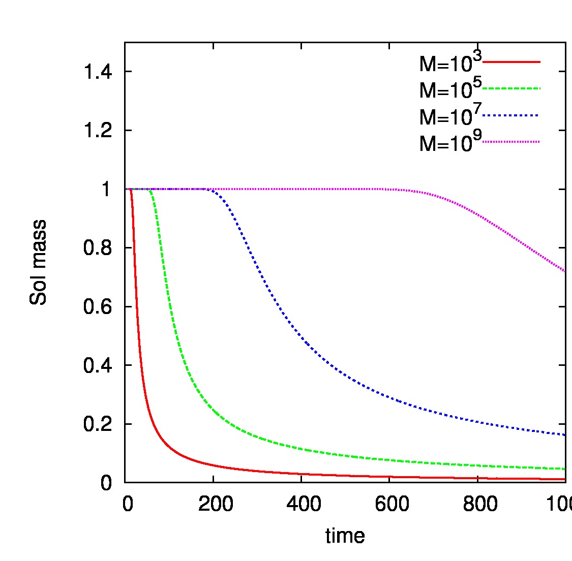
Figure 1: (Color online) Total mass density, $\mathcal{M}_{1}(t)$, for $K(m_{1},m_{2})=(m_{1}m_{2})^{1/4}$.

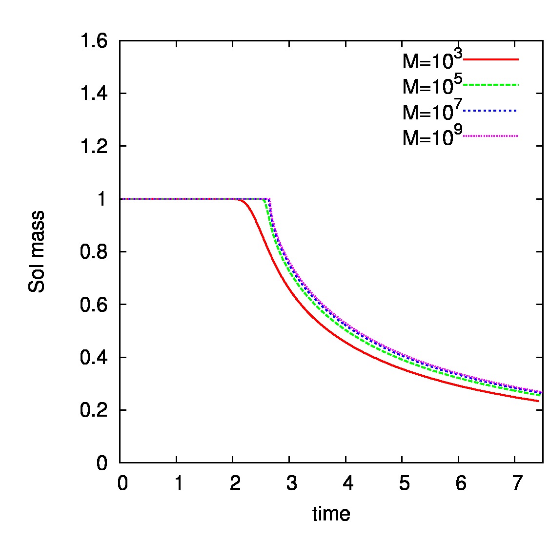
Figure 2: (Color online) Total mass density, $\mathcal{M}_{1}(t)$, for $K(m_{1},m_{2})=(m_{1}m_{2})^{3/4}$.

The first moment, the total mass density, $\mathcal{M}_{1}(t)=\int_{0}^{\infty}m\,N_{m}(t)\,dm$, is governed by conservation of material and is thus formally conserved by Eq. (I) when $J=0$. If $J\neq 0$ we simply have $\mathcal{M}_{1}(t)=\mathcal{M}_{1}(0)+J\,t$. This accords with the intuition imparted by the mass-conserving character of the individual coagulation events. This intuition is challenged, however, by one of the more interesting phenomena to emerge from the scaling theory of the Smoluchowski equation: the so-called gelation transition. Originally conjectured by Lushnikov LUS1977 and Ziff ZIF80 and put on a firmer theoretical footing by Van Dongen and Ernst VDE1986 , gelation refers to the fact that, for kernels having $\lambda>1$, mass-conservation can be spontaneously broken in finite time. That is to say, there exists a time $t^{*}$, known as the gelation time such that

$$\mathcal{M}_{1}(t)<\int_{0}^{\infty}m\,N_{m}(0)\,dm\ \ \mbox{$t>t^{*}$}.$$

The characteristic cluster size, $s(t)$, typically diverges at the gelation time. The “missing” mass can be interpreted as going into a cluster of infinite mass or “gel”. The generation of arbitrarily large clusters in finite time might seem surprising but can be perfectly physical in some cases. One example is polymer gelation in which clusters merge by the formation of crosslinks and therefore do not need to move in order to coalesce. For other examples of kernels having $\lambda>1$, the solution of Eq. (I) describes only the intermediate asymptotics of the underlying physical system over some range of cluster sizes and for times less than the gelation time. Once this intermediate asymptotic range has been identified, there is no conceptual problem with the loss of mass conservation in the Smoluchowski or the generation of infinite clusters. Indeed, the gelation transition has even been observed experimentally, for example in polymer aggregation LNP1990 , and found to exhibit dynamics in reasonable agreement with the predictions of the Smoluchowski equation.

It turns out, however, that this is not the full story. Soon after the discovery of the gelation phenomenon, it was realised by Hendriks, Ernst and Ziff HEZ1983 that the kernel $K(m_{1},m_{2})=(m_{1}m_{2})^{2}$ produced a series expansion for the second moment of the cluster size distribution which seemed to have zero radius of convergence in time. This led the authors to suggest the possibilty of gelation occuring at time $0+$. Detailed study of the scaling properties of the Smoluchowski equation subsequently led to formal arguments VDO1987 , later made rigourous CC1992 , which show that for coagulation kernels having exponent $\nu>1$, the gelation time is actually zero. This surprising phenomenon is referred to as instantaneous gelation. Even more surprisingly, the gelation process can be complete in the sense that $\mathcal{M}_{1}(t)=0$ for $t>0$. See JEO1999 for a mathematical discussion of this point. A situation in which all mass vanishes from the system in time $0+$ clearly cannot describe even the intermediate asymptotics of any physical coagulation problem. For applications such as the coagulation of polymers or colloidal aggregates, the fact that the available surface area of an aggregate cannot grow faster than its volume means that the exponent $\nu$ cannot be greater than 1. If the only applications of the Smoluchowski equation came from polymer science, the phenomenon of instantaneous gelation would be regarded as a mathematical pathology which need not concern physicists. Yet there are models for which it can plausibly be argued that the exponent $\nu$ is greater than 1. One such example is the astrophysical phenomenon of gravitational clustering SW1978 ; KON01 which is thought to play a role in determining the large scale matter distribution of the universe. A second important example is that of differential sedimentation of water droplets falling at their terminal velocity KC2002 ; HNS2008 , one of the processes responsible for the observed droplet size distribution in clouds FFS2002 ; FSV2006 . Furthermore, there are even proposed heuristic solutions of Eq. (I) in the literature for such models KON01 ; HNS2008 which seem reasonably supported by numerical simulations. The question of how this is possible, given the known mathematical results on instantaneous gelation discussed above, is the principal topic of this paper. It should be clear from the outset that the presence of an instantaneous gelation transition for a particular kernel indicates that the underlying physical model omits some process which becomes important for short timescales or for large masses. For example, in the case of droplet coalescence in clouds, the Stokes assumption for the terminal velocity of a droplet is ultimately responsible for the exponent $\nu$ exceeding 1. This assumption ceases to be valid for sufficiently large droplets (see KC2002 and the references therein).

II Instantaneous Gelation in the Regularised System

The gelation phenomenon in particle systems is best understood by considering a regularisation of the system and studying the behaviour as this regularisation is removed. Two natural regularisations can be found in the literature. One approach is to consider the stochastic dynamics of a finite number of particles as has been done by Lushnikov LUS2005 for the product kernel. Another approach is to introduce a mass cut-off, $M$, into the Smoluchowski equation. This has been done by Filbet and Laurençot FL2004 . These are different regularisations but both show singular behaviour as the regularisation is removed when $\lambda>1$.

In this paper, we regularise by the latter method. As in FL2004 , the cut-off is introduced in such a way that clusters having mass $m>M$ are removed from the system:

$$\partial_{t}N_{m} = \frac{1}{2}\,\int_{1}^{m}dm_{1}K(m_{1},m-m_{1})N_{m_{1}}N_{m-m_{1}}$$

$$- N_{m}\int_{1}^{M-m}dm_{1}K(m,m_{1})N_{m_{1}}+J\ \delta(m-1)$$

$$- D_{M}\left[N_{m}(t)\right]$$

where

$$D_{M}\left[N_{m}(t)\right]=N_{m}\int_{M-m}^{M}dm_{1}\,K(m,m_{1})\,N_{m_{1}}$$ (6)

describes the removal of clusters having $m>M$. This regularisation explicitly breaks mass conservation. Furthermore, we shall implicitly measure all masses in terms of the monomer mass from now on so that the lower cut-off, $m_{0}$, is set equal to 1. Clearly this is not the only way in which the problem can be regularised. In particular, by omitting $D_{M}\left[N_{m}(t)\right]$ from Eq. (II) one would obtain an explicitly conservative regularisation. One would expect the behaviour to be completely different in this case. The differences between conservative and non-conservative regularisations for a related aggregation–fragmentation model arising in the kinetics of waves are explored in CON2009 . The fact that the gelation transition involves a loss of mass from the system suggests that the non-conservative regularisation is more natural. While we implement this regularisation as a hard cut-off, $M$, we would expect the behaviour described below to be qualitatively the same for smoother regularisations provided that the non-conservative property is retained.

Figs. 1 and 2 show the mass contained in this regularised system as a function of time for a sequence of values of $M$ for the non-gelling kernel $K(m_{1},m_{2})=(m_{1}m_{2})^{1/4}$ (Fig. 1) and for the gelling kernel $K(m_{1},m_{2})=(m_{1}m_{2})^{3/4}$ (Fig. 2). These were obtained by numerical solution of Eq. (II) with monodisperse initial data.

All numerical results in this paper were obtained using the algorithm developed by Lee in LEE2000 ; LEE2001 . This algorithm involves coarse-graining the masses into bins whose width increases exponentially with mass and then using the Smoluchowski equation to approximate the mass transferred per timestep as a result of the aggregation of clusters in each pair of bins. The approximation explicitly enforces mass conservation. Full details of the coarse-graining and formulae for the computation of mass transfer are provided in LEE2000 . In a slight modification of Lee’s algorithm, the regularisation described by Eq. (6) is implemented by introducing an infinite width bin, $\left[M,\infty\right]$, which accumulates any mass transferred to clusters larger than $M$. We also modified the timestepping procedure, replacing Lee’s original explicit timestepping method with an adaptive implicit trapezoidal rule. This is essential because the Smoluchowski equation becomes increasingly stiff for larger values of $\lambda$ to the extent that the results presented here could not be obtained with explicit timestepping. The implicit trapezoidal rule requires the solution of a set of nonlinear equations at each timestep which was done using the GSL GSL implementation of the Rosenbrock algorithm ROS1960 . Explicit formulae and further discussion of these modifications of Lee’s algorithm can be found in CON2009 .

We see that for the non-gelling system, mass conservation is restored in the limit $M\to\infty$ whereas for the gelling system, it is not. This latter situation will be recognisable to readers familiar with the theory of turbulence where it is widely believed that energy conservation is not restored when the limit of zero viscosity is taken in the Navier-Stokes equations FRI1995 , a phenomenon referred to as the dissipative anomaly. A similar phenomenon is observed in the kinetics of wave turbulence CON2009 . There is no physical contradiction in the fact that mass conservation is broken in the Smoluchowski equation in the gelling regime. It simply means that for times larger than the gelation time, the underlying conservative coagulation dynamics must be modified for the largest clusters.

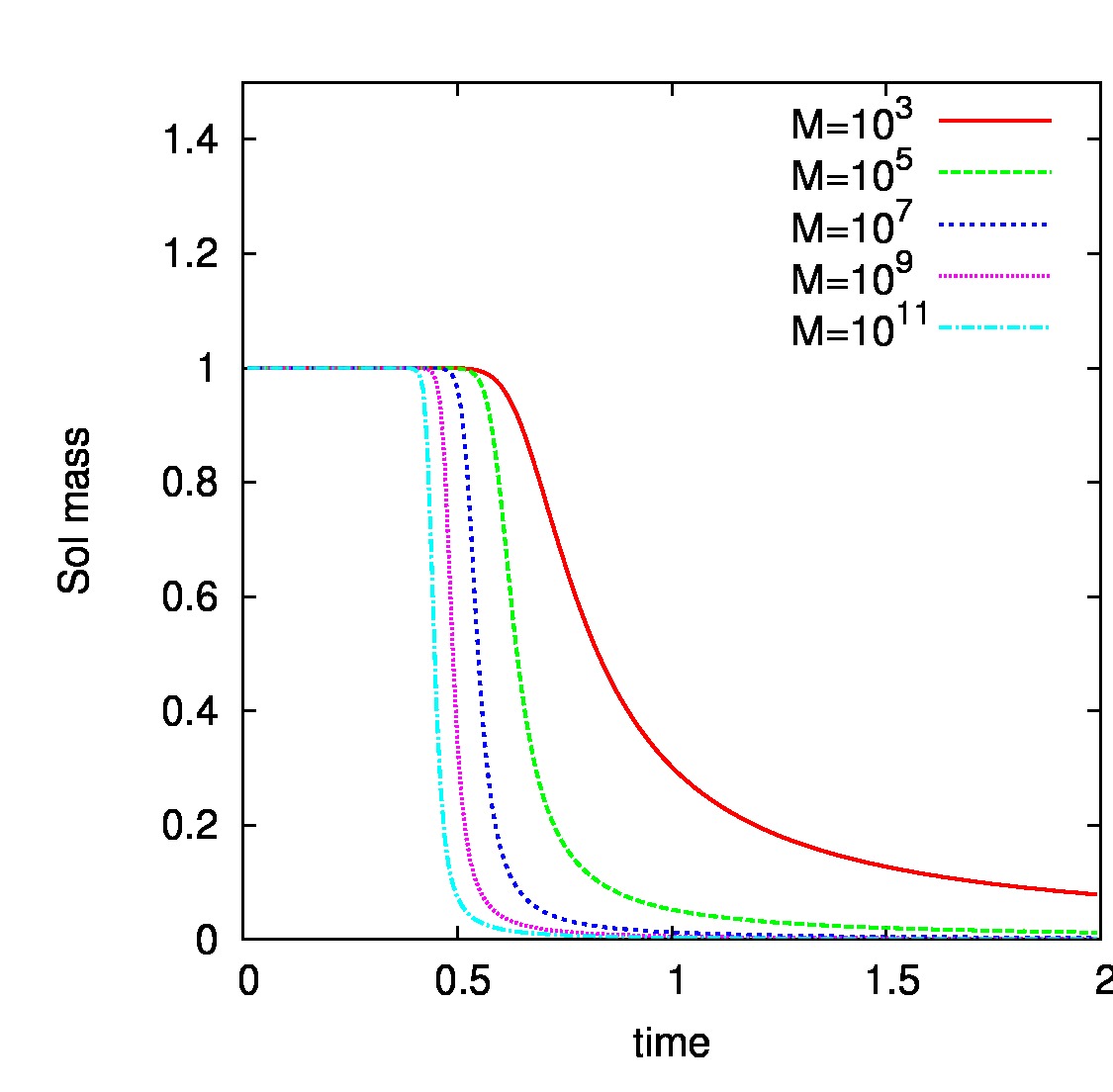
Figure 3: (Color online) Total mass density, $\mathcal{M}_{1}(t)$, for the generalised sum kernel, $K(m_{1},m_{2})=m_{1}^{\frac{3}{2}}+m_{2}^{\frac{3}{2}}$.

Let us now consider what happens when an instantaneously gelling kernel is inserted into the regularised Smoluchowski equation. An archetypal instantaneously gelling kernel, which we shall use extensively in what follows, is the generalised sum kernel:

$$K_{\epsilon}(m_{1},m_{2})=m_{1}^{1+\epsilon}+m_{2}^{1+\epsilon}.$$ (7)

For this kernel $\lambda=\nu=1+\epsilon$ and $\mu=0$. According to the classification of Van Dongen and Ernst, it is nongelling for $\epsilon<0$ and instantaneously gelling for $\epsilon>0$. In the marginal case, $\epsilon=0$, it is the simple sum kernel which is exactly solvable, at least in the absence of a source of mononers LEY2003 , and turns out to be non-gelling. Fig. 3 shows the sol mass in the regularised system with the generalised sum kernel with $\epsilon=\frac{1}{2}$ for a sequence of increasing values of the regularisation mass, $M$. In the presence of the cut-off, the regularized gelation time, $t^{*}_{M}>0$, is clearly identifiable. This regularised gelation time, although finite, decreases as $M_{\mathrm{m}ax}$ increases. Extrapolating the behaviour seen in Fig. 3, it is plausible that the gelation time vanishes as $M\to\infty$ consistent with the expectation that the unregularised system exhibits complete instantaneous gelation. Instantaneous gelation has not, to the best of our knowledge, been successfully numerically demonstrated in the literature previously. In the most extensive numerical study of the Smoluchowski equation to date, that of Lee LEE2001 , the numerical difficulties posed by kernels like Eq. (7) were explored and it was concluded that there are no self-consistent solutions of Eq. (I) for such kernels. Our results demonstrate that the non-conservative regularisation, Eq. (II), provides one way around these difficulties, at least numerically, although we expect that the regularisation could also be useful for rigorous mathematical studies.

From a physical point of view, the most important observation about the results presented in Fig. 3 is that the regularised gelation time decreases extremely slowly as the cut-off is increased. $t^{*}_{M}$ decreases by a factor of less than 2 as $M$ is increased by 8 orders of magnitude. This very weak dependence means that, in practice, kernels which would exhibit instantaneous gelation, even complete instantateous gelation, for $M=\infty$, can still have smooth, physically reasonable behaviour for finite $M$. The regularised gelation time, $t^{*}_{M}$, depends sufficiently weakly on the actual value of $M$ that such regularised systems may still be useful in modelling. On the basis of our numerics, we conjecture that as $M\to\infty$, the regularised gelation time decreases as $t^{*}_{M}\sim(\log M)^{-\alpha}$ for some $\alpha>0$. This would complement heuristic arguments put forward by Ben-Naim and Krapivsky BNK2003 for gelation in finite systems of particles undergoing exchange-driven growth for which it is argued that the gelation time decreases as a power of the logarithm of the initial number of particles when the aggregation rate increases sufficiently quickly as a function of the mass of the larger cluster and thus becomes instantaneous in the limit of an infinite number of initial particles. An important question, which is left open, is to develop an analytic approach allowing the determination of the functional dependence of $t^{*}_{M_{\mathrm{max}}}$ on $M_{\mathrm{max}}$ and the value of $\alpha$ if the dependence conjectured above in indeed correct. We feel it is unlikely that the numerics can be extended to sufficiently large values of $M_{\mathrm{max}}$ to determine this dependence unambiguously although on the basis of the numerics we have available and taking into account the analytic work on the corresponding problem with a source of monomers reported below, we would not be surprised if $\alpha=1/2$.

We devote much of the remainder of the paper to studing what happens when a source of monomers is introduced into a system with an instantaneously gelling kernel. Such a situation has been partially analysed by Kontorovich KON01 in the context of gravitational clustering and by Horvai et al. HNS2008 in the context of differential sedimentation. Both studies concluded that the system should reach a stationary state at large times in which injection of monomers is balanced by the aggregation of smaller clusters into larger ones (a mass “cascade”). In both cases, the cascade is non-local in the sense that the transfer of mass from small clusters to large is dominated by the interaction of very large and very small clusters. For a detailed discussion of the criteria for locality of mass transfer in cascade solutions of the Smoluchowski equation see CRZ2004 .

III The addition model: a simplified description of runaway absorption of small clusters by large ones

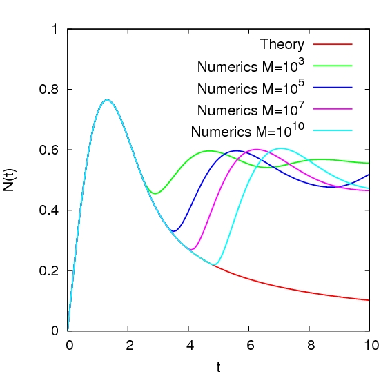
Figure 4: (Color online) Total particle density, $\mathcal{M}_{0}(t)=\int_{0}^{\infty}N_{m}(t)\,dm$ for $K(m_{1},m_{2})=m_{1}+m_{2}$ and source.

Instantaneous gelation is driven by the runaway absorption of small clusters by large ones. This fact is most easily seen from the analytically tractable (but non-gelling) marginal kernel, $m_{1}+m_{2}$, with source of monomers. For $\epsilon=0$, the kernel in Eq.(7) is the standard sum kernel. In this case, integrating Eq.(I) with respect to $m$ (we have set $m_{0}=1$) allows us to obtain the following equation for the total number of particles in the system:

$$\frac{dN}{dt}=-2\mathcal{M}_{1}(t)N(t)+J.$$ (8)

There is no gelation transition at finite time in this case so $\mathcal{M}_{1}(t)=Jt$ and we get a closed equation for $N(t)$:

$$\frac{dN}{dt}=-2JtN(t)+J.$$ (9)

The solution is

$$N(t)=\frac{1}{2}\sqrt{J\pi}\ {\mathrm{Erfi}}(\sqrt{J}\,t)\ {\mathrm{e}}^{-gJt^{2}},$$ (10)

where $\mathrm{Erfi}(x)=-\frac{2i}{\sqrt{\pi}}\int_{0}^{ix}\mathrm{e}^{-y^{2}}dy$ is the “imaginary error function”. This formula shows an interesting feature which is surprising at first sight: while the total number of particles in the system initially increases as we add particles, it subsequently reaches a maximum and starts to decrease as shown in Fig. 4. It tends to zero ($\asymp 1/t$) as time gets large. Meanwhile the total mass in the system increases linearly. This tells us that the long time behaviour of the system is dominated by an ever decreasing number of increasingly massive particles which immediately eat all the monomers injected into the system. Thus we already see the essential feature of non-local interactions at the level of the sum kernel. Fig. 4 demonstrates this behaviour. The numerical solution follows the analytic prediction, Eq. (10), for longer and longer times as the mass cut-off $M$ is increased. This case is marginal in the sense that there is no finite time gelation even though all the mass gets concentrated in larger and larger clusters. If $\epsilon>0$, and the exponent $\nu>1$, then big clusters are so “hungry” that they consume all smaller clusters at a rate which diverges with the cut-off, $M_{\mathrm{max}}$.

The dynamics of a coagulation system dominated by the absorption of small clusters by large ones is modelled in extremis by the so-called “addition model” (Brilliantov & Krapivsky BK1991 ) in which clusters are only permitted to grow by reacting with monomers. Many of the interesting phenomena which we observe in the full coagulation problem have qualitative analogues for the addition model so we shall devote some time to studying it. The addition model corresponds to the kernel

$$K(m_{1},m_{2})=\frac{1}{2}\left(\kappa(m_{1})\,\delta(m_{2}-1)+\kappa(m_{2})\,\delta(m_{1}-1)\right),$$ (11)

where the function $\kappa(m)$ is typically taken to be a homogeneous function of degree $\nu$. This considerably simplifies the coagulation dynamics. Although the addition model can be analyzed for a fairly general set of gelling reaction rates $\{\kappa(m)\}_{m\geq 1}$, we will use the following example for illustrative purposes:

$$\kappa(m)=\left\{\begin{array}[]{ll}\gamma&m=1\\ m^{1+\epsilon},&m=1,2,\ldots,M,~{}\epsilon>0.\end{array}\right.$$ (14)

Here we have changed notation slightly and written $\nu=1+\epsilon$ so that the instantanenous gelation regime corresponds to $\epsilon>0$. The reason for introducing a separate parameter, $\gamma$, to describe the monomer reaction rate will become clear in Sec. VI where we show that by choosing $\gamma$ appropriately, it is possible to make the connection between the addition model and the Smoluchowski equation more quantitative. We shall also impose the initial condition

$$N_{m}(t)=N_{0}\delta_{m,1},$$ (15)

excluding the possibility of zero initial momomer concentration (this is to regularize a change of time to be defined below).

Insertion of Eqs. (11) and (14) into Eq. (I) yields the discrete set of equations

$$\frac{dN_{1}}{dt}(t) = -2\,\gamma\,N_{1}^{2}-\sum_{m=2}^{M}\kappa(m)N_{1}N_{m}+J,$$ (16)

$$\frac{dN_{m}}{dt}(t) = \kappa(m-1)N_{1}N_{m-1}-\kappa(m)N_{1}N_{m}$$ (17)

$$~{}2\leq m\leq M,$$

where explicit dependence of the $N_{m}$ on $t$ has been suppressed for brevity and a cut-off, $M$, has been introduced. Instantaneous gelation in the addition model without a cut-off for $\nu>1$ in the absence of a source was conjectured in BK1991 and subsequently proven by Laurencot LAU1999 providing support for our intuition that the process of aggregation of monomers by large particles is a runaway process in the full aggregation equation when $\nu>1$. Before continuing, we would like to emphasise again that we only expect the addition model to be similar to the Smoluchowski dynamics in the instantaneously gelling regime when the dynamics is dominated by the aggregation of large clusters and monomers. It is known that the addition model has very different dynamics to the Smoluchowski equation in the non-gelling regime, $\nu<1$. In particular it does not exhibit scaling in the absence of a source BK1991 .

Eqs. (16, 17) simplify after a non-linear change of physical time to “monomer” time $\tau$ defined as follows:

$$d\tau(t) = N_{1}(t)dt,$$ (18)

$$\tau(0) = 0.$$ (19)

Once the solution parameterized by the monomer time has been found, the inverse map to the physical time is given by

$$t(\tau)=\int_{0}^{\tau}\frac{d\tau^{\prime}}{N_{1}(\tau^{\prime})}$$ (20)

This integral is proper at $\tau=0$ due to the initial condition, Eq. (15). In terms of the monomer time, Eqs. (16, 17) take the following form:

$$N_{1}^{\prime}(\tau) = -2\,\gamma\,N_{1}(\tau)-\sum_{m=2}^{M}\kappa(m)N_{m}+\frac{J}{N_{1}},$$ (21)

$$N_{m}^{\prime}(\tau) = \kappa(m-1)N_{m-1}-\kappa(m)N_{m},$$ (22)

$$~{}2\leq m\leq M,$$

where ^′ denotes the monomer time derivative $\frac{d}{d\tau}$. Note that Eq. (22) is an inhomogeneous linear system of ODE’s with the inhomogeneity being a nonlinear function of the monomer concentration $N_{1}(\tau)$. It can be solved with respect to the concentrations of polymers using the Laplace transform in the monomer time. The solution can be written in the form

$$N_{m}(\tau) = \int_{0}^{\infty}d\tau^{\prime}K_{m}(\tau-\tau^{\prime})N_{1}(\tau^{\prime}),$$ (23)

$$m=1,2,\ldots,M,$$

where

$$K_{m}(\tau)=\gamma\,\kappa(m)^{-1}\int_{\Gamma}\frac{d\omega}{2\pi}e^{\omega\tau}\prod_{k=2}^{m}\frac{1}{1+\frac{\omega}{\kappa(k)}},$$ (24)

the integration contour $\Gamma=(\sigma-i\infty,\sigma+i\infty)$, and $\sigma$ is a real constant: $\sigma>-\min_{m\geq 2}[\kappa(m)]$. It is easy to see from Eq. (24) that

$$K(\tau)=0,~{}\tau<0,$$

which is an expression of causality in the addition model. Substituting (23) in (21) we arrive at a nonlinear integral equation for the monomer concentration:

$$N_{1}^{\prime}(\tau) = -2\,\gamma\,N_{1}(\tau)-\kappa(1)\,\int_{0}^{\tau}d\tau^{\prime}Q_{M}(\tau-\tau^{\prime})N_{1}(\tau^{\prime})$$ (25)

$$+\frac{J}{N_{1}(\tau)},$$

where

$$Q_{M}(\tau)=\sum_{m=2}^{M}\int_{\Gamma}\frac{d\omega}{2\pi}e^{\omega\tau}\prod_{k=2}^{m}\frac{1}{1+\frac{\omega}{\kappa(k)}}$$ (26)

It is clear from Eq. (25) that $N_{1}(\tau)$ stays positive at all times. The transformation to monomer time is therefore well defined. To find the steady state solution of Eq. (25) we note that all the poles in the integrand of Eq. (26) have negative real parts. Thus,

$$\lim_{\tau\rightarrow\infty}\int_{\tau}d\tau^{\prime}Q_{M}(\tau-\tau^{\prime})N_{1}(\tau^{\prime})=N_{1}(\infty)\int_{0}^{\infty}d\tau Q_{M}(\tau).$$

Substituting this answer into Eq. (25) and setting $N^{\prime}(\infty)=0$ we find that

$$N_{1}(\infty) = \sqrt{\frac{J}{\gamma\left(2+\int_{0}^{\infty}Q_{M}(\tau)\,d\tau\right)}}$$ (27)

$$= \sqrt{\frac{J}{\gamma\,\left(M+1\right)}},$$

where the last equality results from direct integration of the kernel, Eq. (26), over time using Cauchy’s theorem. For the specific case of the kernel, Eq. (14), the corresponding steady state answer for the polymer concentrations is

$$N_{m}(\infty) = \gamma\,N_{1}(\infty)\,\kappa(m)^{-1}$$ (28)

$$= \sqrt{\gamma}\,\sqrt{\frac{J}{M+1}}\,m^{-1-\epsilon}.$$

We acknowledge that it would be easier to find the steady state directly from Eqs. (16, 17), but Eq. (25) will be better suited to study the time evolution in what follows.

IV The full coagulation problem with $\nu>1$ in the presence of a source of monomers

In the presence of a source of monomers, Eq. (I) has a formal stationary solution which scales for large masses as $N_{m}\sim m^{-\frac{\lambda+3}{2}}$ which describes a cascade of mass from small masses to large CRZ2004 . This solution is only valid if the collision integral is convergent. For the case of the kernel Eq. (7), this convergence criterion fails for $\epsilon>0$ CRZ2004 presumably reflecting the tendency for the system to gel instantaneously in this regime. When a cut-off is introduced, a stationary state may be reached if a source of monomers is present although this stationary state must involve the cut-off rather than being of the cascade type. In HNS2008 such a stationary state was found for the case of differential sedimentation ($\nu=\frac{4}{3}$) which scaled for large masses as $N_{m}\sim m^{-\frac{4}{3}}$.

In this section we perform a systematic analysis of the stationary state for the model kernel

$$K(m_{1},m_{2})=\mathrm{max}(m_{1},m_{2})^{\nu},$$ (29)

which captures the essential features of instantaneously gelling systems while permitting some convenient simplifications of the equations. If we assume that the system reaches a stationary state and define

$$\Gamma_{M}=\sum_{m=1}^{M}m^{\nu}N_{m},$$ (30)

then some manipulations of the discrete analogue of Eq. (I) show that the stationary state can be expressed via a recursion relation:

$$N_{m}=\frac{\frac{1}{2}\sum_{p=1}^{m-1}\max(p,m-p)^{\nu}N_{p}N_{m-p}}{\Gamma_{M}+\sum_{p=1}^{m-1}\left(m^{\nu}-p^{\nu}\right)N_{p}}.$$ (31)

which can be iterated to find $N_{m}$ once one observes that the monomer concentration is fixed in the stationary state as:

$$N_{1}=\frac{J}{\Gamma_{M}}$$ (32)

For each value of $M$, this iteration procedure can, in principle, be used to self-consistently determine $\Gamma_{M}$. In this paper, we adopt a different approach which is based on the assumption that the mass transfer is nonlocal in mass space. Following the approach of HNS2008 , Eq. (I) can be approximated by:

$$\frac{\partial N_{m}}{\partial t}=-\mathcal{M}_{1}\frac{\partial}{\partial m}\left(m^{\nu}N_{m}\right)-\mathcal{M}_{\nu}\,N_{m}$$ (33)

where the moments $\mathcal{M}_{1}$ and $M_{\nu}$ are now to be computed with the cut-off retained:

$$\mathcal{M}_{\alpha}=\int_{1}^{M}m^{\alpha}\,N_{m}\,dm.$$ (34)

The source and sink terms have been omitted for now. In obtaining Eq. (33) it has been assumed that the integrals $\mathcal{M}_{1}$ and $\mathcal{M}_{\nu}$ are dominated by their lower and upper limits of integration respectively. The consistency of this assumption will be determined a-posteriori. Since $\mathcal{M}_{1}$ and $\mathcal{M}_{\nu}$ do not depend on $m$, Eq. (33) has the stationary solution:

$$N_{m}=C\,\exp\left[\beta\frac{m^{1-\nu}}{\nu-1}\right]\,m^{-\nu},$$ (35)

where $C$ is an arbitrary constant and we have, for convenience, introduced the parameter,

$$\beta=\frac{\mathcal{M}_{\nu}}{\mathcal{M}_{1}}.$$ (36)

Although we do not know the value of $\beta$ a-priori, it can now be determined self-consistently due to the fact that, when $N_{m}$ is given by Eq.(35), the integrals $\mathcal{M}_{1}$ and $\mathcal{M}_{\nu}$ can be expressed explicitly in terms of incomplete gamma functions:

$$\mathcal{M}_{1}(\beta) = \frac{C}{\nu-1}\left(\frac{1-\nu}{\beta}\right)^{\frac{\nu-2}{\nu-1}}\left[\Gamma\left(\frac{\nu-2}{\nu-1},-\frac{\beta\,M^{1-\nu}}{\nu-1}\right)-\Gamma\left(\frac{\nu-2}{\nu-1},-\frac{\beta}{\nu-1}\right)\right]$$ (37)

$$\mathcal{M}_{\nu}(\beta) = \frac{C}{\nu-1}\left(\frac{1-\nu}{\beta}\right)^{\frac{1}{1-\nu}}\left[\Gamma\left(\frac{1}{1-\nu},-\frac{\beta\,M^{1-\nu}}{\nu-1}\right)-\Gamma\left(\frac{1}{1-\nu},-\frac{\beta}{\nu-1}\right)\right].$$ (38)

After some algebra, Eq. (36) reduces to the following consistency condition for the value of $\beta$:

$$\Gamma\left(\frac{\nu-2}{\nu-1},-\frac{\beta\,M^{1-\nu}}{\nu-1}\right)-\Gamma\left(\frac{\nu-2}{\nu-1},-\frac{\beta}{\nu-1}\right)=-\frac{1}{\nu-1}\,\Gamma\left(\frac{1}{1-\nu},-\frac{\beta\,M^{1-\nu}}{\nu-1}\right)+\frac{1}{\nu-1}\,\Gamma\left(\frac{1}{1-\nu},-\frac{\beta}{\nu-1}\right)$$ (39)

Given $\nu>1$, this can be solved numerically for any value of $M$. Such a numerical investigation indicates that $\beta$ is a slowly increasing function of $M$. Furthermore, since we expect the integrals $\mathcal{M}_{1}$ and $\mathcal{M}_{\nu}$ to be dominated by their respective lower and upper limits of integration as $M\to\infty$, we would expect Eq. (39) to satisfy the following asymptotic balance for large $M$:

$$-\Gamma\left(\frac{\nu-2}{\nu-1},-\frac{\beta}{\nu-1}\right)\sim-\frac{1}{\nu-1}\,\Gamma\left(\frac{1}{1-\nu},-\frac{\beta\,M^{1-\nu}}{\nu-1}\right).$$ (40)

Since numerics indicate that $\beta$ increases (but only slowly) as $M$ grows and $\nu>1$, the argument of the left-hand gamma function, $\frac{\beta}{\nu-1}$, should increase in the limit of interest. Likewise, the argument of the right-hand gamma function, $\frac{\beta\,M^{1-\nu}}{\nu-1}$, should decrease in the limit of interest. The relevant leading order asymptotics are then:

$$\Gamma(a,z) \sim z^{a-1}\,e^{-z} z\to\infty$$ as (41)

$$\Gamma(a,z) \sim-\frac{1}{a}\,z^{a} \mbox{as $z\to 0$}.$$ (42)

Substituting these into Eq. (40), one finds that the leading order terms balance as $M\to\infty$ provided

$$\beta\sim\log(M^{\nu-1}).$$ (43)

Whilst the index $\nu-1$ could be absorbed within the implied front factor in $\beta$, we keep it in the following expressions since it captures how the dependence on the cut-off, $M$, goes away when $\nu$ approaches unity. Knowing $\beta$, Eqs. (42) and (41) can now be used to detemine the asymptotic behaviour of $\mathcal{M}_{1}$ and $\mathcal{M}_{\nu}$ from Eqs. (37) and (38). After some work one finds:

$$\mathcal{M}_{1}\sim\frac{CM}{\log(M^{\nu-1})} M\to\infty$$ as (44)

$$\mathcal{M}_{\nu}\sim C\,M \mbox{as $M\to\infty$}.$$ (45)

It now remains to determine the constant $C$ in Eq. (35) in order to close the argument and allow us to check for consistency. This can be done using global mass balance. Multiplying Eq. (II) (with the kernel Eq. (29)) by $m$ and integrating from 1 to $M$ yields the global mass balance condition:

$$J=\int_{1}^{M}dm\ m\,N_{m}\int_{M-m}^{M}dm_{1}\ m_{1}^{\nu}N_{m_{1}}.$$ (46)

Our assumption of nonlocality allows to replace the inner integral by $\mathcal{M}_{\nu}$ in the limit of large $M$ since it is dominated by its upper limit. Consequently the global mass balance condition in the limit of large $M$ is

$$J=\mathcal{M}_{1}\,\mathcal{M}_{\nu}=\frac{C^{2}M^{2}}{\log(M^{\nu-1})},$$ (47)

where we have used Eqs. (44) and (45). This gives

$$C=\frac{\sqrt{J\log(M^{\nu-1})}}{M}.$$ (48)

Putting this all together with Eq. (35) the asymptotic solution of Eq. (33) is

$$N_{m}=\frac{\sqrt{J\,\log(M^{\nu-1})}}{M}\,M^{m^{1-\nu}}\,m^{-\nu}.$$ (49)

Everything becomes self-consistent: $\mathcal{M}_{1}$ becomes independent of $M$ and $\mathcal{M}_{\nu}$ diverges as $\sqrt{\log(M^{\nu-1})}$ when $M$ gets large thereby justifying the use of Eq. (33). This theory does a good job of capturing the general features of the stationary state: stretched exponential decay at small cluster sizes followed by a cross-over to a power law decay with exponent $\nu$ for large cluster sizes but with an amplitude which decreases with the cut-off, $M$. Fig. 5 compares Eq. (49) with the stationary state obtained from numerical simulations of Eq. (II) with $\nu=3/2$ for a range of values of $M$. The agreement is excellent given that there are no adjustable parameters in Eq. (49). Note that the large mass behaviour, $N_{m}\sim m^{-\nu}$, is in agreement with the stationary solution of the addition model, Eq. (28), obtained in Sec. III.

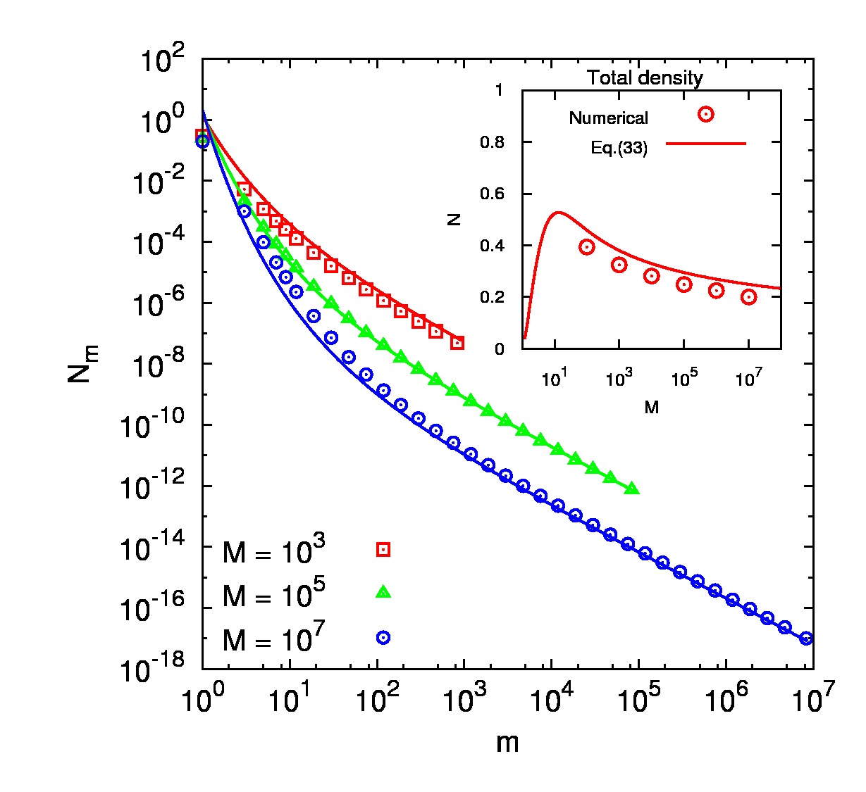
Figure 5: (Color online) Non-local stationary state (theory vs numerics) for $\nu=3/2$.

Finally, we can now quantify the rate at which the system becomes singular as the cut-off, $M$, is increased. Using Eq. (49) to calculate the total particle density in the stationary state we get

$$N=\frac{\sqrt{J}\left(M-M^{M^{1-\nu}}\right)}{M\,\sqrt{\log(M^{\nu-1})}}\sim\sqrt{\frac{J}{\log(M^{\nu-1})}}\ \ \mbox{as $M\to\infty$}.$$ (50)

The density of particles in the stationary state thus vanishes as the cut-off is removed which is the signature of instantaneous gelation. The approach to zero is logarithmically slow however. The asymptotic estimate, Eq. (50), is compared against the total density measured from a sequence of numerical simulations with $\nu=3/2$ and different values of the cut-off in the inset of Fig. 5. The theory again produces convincing agreement with numerics without any adjustable parameters.

V Approach to the Stationary State

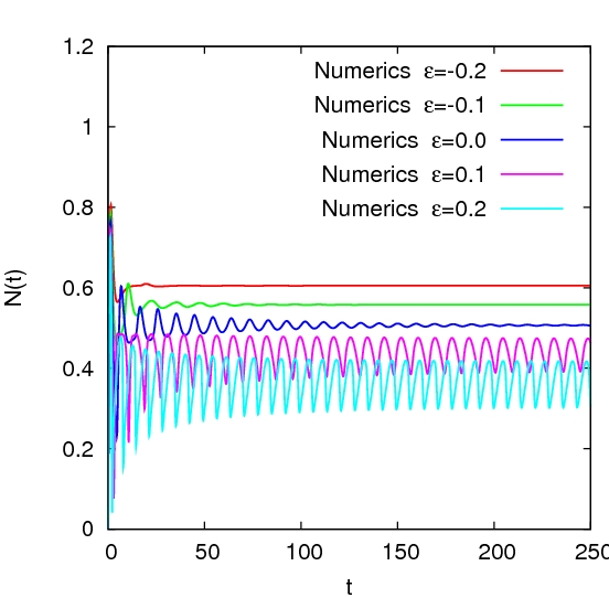
Figure 6: (Color online) Total density vs time for $K(m_{1},m_{2})=m_{1}^{1+\epsilon}+m_{2}^{1+\epsilon}$.

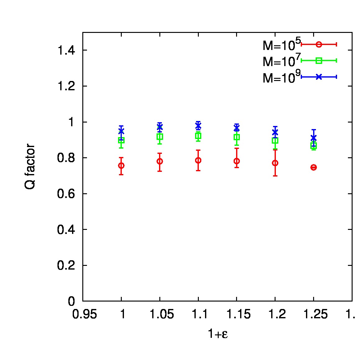
Figure 7: (Color online) “Q-factor” of the oscillatory transient for a range of values of $\nu=1+\epsilon$ and a range of cut-offs, $M$.

Numerical simulations indicate that the approach to the stationary state is interesting. Fig. 6 shows a plot of the total density in the system as a function of time for the generalised sum kernel, Eq. (7), for a range of values of $\epsilon$ with cut-off $M=10^{9}$. In the nonlocal regime, $\epsilon>0$, the approach to the stationary state is characterised by long-lived transient oscillations of the density in the system. This is surprising since there is nothing of an oscillatory or cyclic character in the underlying coagulation dynamics. We note, however, that long-lived oscillations of the total droplet density have been observed in experiments on the phase separation of binary mixtures with nucleation and coagulation of droplets VAV2007 ; BV2010 which may be related to the effect noted here. From Fig. 6, it is not obvious that these oscillations are decaying at all for $\epsilon>0$. From our numerical investigations we believe that these oscillations are indeed transient although the rate of decay becomes very slow as the cut-off is increased. Although the oscillations are quite nonlinear in character, we defined a quantity analogous to the Q-factor of a linear oscillator by measuring the ratio of subsequent maxima of the signal and defining the Q-factor to be the estimated numerical limit of this ratio as $t\to\infty$ (for all of our numerical experiments with $\epsilon>0$, we found that this ratio does indeed seem to converge to a finite value). Thus a Q-factor of 1 would correspond to persistent oscillations.

A summary of these numerical experiments is presented in Fig. 7 which shows numerically estimated Q-factors for the oscillations observed for a range of values of $\epsilon$ and $M$. The most evident trend from the data is the fact that the oscillations come closer and closer to a Q-factor of 1 as $M$ is increased. These measurements indicate that the oscillations are decaying in all cases but only very slowly when the cut-off becomes large. The behaviour as a function of $\epsilon$ is less clear with some possible evidence for a weak maximum.

We offer the following heuristic explanation for how oscillations can be generated in this system. For $\epsilon>0$, the case for which instantaneous gelation should occur in the absence of a cut-off, the indication of Fig. 3 is that the particle density drops close to zero in finite time (but this time is not zero). When monomers are injected into the system, until the cut-off is felt, the mass in the system just increases linearly. However, as soon as large particles are generated, their absorption of the monomers is a runaway process which very rapidly converts the monomers which have accumulated in the system into large particles which are immediately removed by the cut-off. This then resets the system close to its initial state in which there are almost no particles in the system. The dynamics then repeats.

VI Approach to the stationary state in the addition model

We do not, as yet, have an analytic characterisation of the oscillations described in the previous section. Instead, we conclude this article with an analysis of the analogous problem for the simpler case of the addition model discussed in Sec. III for which the oscillatory approach to the stationary state, Eq. (28), can be derived.

The addition model aims to model the most important contribution to the dynamics of the full aggregation model with non-local kernels by concentrating on interactions between “light” and “heavy” particles only. At the level of modeling, there is no reason to expect that the parameters of the addition model are the same as the analogous parameters in the full model. Before proceeding with calculations, we first present a semi-heuristic argument for the most appropriate choice of parameters. Let us first clarify what is meant by “light” and “heavy” in terms of the steady state of the full model, Eq. (49). Heavy particles have masses in the polynomial tail of Eq. (49), $m\gg\log(M)^{\nu-1}$. Light particles belong to the stretched exponential region of Eq. (49), $m\ll\log(M)^{\nu-1}$. Therefore, neglecting logarithmic corrections, we can treat all light particles as effective monomers. Hence, the parameters $J$ and $\kappa_{m}$ for $m>1$ in the addition model are the same as in the full model, but the parameter $\gamma=\kappa(1)$ should be chosen as an effective interaction rate of all light particles in the full model with themselves. The easiest way to choose this rate is to require that the steady state of the addition model gives the correct description of the mass distribution of the full model at large masses. Comparing Eq. (28) with the large-$m$ behaviour of Eq. (49) we see that we should choose:

$$\gamma\sim\frac{1}{M}.$$ (51)

For large times let us look for a solution of Eq. (25) in the form

$$N_{1}(\tau)=\sqrt{\frac{J}{\gamma\left(M+1\right)}}(1+Ae^{\zeta\tau}),$$ (52)

where $\mathrm{Re}\,\zeta<0$. The limit of large times formally corresponds to the limit of small amplitude $A$. The requirement that Eq. (52) solves Eq. (25) up to terms of order $A^{1}$ leads to the following non-linear eigenvalue problem:

$$\zeta+\gamma\,(M+3)+\gamma\,\sum_{m=2}^{M}e^{-\sum_{k=2}^{m}\log\left(1+\frac{\zeta}{\kappa(k)}\right)}=0.$$ (53)

Notice that for gelling kernels,

$$\lim_{m\rightarrow\infty}\sum_{k=2}^{m}\log\left(1+\frac{\zeta}{\kappa(k)}\right)<\infty$$

Therefore, the sum in the left hand side of Eq. (53) diverges as the first power of $M$:

$$\lim_{M\rightarrow\infty}\frac{1}{M}\sum_{m=2}^{M}e^{-\sum_{k=2}^{m}\log\left(1+\frac{\zeta}{\kappa(k)}\right)}=e^{-\sum_{k=2}^{\infty}\log\left(1+\frac{\zeta}{\kappa(k)}\right)}$$

As we are interested in the limit of large cut-off mass $M$, let us solve the eigenvalue problem, Eq.  (53), in the vicinity of $M=\infty$. Bearing in mind that $\gamma\sim M^{-1}$, the leading term of the large $M$-expansion of the left hand side of Eq. (53) gives

$$e^{-\log(1+\zeta)-\sum_{k=2}^{\infty}\log\left(1+\frac{\zeta}{\kappa(k)}\right)}=-1,$$ (54)

or equivalently,

$$\log(1+\zeta)+\sum_{k=2}^{\infty}\log\left(1+\frac{\zeta}{\kappa(k)}\right)=\pi i(1+2q)$$ (55)

where $q\in\mathbf{Z}$. We need to find the solution to the above equation with the largest real part. It turns out that an analytical solution is possible for the set of reaction rates Eq. (14) in the limit $\epsilon\ll 1.$ Let us Taylor expand the logarithms in Eq. (55) and switch the orders of summation in anticipation of seeking an asymptotic expansion for $\zeta$. We obtain:

$$\sum_{n=1}^{\infty}(-1)^{n+1}\,S_{n}\,\zeta^{n}=\pi i(1+2q)$$

where

$$S_{n}=\frac{1}{n}\,\left(1+\sum_{k=2}^{\infty}\kappa(k)^{-n}\right).$$

For the reaction rates given by Eq. (14) with $\epsilon\ll 1$, we have the following behaviour for the $S_{n}$:

$$S_{1}= \sim \frac{1}{\epsilon},$$

$$S_{n}= \sim 1,~{}n=2,3,\ldots.$$

The fact that $S_{1}\gg S_{n}$ for small values of $\epsilon$ allows one to find the solution to Eq. (55) with the largest real part ($q=0$ or $q=-1$) as an asymptotic expansion in $\epsilon$:

$$\zeta = \pm i\left(\pi\frac{1}{S_{1}}+\pi^{3}\frac{S_{3}}{S_{1}^{4}}-2\pi^{3}\frac{S_{2}^{2}}{S_{1}^{5}}\right)+(-\pi^{2}\frac{S_{2}}{S_{1}^{3}}+\pi^{4}\frac{S_{4}}{S_{1}^{5}})$$ (56)

$$+O(\epsilon^{6}).$$

We observe that $\mathrm{Re}\,\zeta<0$ and $|\mathrm{Im}\,\zeta|\gg|\mathrm{Re}\,\zeta|$. Therefore the monomer concentration slowly decays to the stationary value in an oscillatory manner with many periods of oscillations per inverse decay rate. Accordingly the oscillations’ quality factor is close to $1$ for $\epsilon\ll 1$:

$$Q=e^{-2\pi^{2}\frac{S_{2}}{S_{1}^{2}}+O(\epsilon^{3})}.$$ (57)

The independence of the quality factor of the cut-off mass $M$ (up to possible logarithmic corrections) is confirmed. It is also straightforward to check that the physical period of oscillations is $M$-independent: notice that $\mathrm{Re}\,\zeta<0$. Therefore, at large times the transformation Eq. (18) reads:

$$\tau(t)=\tau_{0}+N_{1}(\infty)t+O(e^{\mathrm{Re}\,\zeta\,t}).$$

Substituting this expression into Eq. (52) we find that in the limit $M\rightarrow\infty$,

$$N_{1}(\tau)=\sqrt{J}(1+Ae^{\zeta\sqrt{J}t}),$$ (58)

where $\zeta$ is given by Eq. (56). Therefore, the period of oscillations does not depend on the cut-off. It scales as the inverse square root of the flux of monomers:

$$T=\frac{2}{\sqrt{J}}S_{1}(1+O(\epsilon^{3})).$$ (59)

The period diverges in the limit $\epsilon\rightarrow\infty$, which implies that oscillations disappear as we increase the locality of the aggregation kernel. These conclusions are in agreement with our numerical measurements on the full coagulation equation presented in Sec. V.

VII Conclusions

To conclude, the fact that certain aspects of the regularized Smoluchowski equation, such as the total density, depend so weakly on the value of the cut-off, $M$, used to regularise the system means that instantaneously gelling kernels are still potentially reasonable as physical models. Their use to describe gravitational clustering or differential sedimentation is not in contradiction with mathematical results which indicate that the density vanishes for all positive time in the unregularised system provided one is willing to accept non-universal dependencies on a cut-off as part of the model. We have presented an essentially complete analysis of the stationary state of the regularised system in the presence of a source of monomers when the regularisation is done be removing all clusters having size larger than the cut-off. In this case, a power law scaling is observed for large cluster sizes whose exponent is universal (depending only on the scaling properties of the kernel) but whose prefactor is strongly cut-off dependent. The scale-to-scale mass balance is of a nonlocal character rather than being described by a mass “cascade” as is the case for regular gelling and non-gelling kernels. Finally, we found that this stationary state is approached in an interesting way with long-lived oscillatory transient resulting from interaction between the cut-off and the source. A quantitative analysis of the approach to the steady state was provided in the simplified case of the addition model which expresses the most extreme case of nonlocal mass transfer in which clusters can only grow by interaction with monomers.

References

- (1) M. Ernst, in Fractals in Physics, edited by L. Pietronero and E. Tosatti (North Holland, Amsterdam, 1986) p. 289
- (2) M. V. Smoluchowski, Z. Phys. Chem. 91, 129 (1917)
- (3) D. J. Aldous, Bernoulli 5, 3 (Feb. 1999)
- (4) C. Connaughton, R. Rajesh, and O. Zaboronski, Physica D 222, 97 (2006)
- (5) G. Menon and R. L. Pego, Comm. Pure Appl. Math. 57, 1197 (2004)
- (6) M. H. Ernst and P. G. J. van Dongen, J.Stat. Phys. 1/2, 295 (1988)
- (7) F. Leyvraz, Phys. Reports 383, 95 (Aug. 2003)
- (8) A. A. Lushnikov, Dokl. Akad. Nauk SSSR 236, 673 (1977)
- (9) R. Ziff, J. Stat. Phys. 23, 241 (1980)
- (10) P. G. J. van Dongen and M. H. Ernst, J. Stat. Phys. 44, 785 (1986)
- (11) A. Lushnikov, A. Negin, and A. Pakhomov, Chem. Phys. Lett. 175, 138 (1990)
- (12) E. M. Hendriks, M. H. Ernst, and R. M. Ziff, J. Stat. Phys. 31, 519 (1983)
- (13) P. van Dongen, J. Phys. A: Math. Gen. 20, 1889 (1987)
- (14) J. Carr and F. P. da Costa, Zeit. Math, Phys. 43, 974 (1992)
- (15) I. Jeon, J. Stat. Phys. 96, 1049 (1999)
- (16) J. Silk and S. D. White, Astrophys. J. 223, L59 (1978)
- (17) V. Kontorovich, Physica D 152–153, 676 (2001)
- (18) V. I. Khvorostyanov and J. A. Curry, J. Atm. Sci. 59, 1872 (2002)
- (19) P. Horvai, S. V. Nazarenko, and T. H. M. Stein, J. Stat. Phys. 130, 1177 (2008)
- (20) G. Falkovich, A. Fouxon, and M. G. Stepanov, Nature 419, 151 (2002)
- (21) G. Falkovich, M. G. Stepanov, and M. Vucelja, J. Appl. Met. Clim. 45, 591 (2006)
- (22) A. A. Lushnikov, Phys. Rev. E 71, 046129 (2005)
- (23) F. Filbet and P. Laurençot, Archiv der Mathematik 83, 558 (2004)
- (24) C. Connaughton, Physica D 238, 2282 (2009)
- (25) M. Lee, Icarus 143, 74 (2000)
- (26) M. Lee, J. Phys. A: Math. Gen. 34, 10219 (2001)
- (27) M. Galassi, J. Davies, J. Theiler, B. Gough, G. Jungman, P. Alken, M. Booth, and F. Rossi, GNU Scientific Library Reference Manual - 3rd Edition (Network Theory Ltd., 2009) ISBN 0-9546120-7-8
- (28) H. H. Rosenbrock, Comp. J. 3, 175 (1960)
- (29) U. Frisch, Turbulence: the legacy of A. N. Kolmogorov (Cambridge University Press, Cambridge, 1995)
- (30) E. Ben-Naim and P. Krapivsky, Phys. Rev. E 68, 031104 (2003)
- (31) C. Connaughton, R. Rajesh, and O. Zaboronski, Phys. Rev. E 69, 061114 (2004)
- (32) N. V. Brilliantov and P. L. Krapivsky, J. Phys. A Math. Gen. 24, 4789 (Oct. 1991)
- (33) P. Laurençot, Nonlinearity 12, 229 (Mar. 1999)
- (34) J. Vollmer, G. K. Auernhammer, and D. Vollmer, Phys. Rev. Lett. 98, 115701 (2007)
- (35) I. J. Benczik and J. Vollmer, Europhys. Lett. 91, 36003 (2010)