Evidence for a correlation between the Siii $\lambda$4000 width and Type Ia supernova color

Abstract

We study the pseudo equivalent width of the Siii $\lambda$4000 feature of Type Ia supernovae (SNe Ia) in the redshift range $0.0024\leq z\leq 0.634$. We find that this spectral indicator correlates with the light curve color excess (SALT2 c) as well as previously defined spectroscopic subclasses (Branch types) and the evolution of the Siii $\lambda$6150 velocity, i.e., the so called velocity gradient. Based on our study of 55 objects from different surveys, we find indications that the Siii $\lambda$4000 spectral indicator could provide important information to improve cosmological distance measurements with SNe Ia.

1. Introduction

Type Ia supernovae (SNe Ia) provided the first evidence for the accelerating expansion rate of the universe (Riess et al., 1998; Perlmutter et al., 1999). This was made possible by the homogeneous luminosities of this class of explosions, which were further “standardized” using two empirically derived relations: SNe with wider light curves are brighter (Phillips, 1993) and redder SNe are fainter (Tripp, 1998). The latter effect is often attributed as mainly due to extinction by interstellar dust in the host galaxy. In recent years, however, several new results have complicated the “simple” view that the peak luminosities of normal SNe Ia can accurately be described using only two empirical parameters, light curve width and color.

The measured Doppler shift of the Siii $\lambda$6150 feature, the main defining characteristics of SNe Ia, is the most straightforward estimate of the expansion velocity (but possibly not the most accurate, see Patat et al., 1996). Benetti et al. (2005) studied the change of Siii $\lambda$6150 velocity with time, the velocity gradient, and used this quantity to classify SNe as high velocity gradient (HVG), low velocity gradient (LVG) or faint. HVG and LVG SNe have similar light curve widths but different expansion evolution, thus showing that SNe Ia cannot be completely described by the light curve width.

Maeda et al. (2010) argued that the velocity gradient is related to shifts in nebular line velocities and that this can be explained through viewing angle effects from a non-symmetric explosion. Signs of asymmetries can also be found through spectropolarimetry (Maund et al., 2010).

As a further example of the diversity of SNe Ia, Branch et al. (2006) introduced a classification scheme based on the shape of the Siii $\lambda$5800 and Siii $\lambda$6150 features: normal “Core Normal” (CN), broader “Broad Line” (BL), weaker “Shallow Silicon” (SS) or with the deep absorptions of fainter SNe Ia, “Cool”.

The photometric lightcurves of SNe Ia from different environments also exhibit systematic diversity. The distribution of SN Ia decline rates (light curve width) varies with host galaxy type (Hamuy et al., 1996) and redshift (Howell et al., 2007). These results can be compared with the rates of SNe Ia that seem to be best explained through two populations, one “prompt” and one “delayed”(Mannucci et al., 2005; Scannapieco & Bildsten, 2005). SNe in different host galaxy types also appear to have different intrinsic light curve properties, beyond what can be corrected using light curve width and color (Kelly et al., 2010; Sullivan et al., 2010; Lampeitl et al., 2010). Wang et al. (2009) compared extinction laws (fits of total-to-selective extinction ratio, $R_{V}$), finding different relations for high and low Siii $\lambda$6150 velocity objects. Li et al. (2010) reported that high velocity (often also HVG) SNe predominantly occur in Sb–Sc galaxies. Signs of spectroscopic evolution with redshift were claimed by Foley et al. (2008) and Sullivan et al. (2009), both reporting shallower absorption features at higher redshifts based on studies of composite spectra (where host contamination removal was attempted after and before combination, respectively).

The extinction of SNe Ia, inferred from observations of their colors, displays a steeper law (lower $R_{V}$) than the typical Milky Way extinction law (Krisciunas et al., 2006; Elias-Rosa et al., 2006; Guy et al., 2007; Krisciunas et al., 2007; Nobili & Goobar, 2008; Elias-Rosa et al., 2008; Wang et al., 2008), and is at least for some objects well fitted with simple models assuming circumstellar dust (Goobar, 2008; Folatelli et al., 2010).

Precision cosmology with SNe Ia depends critically on the homogeneity of the SN brightness. Potentially, further sharpening of the “standard candle” could be accomplished using spectroscopic properties or near-IR SNe Ia data (Bailey et al., 2009; Folatelli et al., 2010). At the same time, systematic effects caused by poorly corrected brightness evolution and reddening limit current and future SN Ia dark energy studies (Nordin et al., 2008). Thus, characterizing subclasses and empirical secondary relations is essential for the use of SNe Ia to obtain precise constraints on e.g., the nature of dark energy.

In Nordin et al. (2011, , hereafter N10), we performed an analysis of individual spectra observed at the New Technology Telescope (NTT) and the Nordic Optical Telescope (NOT; Östman et al., 2011, hereafter Ö10) in conjunction with the SDSS-II Supernova Survey (Gunn et al., 1998; York et al., 2000; Frieman et al., 2008; Sako et al., 2008). The NTT/NOT spectroscopic sample is publicly available, see Ö10 for a full description. These spectra were compared with a large set of nearby SN Ia spectra. Pseudo equivalent widths (pEWs) and line velocities were measured for selected optical features of normal SN Ia spectra. We examined possible correlations between SN Ia spectral indicators (over a wide range of epochs) and redshift, SALT (Guy et al., 2005) light curve parameters and host galaxy properties. The Siii $\lambda$4000 feature around light curve peak was found to correlate strongly with the light curve width (stretch): SNe with wider light curves have narrow/weaker Siii $\lambda$4000 absorption features. This relationship was introduced indirectly as the Mgii $\lambda$4300 “breaking point” in Garavini et al. (2007a) and explicitly as a function of Siii $\lambda$4000 width in Bronder et al. (2008). Further discussions can be found in Arsenijevic et al. (2008) and Walker et al. (2011).

Interestingly, in N10 we also identified a tentative correlation between the Siii $\lambda$4000 pEW and the fitted SALT color. This correlation was particularly strong in the epoch range $0$–$8$ days after $B$-band maximum. The width of the small Siii $\lambda$4000 feature is only marginally affected by interstellar dust or flux normalization (see N10). Instead, a change in the pEW is likely related to photospheric temperature or elemental abundance differences. A correlation between feature width and light curve color would thus indicate that at least part of the reddening, as described by light curve color, has an origin in or close to the explosion. Given the potential importance of these findings, in this paper we perform further tests on the Siii $\lambda$4000 pEW using an updated light curve fitter (SALT2; Guy et al., 2007) and an increased sample of SN Ia spectra from the SuperNova Legacy Survey (Very Large Telescope) (SNLS VLT; Balland et al., 2009). In addition to light curve parameters, we also include comparisons with velocity gradient and Branch type.

This paper is organized as follows. In Section 2 we present the data and measurements used and in Section 3 we show our main results concerning the Siii $\lambda$4000 feature together with tests for systematic effects. In Section 4 we discuss these results in a wider context, and we conclude in Section 5. The data used are presented in Table 2. All quoted spectral epochs refer to the rest frame of the SN and are expressed as days relative to time of peak $B$-band luminosity.

2. The spectral sample and SN properties

The sample used in N10 was a combination of SDSS-NTT/NOT spectra (Ö10) and local spectra. That sample is here enlarged in size and redshift range by including the public SNLS VLT spectra (Balland et al., 2009). NTT/NOT SNe with host galaxy contamination above $10\%$ in the $r$ band have been host subtracted using a Principal Component Analysis technique (presented in detail in Ö10 and with tests on effects on spectral indicators presented in N10). For the SNLS spectra, the host galaxy light have been subtracted using the PHASE 2d-reduction pipeline (Baumont et al., 2008). In this analysis, we study confirmed normal SNe Ia, removing all SNe that are clearly peculiar (of SN 1991bg, SN 1991T, or SN 2002cx type). Furthermore, we restrict the sample to SNe with at least one spectrum between 0 and 8 rest frame days from light curve peak.

The spectral properties are compared with light curve parameters estimated using the SALT2 light curve fitter (Guy et al., 2007). SALT2 characterizes SN lightcurves through the peak magnitude, x1 (roughly corresponding to light curve width) and c. The c parameter describes an empirically fit wavelength-dependent flux attenuation. SNe with high $c$-values are “redder” in the sense of having less flux at short wavelengths, while SNe with small $c$-values can be called “bluer”. The SALT2 parameters are obtained from either the SNLS 3 yr compilation (Guy et al., 2010), the Union2 sample (Amanullah et al., 2010), or for NTT/NOT SNe from our own SALT2 fits to SDSS-II photometry (derived using the method presented in Holtzman et al., 2008). For a few local SNe, we use SALT2 values from Arsenijevic et al. (2008). SNLS 3 yr light curve parameters rely on an updated version of SALT2, we therefore rescale SNLS SALT2 parameters to match the 64 SNLS SNe that overlap with Union2. The uncertainty of this scaling procedure is propagated into the light curve parameter uncertainties.

SNe without good SALT2 fits are removed from the analysis. We remove any SNe flagged as uncertain and demand a clearly defined light curve peak.

We here discuss the Siii $\lambda$4000 feature of SNe Ia. This region is partly created by absorption by the Si ii $\lambda$4130 line, but with the term Siii $\lambda$4000 we also include absorption by other elements at these wavelengths. The Siii $\lambda$4000 pEW is estimated using the measurement pipeline introduced in N10. We use the standard formula:

$$pEW=\sum_{i=1}^{N}\left(1-\frac{f_{\lambda}(\lambda_{i})}{f_{\lambda}^{c}(\lambda_{i})}\right)\Delta\lambda_{i},$$ (1)

where $f_{\lambda}(\lambda_{i})$ is the observed flux and $f^{c}_{\lambda}(\lambda_{i})$ is the pseudo-continuum. For Siii $\lambda$4000, the pseudo-continuum is defined as the line between the peak at $3800$–$3950$ Å and the peak at $4000$–$4200$ Å and the sum is made over all wavelength bins between the peaks. If both peaks are not found, the measurement is discarded. The minimum signal-to-noise ratio (S/N, in $25$ Å bins) for accurate Siii $\lambda$4000 measurements is $\sim$8. This noise cut removes slightly more than half of both the NTT/NOT and SNLS spectra. Statistical and systematic pEW uncertainties are estimated as in N10.

To remove the (weak) epoch dependence of the Siii $\lambda$4000 pEW within the narrow 8 day window, we fit a linear function to the Siii $\lambda$4000 pEW values as a function of spectral epoch and subtract this from all measurements.

After subtraction we thus have a pEW difference, $\Delta$pEW. SNe with a negative $\Delta$pEW have smaller than average Siii $\lambda$4000 and SNe with positive values have a wider absorption feature. In Figure 1 we show examples of Siii $\lambda$4000 features for SNe with narrow/wide Siii $\lambda$4000 and in Figure 2 we show pEW measurements for the sample and how these are converted to $\Delta$pEW.

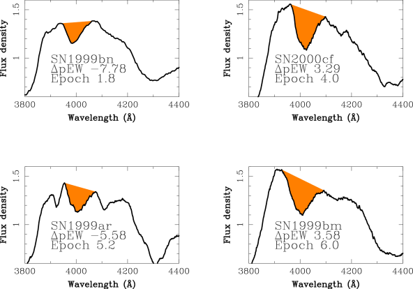
Figure 1.— The Siii $\lambda$4000 feature of SNe Ia. Top left: SN1999bn at day +2 (Siii $\lambda$4000 $\Delta$pEW$=-7.78$ Å). Top right: SN2000cf at day +4 ($\Delta$pEW$=3.29$ Å). Bottom left: SN1999ar at day +5 ($\Delta$pEW$=-5.58$ Å). Bottom right: SN1999bm at day +6 ($\Delta$pEW$=3.58$ Å). Left panels show SNe with narrow Siii $\lambda$4000 feature also after removing epoch dependence, while right panel SNe have wider Si ii $\lambda$ 4000. Stated epochs and $\Delta$pEW measurements are for these individual spectra, and do not correspond to values for SNe with multiple spectra, which is given in Table 2.

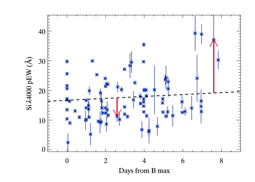
Figure 2.— pEW and $\Delta$pEW measurements of Siii $\lambda$4000. Figure shows measurements of Siii $\lambda$4000 pEW vs. restframe epoch of spectra. The dashed line is the best fit pEW evolution derived using the full sample of N10. $\Delta$pEW is defined as the difference from average evolution for each measurement. Measurements above line will have positive $\Delta$pEW, otherwise negative. Red arrows exemplify one positive and one negative $\Delta$pEW value.

For SNe with multiple spectra in the epoch range, the mean $\Delta$pEW and epoch are used, see Table 2. These steps produce Siii $\lambda$4000 pEW measurements of 55 SNe, 26 from the local sample, 16 from Sloan Digital Sky Survey (SDSS), and 13 from SNLS. The original SDSS and SNLS SN samples are mainly reduced, and in roughly equal fractions, through light curve demands, signal-to-noise requirements, or having no spectra in the studied epoch range.

Of our sample of 55 SNe, 22 objects have three or more spectra in the rest-frame epoch range $-7$ to $+20$ (the range where the Siii $\lambda$6150 velocity typically is well defined). For these SNe we calculate the Siii $\lambda$6150 velocity gradient, a linear fit of velocity decrease per unit time (km s^-1 day^-1). We estimate the uncertainty of these measurements through randomly shifting the velocity measurements (according to errors) and then recalculate the gradient. We use the dispersion among these scrambled gradients to estimate the velocity gradient uncertainty.

See Table 2 for a summary of the data sample.

3. Siii $\lambda$4000 and SALT2 lightcurve color

Figure 3 shows the comparison of Siii $\lambda$4000 $\Delta$pEW measurements for spectra from peak brightness up to +8 days with SALT2 color fits. We find that SNe with smaller pEW widths have bluer light curve colors. This result could be a continuous correlation or signify different subclasses. The Spearman correlation coefficient for the correlation is 0.67, which for the 55 objects corresponds to a rejection of the non-correlation hypothesis at the 5.8$\sigma$ level. If the most reddened SNe are removed ($c>0.3$), the significance changes to 5.2 $\sigma$. Recently, several groups have discussed whether highly reddened objects are affected by an additional, different, source of extinction (Folatelli et al., 2010; Nordin et al., 2011; Foley & Kasen, 2010). The significance of the found correlation was also studied through a simple Monte Carlo test: the pEW values were shuffled so that all color measurements were assigned a random pEW measurement. None of 1000 such iterations yielded a correlation as strong as we find in the data.

Figure 3.— Siii $\lambda$4000 pEW difference ($\Delta$pEW) vs. SALT2 c.

To further understand the Siii $\lambda$4000 region of SNe Ia we have studied how $\Delta$pEW measurements vary with other spectral properties. In Figure 4 we compare Siii $\lambda$4000 $\Delta$pEW measurements of spectra taken at peak brightness up to 8 days past peak, in rest-frame with Siii $\lambda$6150 velocity gradient. There is a strong correlation where SNe with wider Siii $\lambda$4000 features have steeper velocity gradients, thus faster photospheric velocity evolution. The Spearman correlation coefficient for the velocity gradient correlation is $-0.73$, which for the 20 objects corresponds to a rejection of the non-correlation hypothesis at the 3.8$\sigma$ level. Removing SNe with SALT2 $c>0.3$, the significance becomes 4.3 $\sigma$.

Figure 4.— Siii $\lambda$4000 $\Delta$pEW vs. velocity gradient of Siii $\lambda$6150.

3.1. Systematic Effects

Here we investigate if the correlation between Siii $\lambda$4000 width and SALT2 color could be caused by systematic effects connected to our choice of data sets or analysis method. In Figure 5 we show the information from Figure 3 while highlighting the three different samples (local, SDSS, and SNLS). These all have different selection criteria, signal to noise levels, and host subtraction methods. Local SNe have high signal to noise and the host galaxy contamination is, in general, minimal. SDSS and SNLS SNe have lower signal to noise but are obtained through blind searches. SDSS and SNLS are host subtracted using different techniques (as described in Section 2). SNLS measurements show errors before and after the uncertainty from the rescaled SALT2 parameters. None of these subsamples are driving the trends seen. Each sample, if examined individually, exhibits similar behavior, but at lower significances. If systematic effects such as noise, sample selection, or biased host contamination were responsible for the correlation, samples would not be expected to show the same behavior. See Section 6.4 and Appendices A and B in N10 for a full description of our evaluation of these uncertainties for the SDSS SNe.

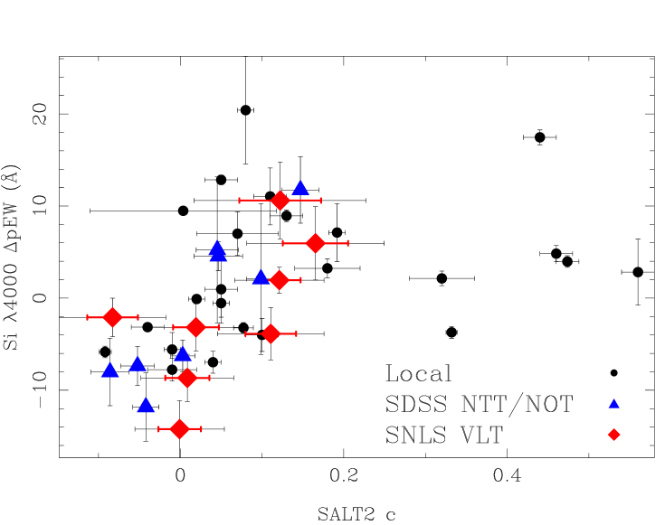
Figure 5.— Siii $\lambda$4000 $\Delta$pEW vs. SALT2 c with the spectral sample origin displayed. The bold, red error bars show the original SNLS light curve errors before the uncertainty from the SALT2 rescaling is applied. Note that SN 1999cl and SN 2003cg, both very highly reddened ($c>1$), were omitted from this figure for clarity.

In a similar way we examine effects from the epoch selection in Figure 6. We find that the correlation cannot be explained by epoch differences. In Table 1 we show how the Spearman Rank Correlation coefficient changes with different epoch and sample cuts. The significance of the correlation, expressed in standard deviations from random scatter, is given in parenthesis. For the Low cont set all SDSS/SNLS SN spectra with estimated host contamination equal to or larger than $20\%$ have been removed. We find that if the epoch range is reduced or the sample restricted the detection $\sigma$ decreases consistently with the reduced number of SNe. We note that both N10 and Blondin et al. (2011) report no strong correlation between Siii $\lambda$4000 width and light curve color for epochs close to peak ($-3$ to $3$ days around peak).

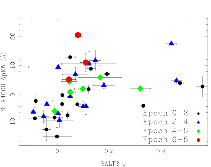
Figure 6.— Siii $\lambda$4000 $\Delta$pEW vs. SALT2 c with epoch information displayed. Note that SN 1999cl and SN 2003cg, both very highly reddened ($c>1$), were omitted from this figure for clarity.

Table 1Spearman Rank Correlation Coefficients

Ep.	All	Local	SDSS	SNLS	Low Cont
0-8	0.67 (5.8)	0.54 (2.9)	0.79 (3.7)	0.51 (1.8)	0.65 (4.9)
0-6	0.70 (5.8)	0.54 (2.7)	0.81 (3.6)	0.62 (2.1)	0.67 (4.8)
3-8	0.71 (4.2)	0.77 (2.7)	0.62 (1.6)	0.50 (1.1)	0.60 (2.5)
3-6	0.84 (4.7)	0.96 (3.8)	0.77 (1.8)	0.60 (1.0)	0.72 (2.7)

In N10 we showed that dust reddening of SN templates has negligible impact on pEWs (See Figure 2 in N10). That study was extended to include combined effects of reddening and noise: we have constructed Monte Carlo tests where randomized reddening and noise are applied to template SN Ia spectra (Hsiao et al., 2007). For extinction, we assume a reddening law as in Cardelli et al. (1989) with $R_{V}=2.1$. The noise is assumed to be Gaussian up to the levels where no measurements can be performed. As with the real sample, we use templates between maximum brightness and 8 days past peak and then subtract the epoch dependence. We find no trend similar to the one observed, for random distributions of $E(B-V)$, noise and spectral epochs.

Since we only investigated the Siii $\lambda$4000 pEW correlation with SALT (in N10) and SALT2 color, we cannot exclude that the effect is related to residual effects from the light curve fitters. Further tests should also include comparisons with other light curve fitters like MLCS2k2 (Jha et al., 2007) or SiFTo (Conley et al., 2008).

Finally, we have investigated whether the measurement pipeline could create a bias: manual measurements were made on the lower signal-to-noise spectra that were rejected during the automatic measurement process. These show an increased scatter, but the trend does not disappear.

In summary, we cannot find any systematic effect that would explain the correlation between Siii $\lambda$4000 pEW and SALT2 color in Figure 3.

4. Discussion

A definitive detection of a correlation between a spectral feature such as Siii $\lambda$4000 and light curve color would imply that at least part of the observed color differences of SNe Ia are intrinsic to the SNe themselves. This intrinsic reddening is connected to the shape and change of the silicon features of SNe Ia. At the same time we expect additional reddening effects, at some level, from (at least) host galaxy dust. With two or more different reddening mechanisms, one of which is intrinsic, it is likely that SN light curve fitters could yield better cosmological constraints if these mechanisms could be taken into account separately.

Besides a possible direct connection to reddening, the results presented here can be studied in the light of recent attempts at finding subtypes of SNe Ia, e.g., the qualitative subtyping scheme introduced by Branch et al. (2006). In Figure 7 we show Siii $\lambda$4000 $\Delta$pEW against SALT2 color, but with the Branch classification (from Branch et al., 2006, 2008) marked. Among the 20 SNe with determined Branch type, all were classified as either CN or BL. There are no Cool or SS SNe, consistent with a sample only consisting of normal SNe Ia. Among the 14 moderately reddened ($c\lesssim 0.3$) SNe with Branch-typing, all SNe with wide Siii $\lambda$4000 ($\Delta$pEW$\gtrsim 3$ Å) are BL SNe, while all with narrow Siii $\lambda$4000 ($\Delta$pEW$\lesssim 3$ Å) are CN. Arsenijevic et al. (2008) found a similar relation between Siii $\lambda$4000 pEW and Branch classification using a wavelet transform technique.

We can further connect Siii $\lambda$4000 measurements (or thereby Branch types) to several recent claims regarding further standardization of SNe: Bailey et al. (2009) and Blondin et al. (2011) use flux ratios, with one “leg” in the $4000$-$4500$ Å region, to standardize low redshift SNe. Wang et al. (2009) use a sample divided according to high or low Siii $\lambda$6150 velocity to obtain either different extinction laws or different intrinsic colors. Foley & Kasen (2010), using the same sample, argue for the later explanation and a connection with the Kasen & Plewa (2007) asymmetric explosion model. In Figure 4 we showed how Siii $\lambda$4000 $\Delta$pEW correlates with Siii $\lambda$6150 velocity gradient. Since Siii $\lambda$6150 velocity and velocity gradient are related (Wang et al., 2009), a connection between Siii $\lambda$4000 width and Siii $\lambda$6150 velocity selected samples is also likely. Our results are thus fully consistent with Wang et al. (2009). Exactly how these spectroscopic properties and subsamples are related, as well as how they are optimally used for SN Ia cosmology, remains to be determined.

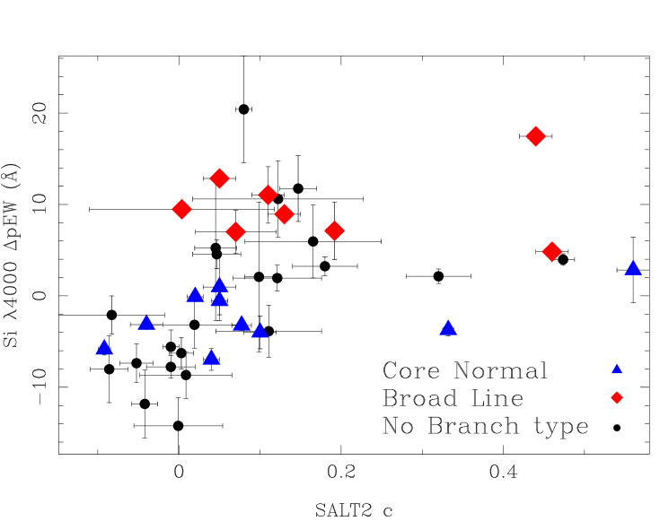
Figure 7.— Siii $\lambda$4000 $\Delta$pEW vs. SALT2 c with the Branch classes marked using different symbols. Note that SN 1999cl and SN 2003cg, both very highly reddened ($c>1$), were omitted from this figure for clarity.

We now ask how Siii $\lambda$4000 $\Delta$pEW measurements relate to SN Ia luminosity. In Figure 8 we compare Siii $\lambda$4000 widths with absolute peak magnitude (rest-frame $B$ band). SNe not in the Hubble flow ($z<0.02$) are not included. We have subtracted the distance modulus, $\mu(z)$, from all magnitudes, assuming a flat $\Lambda$CDM cosmology with $\Omega_{M}=0.27$. We have also corrected the magnitudes for light curve width, $x_{1}$, assuming the $\alpha$ best fit value from Union2 ($\alpha=0.121$).

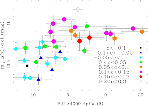
Figure 8.— $\Delta$pEW vs distance and light curve width corrected magnitude. SNe are marked according to SALT2 c (color). Only SNe in the Hubble flow ($z>0.02$) are included.

The data are sparse, but it is possible that two different behaviors exist: SNe with narrow Siii $\lambda$4000 regions exhibit a pEW – magnitude correlation, which could be alternatively described as a reddening – magnitude correlation. SNe with large $\Delta$pEW ($\Delta$pEW$\raise 1.29167pt\hbox{$>$}\kern-7.5pt{\lower 2.79857pt\hbox{$\sim$}}~{}3$ Å) show a small magnitude scatter that is not improved through light curve color corrections.

Guided by the Branch type we now study the effects of dividing the sample at $\sim 3$ Å. For the SNe with $\Delta$pEW$\gtrsim 3$ Å, the magnitude scatter (without any light curve corrections) is 0.15. Fitting a light curve width correction to these SNe reduces the scatter to 0.06. Photometric light curve fitters typically produce magnitude scatters around 0.15 mag after light curve corrections. However, our subset consists of only nine objects, including SNLS SNe up to $z\sim 0.6$. While this result is intriguing, more data are needed for a robust confirmation.

The subsets discussed here could be related to differences between SNe Ia in different host galaxy environments. Recently Sullivan et al. (2010) and Lampeitl et al. (2010) reported that SNe in passive galaxies are intrinsically brighter after light curve corrections. There are also tentative signs that SNe in passive hosts prefer a less steep extinction law. Unfortunately we only have secure host galaxy information for a minority of these SNe, and existing information was obtained using different methods. For low redshift SNe with host galaxy information in the literature we note that three out of 16 SNe with narrow Siii $\lambda$4000 ($\Delta$pEW$<3$ Å) occur in E/S0 galaxies, while none out of 8 SNe with wide Siii $\lambda$4000 ($\Delta$pEW$>3$ Å) occur in E/S0 hosts. For the SDSS sample we found in N10 that hosts of SNe with narrow Siii $\lambda$4000 widths have high specific star formation rate. A coherent analysis of host galaxy properties for our sample is clearly needed. We note that, based on Figure 8, SNe with narrow or wide Siii $\lambda$4000 features would prefer different extinction laws and, possibly, different intrinsic brightness.

The region around 4000 Å is dominated by Siii absorption in normal SNe. However, high signal-to-noise spectra also exhibit smaller absorption features, attributed to Cii, Crii, Coii or Feiii (see, e.g. Garavini et al., 2005; Branch et al., 2008; Scalzo et al., 2010). In spectra with more noise, such small features are not individually resolved. The Siii $\lambda$4000 feature is thus a complex spectral region, where absorption from many different ions might be superimposed. The results presented here need not imply different silicon abundances. Instead, the presence of other elements could cause the measured feature width to change. In N10 we examined composite spectra constructed from SNe with high/low Siii $\lambda$4000 widths. The differences we found could be explained through small additional absorption features. Detailed modeling of this region is needed to fully understand the Siii $\lambda$4000 absorption pattern.

We conclude with two observational remarks. First, the Siii $\lambda$4000 feature is sufficiently blue to be observable in optical bands up to high redshift while the signal-to-noise and resolution requirements for pEW measurements are only moderate (S/N $\sim 12$ in $25$ Å bins, roughly a factor of two less than what flux ratios require). Second, measurements of feature widths do not demand spectrophotometric data, only that the host galaxy contamination is moderate (less than $60$%, see Appendix A in N10). Provided this can be achieved measurements are thus feasible also with multi-fiber observations.

The SNLS spectra already included in this study prove that Siii $\lambda$4000 width measurements on individual high-redshift spectra are possible. For the high redshift ($z\sim 0.5$) SNLS spectra used in this study, observed with VLT FORS1, exposure times of between 40 and 60 minutes were used. Current generation ground-based instruments (e.g., FORS2 or XShooter) are already sensitive enough to make accurate measurements of this spectral indicator out to $z\sim 1$. A future space-based mission (WFIRST) equipped with a slit spectrograph (or IFU) would be able to provide spectral indicator measurements even beyond $z\sim 1$.

If the correlations between light curve color and feature width discussed here can be confirmed this would thus constitute a viable alternative to multi-band photometry (where heavily extincted objects would be removed using the overall spectral shape).

5. Conclusions

We present evidence of a correlation between SALT2 color and Siii $\lambda$4000 pEW of SN Ia spectra observed between $B$-band maximum and $8$ days later. Normal SNe Ia with weak pEW have lower SALT2 $c$ values, while SNe with wide Siii $\lambda$4000 absorptions have higher $c$ (are “redder”). The Spearman correlation coefficient for the correlation is at the $5.8\sigma$ level. We have looked for spurious effects that could produce the observed correlation, but have been unable to identify any.

We can further tie the Siii $\lambda$4000 width to previously defined spectroscopic subclasses: SNe with wide/deep Siii $\lambda$4000 are generally of the “BL” class with large velocity gradients. SNe with narrow Siii $\lambda$4000 are “CN” with small velocity gradients. We also show that for our sample of SNe Ia, distance estimates can be improved using Siii $\lambda$4000 measurements. More data are needed to study any relationship to host galaxy properties and extinction. Siii $\lambda$4000 pEW measurements can, in principle, be done for high redshift SN spectra with reasonable signal-to-noise.

Our understanding of SNe Ia, and their use as standard candles, steadily improves. This process will likely allow us to limit systematic uncertainties and increase the power of SN Ia cosmology.

Table 2 Spectra.

ID	$z$	SALT2 $c$	Siii $\lambda 4000$ $\Delta$pEW (Å)	Siii $\lambda 6150$ Vel. Grad. ($10^{2}$ km s-1 day-1)	Epoch [No. of Spectra]	LC Source	Spectra Source
SN 1989B	0.0024	0.47(0.01)	3.97(0.63)	$-$1.11(0.39)	0[1]	Arsenijevic et al. (2008)	Barbon et al. (1990)
SN 1990N	0.0045	0.08(0.01)	$-$3.23(0.56)	…	1.99[1]	Arsenijevic et al. (2008)	Mazzali et al. (1993); Gómez & López (1998)
SN 1991M	0.0076	0.00(0.11)	9.48(0.11)	…	2.98[1]	Arsenijevic et al. (2008)	Gómez & López (1998)
SN 1996X	0.0078	0.02(0.01)	$-$0.10(0.31)	$-$0.45(0.27)	0.50[2]	Amanullah et al. (2010)	Salvo et al. (2001)
SN 1997do	0.0105	0.11(0.02)	11.04(3.09)	$-$0.8(0.88)	7.84[1]	Amanullah et al. (2010)	Matheson et al. (2008)
SN 1997dt	0.0078	0.56(0.02)	2.82(3.58)	$-$0.82(0.69)	1.12[2]	Amanullah et al. (2010)	Matheson et al. (2008)
SN 1998V	0.0172	0.04(0.01)	$-$6.96(1.19)	$-$0.27(0.35)	1.13[2]	Amanullah et al. (2010)	Matheson et al. (2008)
SN 1998aq	0.0050	$-$0.09(0.01)	$-$5.85(0.62)	$-$0.37(0.24)	3.32[15]	Arsenijevic et al. (2008)	Matheson et al. (2008); Branch et al. (2003)
SN 1998bu	0.0027	0.33(0.01)	$-$3.72(0.64)	…	0.42[1]	Arsenijevic et al. (2008)	Matheson et al. (2008); Jha et al. (1999); Cappellaro et al. (2001); Spyromilio et al. (2004)
SN 1998dh	0.0092	0.13(0.02)	8.93(0.62)	$-$1.05(1.07)	0[1]	Amanullah et al. (2010)	Matheson et al. (2008)
SN 1998dm	0.0065	0.32(0.04)	2.14(0.79)	$-$0.58(0.32)	4.09[1]	Amanullah et al. (2010)	Matheson et al. (2008)
SN 1998eg	0.0235	0.05(0.02)	0.96(3.69)	$-$0.79(0.31)	4.60[2]	Amanullah et al. (2010)	Matheson et al. (2008)
SN 1999ao	0.0544	0.08(0.01)	20.41(5.84)	$-$2.15(0.52)	6.64[1]	Amanullah et al. (2010)	Garavini et al. (2007a)
SN 1999ar	0.1561	$-$0.01(0.01)	$-$5.58(1.84)	…	5.22[1]	Amanullah et al. (2010)	Garavini et al. (2007a)
SN 1999bm	0.1428	0.18(0.04)	3.24(1.03)	…	3.94[2]	Amanullah et al. (2010)	Garavini et al. (2007a)
SN 1999bn	0.1285	$-$0.01(0.03)	$-$7.78(1.24)	…	1.77[1]	Amanullah et al. (2010)	Garavini et al. (2007a)
SN 1999cc	0.0315	0.05(0.02)	12.84(0.52)	$-$1.23(0.25)	1.31[1]	Amanullah et al. (2010)	Matheson et al. (2008)
SN 1999cl	0.0087	1.20(0.01)	13.09(0.72)	$-$2.22(0.4)	0[1]	Amanullah et al. (2010)	Matheson et al. (2008)
SN 1999ej	0.0154	0.07(0.05)	7.00(2.37)	$-$0.88(0.42)	2.53[2]	Amanullah et al. (2010)	Matheson et al. (2008)
SN 1999gd	0.0193	0.46(0.02)	4.83(0.88)	…	2.05[1]	Amanullah et al. (2010)	Matheson et al. (2008)
SN 2000cf	0.0365	0.04(0.02)	1.67(1.83)	$-$0.53(0.44)	3.31[2]	Amanullah et al. (2010)	Matheson et al. (2008)
SN 2000fa	0.0218	0.10(0.02)	$-$4.00(1.80)	$-$0.66(0.33)	2.83[2]	Amanullah et al. (2010)	Matheson et al. (2008)
SN 2002bo	0.0053	0.44(0.02)	17.46(0.80)	$-$1.37(1.27)	3.98[1]	Amanullah et al. (2010)	Benetti et al. (2004)
SN 2002er	0.0086	0.19(0.01)	7.12(3.15)	$-$0.99(0.14)	1.98[3]	Arsenijevic et al. (2008)	Kotak et al. (2005)
SN 2003cg	0.0041	1.16(0.01)	20.01(3.40)	$-$0.54(0.18)	6.97[1]	Amanullah et al. (2010)	Elias-Rosa et al. (2006)
SN 2003du	0.0064	$-$0.04(0.02)	$-$3.15(0.24)	$-$0.13(0.14)	2.98[5]	Amanullah et al. (2010)	Stanishev et al. (2007); Anupama et al. (2005); Gerardy (2005)
SN 2005cf	0.0070	0.05(0.01)	$-$0.55(1.53)	$-$0.73(0.15)	3.77[5]	Amanullah et al. (2010)	Garavini et al. (2007b); Leonard (2007)
SN 2006fx	0.2239	0.11(0.02)	$-$0.99(2.93)	…	3.44[1]	SDSS-II	Östman et al. (2011)
SN 2006kq	0.1985	$-$0.02(0.02)	$-$0.72(2.55)	…	1.78[1]	SDSS-II	Östman et al. (2011)
SN 2006nw	0.1570	0.00(0.01)	$-$6.27(1.73)	…	2.59[1]	SDSS-II	Östman et al. (2011)
SN 2007jd	0.0727	0.23(0.03)	2.84(1.39)	$-$5.6(2.5)	1.16[1]	SDSS-II	Östman et al. (2011)
SN 2007jk	0.1828	0.15(0.02)	11.74(3.61)	…	3.35[1]	SDSS-II	Östman et al. (2011)
SN 2007ka	0.2180	$-$0.05(0.02)	$-$7.37(2.12)	…	2.72[1]	SDSS-II	Östman et al. (2011)
SN 2007lh	0.1980	0.05(0.03)	5.23(7.93)	…	6.74[1]	SDSS-II	Östman et al. (2011)
SN 2007lm	0.2130	0.10(0.02)	2.07(8.19)	…	4.53[1]	SDSS-II	Östman et al. (2011)
SN 2007ol	0.0560	0.05(0.03)	4.55(1.57)	$-$1.38(0.52)	5.24[1]	SDSS-II	Östman et al. (2011)
SN 2007pf	$-$1.000	$-$0.02(0.02)	$-$11.94(1.56)	…	4.24[1]	SDSS-II	Östman et al. (2011)
SN 2007pu	0.0890	$-$0.04(0.02)	$-$11.83(3.71)	…	1.22[1]	SDSS-II	Östman et al. (2011)
SN 2007qg	0.3139	$-$0.02(0.03)	$-$10.31(3.13)	…	4.68[1]	SDSS-II	Östman et al. (2011)
SN 2007qh	0.2477	0.10(0.02)	17.91(8.32)	…	7.60[1]	SDSS-II	Östman et al. (2011)
SN 2007ql	$-$1.000	$-$0.00(0.02)	$-$3.32(2.50)	…	1.12[1]	SDSS-II	Östman et al. (2011)
SN 2007qs	0.2910	$-$0.09(0.02)	$-$8.03(3.65)	…	1.71[1]	SDSS-II	Östman et al. (2011)
SNLS 03D4at	$-$1.000	$-$0.00(0.14)	$-$6.94(3.60)	…	5.48[1]	SDSS-II	Östman et al. (2011)
SNLS 04D1rh	0.4360	$-$0.00(0.05)	$-$14.23(3.11)	…	0.05[1]	Guy et al. (2010)	Balland et al. (2009)
SNLS 04D2fp	0.4150	0.02(0.06)	$-$3.17(2.57)	…	1.81[1]	Guy et al. (2010)	Balland et al. (2009)
SNLS 04D2fs	0.3570	0.12(0.05)	1.94(1.41)	…	1.73[1]	Guy et al. (2010)	Balland et al. (2009)
SNLS 04D2mc	0.3480	0.15(0.07)	$-$4.72(4.05)	…	6.46[1]	SDSS-II	Östman et al. (2011)
SNLS 04D4bq	0.5500	0.17(0.08)	5.95(3.98)	…	5.13[1]	Guy et al. (2010)	Balland et al. (2009)
SNLS 05D1cb	$-$1.000	0.04(0.09)	$-$11.61(4.31)	…	4.25[1]	SDSS-II	Östman et al. (2011)
SNLS 05D2ac	0.4790	0.01(0.06)	$-$8.67(2.56)	…	2.04[1]	Guy et al. (2010)	Balland et al. (2009)
SNLS 05D2dy	0.5100	$-$0.08(0.07)	$-$2.09(2.08)	…	1.11[1]	Guy et al. (2010)	Balland et al. (2009)
SNLS 05D4be	$-$1.000	$-$0.12(0.06)	$-$11.16(2.85)	…	3.88[1]	SDSS-II	Östman et al. (2011)
SNLS 05D4cw	0.3750	$-$0.09(0.05)	$-$4.31(5.68)	…	6.95[1]	SDSS-II	Östman et al. (2011)
SNLS 05D4ek	0.5360	0.11(0.07)	$-$3.87(2.84)	…	2.08[1]	Guy et al. (2010)	Balland et al. (2009)
SNLS 06D2cc	0.5320	0.12(0.11)	10.60(4.17)	…	3.26[1]	Guy et al. (2010)	Balland et al. (2009)

Table 2continued.

References

- Amanullah et al. (2010) Amanullah, R., Lidman, C., Rubin, D., et al. 2010, ApJ, 716, 712
- Anupama et al. (2005) Anupama, G. C., Sahu, D. K., & Jose, J. 2005, A&A, 429, 667
- Arsenijevic et al. (2008) Arsenijevic, V., Fabbro, S., Mourão, A. M., & Rica da Silva, A. J. 2008, A&A, 492, 535
- Bailey et al. (2009) Bailey, S., Aldering, G., Antilogus, P., et al. 2009, ArXiv e-prints 0905.0340
- Balland et al. (2009) Balland, C., Baumont, S., Basa, S., et al. 2009, A&A, 507, 85
- Barbon et al. (1990) Barbon, R., Benetti, S., Rosino, L., Cappellaro, E., & Turatto, M. 1990, A&A, 237, 79
- Baumont et al. (2008) Baumont, S., Balland, C., Astier, P., et al. 2008, A&A, 491, 567
- Benetti et al. (2005) Benetti, S., Cappellaro, E., Mazzali, P. A., et al. 2005, ApJ, 623, 1011
- Benetti et al. (2004) Benetti, S., Meikle, P., Stehle, M., et al. 2004, MNRAS, 348, 261
- Blondin et al. (2011) Blondin, S., Mandel, K. S., & Kirshner, R. P. 2011, A&A, 526, A81+
- Branch et al. (2006) Branch, D., Dang, L. C., Hall, N., et al. 2006, PASP, 118, 560
- Branch et al. (2003) Branch, D., Garnavich, P., Matheson, T., et al. 2003, AJ, 126, 1489
- Branch et al. (2008) Branch, D., Jeffery, D. J., Parrent, J., et al. 2008, PASP, 120, 135
- Bronder et al. (2008) Bronder, T. J., Hook, I. M., Astier, P., et al. 2008, A&A, 477, 717
- Cappellaro et al. (2001) Cappellaro, E., Patat, F., Mazzali, P. A., et al. 2001, ApJ, 549, L215
- Cardelli et al. (1989) Cardelli, J. A., Clayton, G. C., & Mathis, J. S. 1989, ApJ, 345, 245
- Conley et al. (2008) Conley, A., Sullivan, M., Hsiao, E. Y., et al. 2008, ApJ, 681, 482
- Elias-Rosa et al. (2006) Elias-Rosa, N., Benetti, S., Cappellaro, E., et al. 2006, MNRAS, 369, 1880
- Elias-Rosa et al. (2008) Elias-Rosa, N., Benetti, S., Turatto, M., et al. 2008, MNRAS, 384, 107
- Folatelli et al. (2010) Folatelli, G., Phillips, M. M., Burns, C. R., et al. 2010, AJ, 139, 120
- Foley et al. (2008) Foley, R. J., Filippenko, A. V., Aguilera, C., et al. 2008, ApJ, 684, 68
- Foley & Kasen (2010) Foley, R. J. & Kasen, D. 2010, ArXiv e-prints 1011.4517
- Frieman et al. (2008) Frieman, J. A., Bassett, B., Becker, A., et al. 2008, AJ, 135, 338
- Garavini et al. (2005) Garavini, G., Aldering, G., Amadon, A., et al. 2005, AJ, 130, 2278
- Garavini et al. (2007a) Garavini, G., Folatelli, G., Nobili, S., et al. 2007a, A&A, 470, 411
- Garavini et al. (2007b) Garavini, G., Nobili, S., Taubenberger, S., et al. 2007b, A&A, 471, 527
- Gerardy (2005) Gerardy, C. L. 2005, in Astronomical Society of the Pacific Conference Series, Vol. 342, 1604-2004: Supernovae as Cosmological Lighthouses, ed. M. Turatto, S. Benetti, L. Zampieri, & W. Shea, 250–+
- Gómez & López (1998) Gómez, G. & López, R. 1998, AJ, 115, 1096
- Goobar (2008) Goobar, A. 2008, ApJ, 686, L103
- Gunn et al. (1998) Gunn, J. E., Carr, M., Rockosi, C., et al. 1998, AJ, 116, 3040
- Guy et al. (2007) Guy, J., Astier, P., Baumont, S., et al. 2007, A&A, 466, 11
- Guy et al. (2005) Guy, J., Astier, P., Nobili, S., Regnault, N., & Pain, R. 2005, A&A, 443, 781
- Guy et al. (2010) Guy, J., Sullivan, M., Conley, A., et al. 2010, ArXiv e-prints 1010.4743
- Hamuy et al. (1996) Hamuy, M., Phillips, M. M., Suntzeff, N. B., et al. 1996, AJ, 112, 2391
- Holtzman et al. (2008) Holtzman, J. A., Marriner, J., Kessler, R., et al. 2008, AJ, 136, 2306
- Howell et al. (2007) Howell, D. A., Sullivan, M., Conley, A., & Carlberg, R. 2007, ApJ, 667, L37
- Hsiao et al. (2007) Hsiao, E. Y., Conley, A., Howell, D. A., et al. 2007, ApJ, 663, 1187
- Jha et al. (1999) Jha, S., Garnavich, P., Challis, P., Kirshner, R., & Berlind, P. 1999, IAU Circ., 7149, 2
- Jha et al. (2007) Jha, S., Riess, A. G., & Kirshner, R. P. 2007, ApJ, 659, 122
- Kasen & Plewa (2007) Kasen, D. & Plewa, T. 2007, ApJ, 662, 459
- Kelly et al. (2010) Kelly, P. L., Hicken, M., Burke, D. L., Mandel, K. S., & Kirshner, R. P. 2010, ApJ, 715, 743
- Kotak et al. (2005) Kotak, R., Meikle, W. P. S., Pignata, G., et al. 2005, A&A, 436, 1021
- Krisciunas et al. (2007) Krisciunas, K., Garnavich, P. M., Stanishev, V., et al. 2007, AJ, 133, 58
- Krisciunas et al. (2006) Krisciunas, K., Prieto, J. L., Garnavich, P. M., et al. 2006, AJ, 131, 1639
- Lampeitl et al. (2010) Lampeitl, H., Smith, M., Nichol, R. C., et al. 2010, ArXiv e-prints 1005.4687
- Leonard (2007) Leonard, D. C. 2007, in American Institute of Physics Conference Series, Vol. 937, Supernova 1987A: 20 Years After: Supernovae and Gamma-Ray Bursters, ed. S. Immler, K. Weiler, & R. McCray, 311–315
- Li et al. (2010) Li, W., Leaman, J., Chornock, R., et al. 2010, ArXiv e-prints 1006.4612
- Maeda et al. (2010) Maeda, K., Benetti, S., Stritzinger, M., et al. 2010, Nature, 466, 82
- Mannucci et al. (2005) Mannucci, F., Della Valle, M., Panagia, N., et al. 2005, A&A, 433, 807
- Matheson et al. (2008) Matheson, T., Kirshner, R. P., Challis, P., et al. 2008, AJ, 135, 1598
- Maund et al. (2010) Maund, J. R., Hoeflich, P. A., Patat, F., et al. 2010, ArXiv e-prints 1008.0651
- Mazzali et al. (1993) Mazzali, P. A., Lucy, L. B., Danziger, I. J., et al. 1993, A&A, 269, 423
- Nobili & Goobar (2008) Nobili, S. & Goobar, A. 2008, A&A, 487, 19
- Nordin et al. (2008) Nordin, J., Goobar, A., & Jönsson, J. 2008, Journal of Cosmology and Astro-Particle Physics, 2, 8
- Nordin et al. (2011) Nordin, J., Östman, L., Goobar, A., et al. 2011, A&A, 526, A119+
- Östman et al. (2011) Östman, L., Nordin, J., Goobar, A., et al. 2011, A&A, 526, A28+
- Patat et al. (1996) Patat, F., Benetti, S., Cappellaro, E., et al. 1996, MNRAS, 278, 111
- Perlmutter et al. (1999) Perlmutter, S., Aldering, G., Goldhaber, G., et al. 1999, ApJ, 517, 565
- Phillips (1993) Phillips, M. M. 1993, ApJ, 413, L105
- Riess et al. (1998) Riess, A. G., Filippenko, A. V., Challis, P., et al. 1998, AJ, 116, 1009
- Sako et al. (2008) Sako, M., Bassett, B., Becker, A., et al. 2008, AJ, 135, 348
- Salvo et al. (2001) Salvo, M. E., Cappellaro, E., Mazzali, P. A., et al. 2001, MNRAS, 321, 254
- Scalzo et al. (2010) Scalzo, R. A., Aldering, G., Antilogus, P., et al. 2010, ApJ, 713, 1073
- Scannapieco & Bildsten (2005) Scannapieco, E. & Bildsten, L. 2005, ApJ, 629, L85
- Spyromilio et al. (2004) Spyromilio, J., Gilmozzi, R., Sollerman, J., et al. 2004, A&A, 426, 547
- Stanishev et al. (2007) Stanishev, V., Goobar, A., Benetti, S., et al. 2007, A&A, 469, 645
- Sullivan et al. (2010) Sullivan, M., Conley, A., Howell, D. A., et al. 2010, ArXiv e-prints 1003.5119
- Sullivan et al. (2009) Sullivan, M., Ellis, R. S., Howell, D. A., et al. 2009, ApJ, 693, L76
- Tripp (1998) Tripp, R. 1998, A&A, 331, 815
- Walker et al. (2011) Walker, E. S., Hook, I. M., Sullivan, M., et al. 2011, MNRAS, 410, 1262
- Wang et al. (2009) Wang, X., Filippenko, A. V., Ganeshalingam, M., et al. 2009, ApJ, 699, L139
- Wang et al. (2008) Wang, X., Li, W., Filippenko, A. V., et al. 2008, ApJ, 675, 626
- York et al. (2000) York, D. G., Adelman, J., Anderson, Jr., J. E., et al. 2000, AJ, 120, 1579