The plasma emission model of RBS1774

In the present paper we construct a self-consistent theory, interpreting the observational properties of RBS1774. It is well known that the distribution function of relativistic particles is one-dimensional at the pulsar surface. However, cyclotron instability causes an appearance of transverse momenta of relativistic electrons, which as a result, start to radiate in the synchrotron regime. We study the process of the quasi-linear diffusion developed by means of the cyclotron instability on the basis of the Vlasov’s kinetic equation. This mechanism provides generation of measured optical and X-ray emission on the light cylinder lengthscales. A different approach of the synchrotron theory is considered, giving the spectral energy distribution that is in a good agreement with the XMM-Newton observational data. We also provide the possible explanation of the spectral feature at $0.7$keV, in the framework of the model.

1 Introduction

RBS1774 (1RXS J214303.7+065419) has been the most recent XDIN (X ray dim isolated neutron star) to be found (Zampieri et al., 2001). Its X-ray spectrum is well reproduced by an absorbed blackbody with a temperature $kT\sim 100$eV and with a total column density of $n_{H}\sim 3\cdot 10^{20}cm^{-2}$. Application of more sophisticated, and physically motivated models for the surface emission (atmospheric models) result in worse agreement with the data (Zane et al., 2005). According to Schwope et al. (2009), a fit to the X-ray spectra extracted from RGS spectrographs onboard XMM-Newton yields that the best result is obtained when the two-temperature blackbody model is used. But the same model applied to the X-ray spectra extracted from three EPIC detectors does not improve the fit compared to the simple blackbody model. However, the formation of a non-uniform distribution of the surface temperature is more likely artificial and needs to be examined by convincing theory.

Alternatively, the observational properties of RBS1774 can be explained in the framework of the plasma emission model first developed by Machabeli & Usov (1979) and Lominadze et al. (1983). According to these works, in the electron-positron plasma of a pulsar magnetosphere the waves excited by the cyclotron resonance interact with particles, leading to the appearance of pitch angles, which obviously causes synchrotron radiation. We suppose that the X-ray emission from this object is generated by the synchrotron mechanism. According to the standard theory of the synchrotron emission (Bekefi & Barrett, 1977; Ginzburg, 1981) the typical synchrotron spectrum is a power-law, when the present model suggests different spectral distribution. The main reason for this is that we take into account the mechanism of creation of the pitch angles, consequently restricting their values. Contrary to this, in the standard theory of the synchrotron radiation, it is assumed that along the line of sight the magnetic field is chaotic, leading to the broad interval (from $0$ to $\pi$) of the pitch angles. The present model gives successful fit for the observed X-ray spectrum, when the originally excited cyclotron modes enter the same domain as the measured optical emission of RBS1774. We suppose that the observed spectral feature at $0.7$keV in the X-ray spectrum of RBS1774 is caused by wave damping process developed near the light cylinder due to the cyclotron instability.

In this paper, we describe the emission model (Sec. 2), derive theoretical X-ray spectrum of RBS1774 and fit with XMM-Newton observations (Sec. 3), explain the possible nature of the observed spectral feature at $\sim 0.7$keV (Sec.4), and discuss our results (Sec. 5).

2 Emission model

The distribution function of relativistic particles is one dimensional at the pulsar surface, because any transverse momenta ($p_{\perp}$) of relativistic electrons are lost in a very short time($\leq 10^{-20}$s) via synchrotron emission in very strong magnetic fields. For typical pulsars the plasma consists of the following components: the bulk of plasma with an average Lorentz-factor $\gamma_{p}\simeq 10^{2}$, a tail on the distribution function with $\gamma_{t}\simeq 10^{5}$, and the primary beam with $\gamma_{b}\simeq 10^{7}$ (see Fig. 1). However, plasma with an anisotropic distribution function becomes unstable, which can lead to a wave excitation in the pulsar magnetosphere. The generation of waves is possible during the further motion of the relativistic particles along the dipolar magnetic field lines if the condition of cyclotron resonance is fulfilled (Kazbegi et al., 1991):

$$\omega-k_{{}_{\|}}V_{{}_{\|}}-k_{x}u_{x}+\frac{\omega_{B}}{\gamma_{r}}=0,$$ (1)

where $u_{x}=cV_{\varphi}\gamma_{r}/\rho\omega_{B}$ is the drift velocity of the particles due to curvature of the field lines, $\rho$ is the radius of curvature of the field lines and $\omega_{B}=eB/mc$ is the cyclotron frequency. During the generation of waves by resonant particles, one also has a simultaneous feedback of these waves on the electrons (Vedenov et al., 1961). This mechanism is described by quasi-linear diffusion, leading to the diffusion of particles as along as across the magnetic field lines. Therefore, resonant electrons acquire transverse momenta (pitch angles) and, as a result, start to radiate through the synchrotron mechanism.

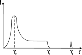
Figure 1: Distribution function of a one-dimensional plasma in the pulsar magnetosphere. Left corresponds to secondary particles, right to the primary beam.

The kinetic equation for the distribution function of the resonant particles can be written as (Machabeli & Usov, 1979; Machabeli et al., 2002):

$$\frac{\partial\textit{f }^{0}}{\partial t}+\frac{\partial}{\partial p_{\parallel}}\left\{(G_{\parallel}+F_{\parallel}+Q_{\parallel})\textit{f }^{0}\right\}+\frac{1}{p_{\perp}}\frac{\partial}{\partial p_{\perp}}\left\{p_{\perp}(G_{\perp}+F_{\perp})\textit{f }^{0}\right\}=$$

$$=\frac{1}{p_{\perp}}\frac{\partial}{\partial p_{\perp}}\left\{p_{\perp}\left(D_{\perp,\perp}\frac{\partial}{\partial p_{\perp}}+D_{\perp,\parallel}\frac{\partial}{\partial p_{\parallel}}\right)\textit{f }^{0}\left(\mathbf{p}\right)\right\}+$$

$$+\frac{\partial}{\partial p_{\parallel}}\left\{\left(D_{\parallel,\perp}\frac{\partial}{\partial p_{\perp}}+D_{\parallel,\parallel}\frac{\partial}{\partial p_{\parallel}}\right)\textit{f }^{0}\left(\mathbf{p}\right)\right\}.$$ (2)

where $G$ is the force responsible for conserving the adiabatic invariant $p_{\perp}^{2}/B(r)=$const, $F$- is the radiation deceleration force produced by synchrotron emission, and $Q_{\parallel}$ is the reaction force of the curvature radiation. They can be written in the form:

$$G_{\perp}=-\frac{mc^{2}}{\rho}\gamma_{r}\psi,\qquad\qquad G_{\parallel}=\frac{mc^{2}}{\rho}\gamma_{r}\psi^{2},$$ (3)

$$F_{\perp}=-\alpha_{s}\psi\left(1+\gamma_{r}^{2}\psi^{2}\right),\qquad F_{\parallel}=-\alpha_{s}\gamma_{r}^{2}\psi^{2},$$ (4)

$$Q_{\parallel}=-\alpha_{c}\gamma_{r}^{4},$$ (5)

where $\alpha_{s}=2e^{2}\omega_{B}^{2}/3c^{2}$, $\alpha_{c}=2e^{2}/3\rho^{2}$ and $\psi\approx p_{\perp}/p_{\parallel}\ll 1$ is the pitch angle.

Now let us compare the transverse components of the forces $G$ and $F$. If we consider the case $\gamma\psi\gg 1$ we will have :

$$\frac{G_{\perp}}{F_{\perp}}=\frac{3m^{3}c^{6}}{2e^{4}B_{s}^{2}}\frac{\gamma}{\rho}\left(\frac{r}{R_{s}}\right)^{6}\frac{1}{\gamma^{2}\psi^{2}}.$$ (6)

where $B_{s}$ is the magnetic field at the star surface, $R_{s}$ is the star radius and $r$ is the distance from the pulsar. For the typical parameter values of pulsars $|G_{\perp}|\ll|F_{\perp}|$. Then taking into account that $\partial/\partial\psi\gg\partial/\partial\gamma$ the equation for the diffusion across the magnetic field can be written in the form (Chkheidze et al., 2010)

$$\frac{\partial\textit{f }^{0}}{\partial t}+\frac{1}{p_{\perp}}\frac{\partial}{\partial p_{\perp}}\left(p_{\perp}F_{\perp}\textit{f }^{0}\right)=\frac{1}{p_{\perp}}\frac{\partial}{\partial p_{\perp}}\left(p_{\perp}D_{\perp,\perp}\frac{\partial\textit{f }^{0}}{\partial p_{\perp}}\right).$$ (7)

where

$$D_{\perp,\perp}=\frac{e^{2}}{8c}\delta|E_{k}|^{2}$$ (8)

is the diffusion coefficient and $|E_{k}|^{2}$ is the density of electric energy in the waves.

The transversal quasi-linear diffusion increases the pitch-angle, whereas force F resists this process, leading to the stationary state ($\partial\textit{f}/\partial t=0$). Then the solution of Eq. (7) is

$$\textit{f}_{\perp}=Cexp\left(\int\frac{F_{\perp}}{D_{\perp,\perp}}dp_{\perp}\right)=Ce^{-\left(\frac{p_{\perp}}{p_{\perp_{0}}}\right)^{4}}.$$ (9)

To evaluate $p_{\perp_{0}}$, we use the quantity

$$|E_{k}|^{2}\approx\frac{1}{2}\frac{mc^{2}n_{b}\gamma_{b}c}{\omega},$$ (10)

where $\omega$ is the frequency of original waves, excited during the cyclotron resonance and can be estimated from Eq. (1) as follows $\omega\approx\omega_{B}/\delta\gamma_{r}$. Consequently, we will get

$$p_{\perp_{0}}\approx\frac{\pi^{1/2}}{B\gamma_{p}^{2}}\left(\frac{3m^{9}c^{11}\gamma_{b}^{5}}{32e^{6}P^{3}}\right)^{1/4}.$$ (11)

The mean value of the pitch-angle $\psi_{0}\approx p_{\perp_{0}}/p_{\parallel}\simeq 10^{-3}$ (i. e. the assumption $\gamma_{r}\psi_{0}\gg 1$ done at the beginning of our computations proves to be true). As a result of the appearance of the pitch angles, the synchrotron emission is generated.

3 X-ray spectrum

Let us consider the synchrotron emission of the set of electrons. The number of emitting particles in the elementary $dV$ volume is $p_{\perp}\textit{f }dp_{\perp}dp_{\parallel}dVd\Omega_{\tau}$, with momenta from the intervals $[p_{\perp},p_{\perp}+dp_{\perp}]$ and $[p_{\parallel},p_{\parallel}+dp_{\parallel}]$, and with the velocities that lie inside the solid angle $d\Omega_{\tau}$ near the direction of $\@vec{\tau}$. If we write the parallel distribution function of the emitting particles as $\int p_{\perp}\textit{f}dp_{\perp}\equiv\textit{f}_{\parallel}(p_{\parallel})$, then the emission flux of the set of electrons will be (Ginzburg, 1981)

$$F_{\epsilon}=\int I_{e}\textit{f}_{\parallel}(p_{\parallel})dp_{\parallel}dVd\Omega_{\tau},$$ (12)

where $I_{e}$ is the Stokes parameter, which is additive in this case, as the observed synchrotron radiation wavelength $\lambda$ is much less than the value of $n^{-1/3}$ - the average distance between particles, where $n$ is the density of plasma component electrons. The integral (12) is easily reduced to (see Ginzburg (1981))

$$F_{\epsilon}\propto\int\textit{f}_{\parallel}(p_{\parallel})B\psi\frac{\epsilon}{\epsilon_{m}}\left[\int_{\epsilon/\epsilon_{m}}^{\infty}K_{5/3}(z)dz\right]dp_{\parallel}.$$ (13)

Here $\epsilon_{m}\approx 5\cdot 10^{-12}B\psi\gamma^{2}$keV is the photon energy of the maximum of synchrotron spectrum of a single electron and $K_{5/3}(z)$ is a Macdonald function. After substituting the mean value of the pitch-angle in the above expression for $\epsilon_{m}$, we get

$$\epsilon_{m}\simeq 5\cdot 10^{-12}\frac{\pi^{1/2}}{\gamma_{p}^{2}}\left(\frac{3m^{5}c^{7}\gamma_{b}^{9}}{32e^{6}P^{3}}\right)^{1/4}$$ (14)

For the primary beam electrons with the Lorentz factor $\gamma_{b}\sim 10^{7}$ the emitted photon energy $\epsilon_{m}\sim 0.1$keV comes in the energy domain of the observed X-ray emission of RBS1774. Thus we suppose that the measured X-ray spectrum is the result of the synchrotron emission of primary beam electrons (the resonance occurs on the right slope of the distribution function of beam electrons (see Fig. 1)), switched on as the result of acquirement of pitch angles by particles during the quasi-linear stage of the cyclotron instability.

To find the synchrotron flux in our case, we need to know the one-dimensional distribution function of the emitting particles $\textit{f}_{\parallel}$. Let us multiply both sides of Eq. (2) on $p_{\perp}$ and integrate it over $p_{\perp}$. Using Eqs. (3), (4), (5) and the following expressions for the diffusion coefficients (Chkheidze et al., 2010)

$$D_{\perp,\parallel}=D_{\parallel\perp}=-\frac{e^{2}}{8c}\psi|E_{k}|^{2},$$ (15)

$$D_{\parallel,\parallel}=\frac{e^{2}}{8c}\psi^{2}\frac{1}{\delta}|E_{k}|^{2}.$$

And also taking into account that the distribution function vanishes at the boundaries of integration, Eq. (2) reduces to

$$\frac{\partial\textit{f}_{\parallel}}{\partial t}=\frac{\partial}{\partial p_{\parallel}}\left[\left({\frac{\alpha_{s}}{m^{2}c^{2}\pi^{1/2}}p_{\perp_{0}}^{2}}+\alpha_{c}\gamma^{4}-\frac{e^{2}}{4mc^{2}\gamma}|E_{k}|^{2}\right)\textit{f}_{\parallel}\right].$$ (16)

Let us estimate the contribution of different terms on the righthand side of Eq. (16). The estimations show that the first term is much bigger than two other terms. Consequently, for the primary-beam electrons instead of Eq. (16), one gets

$$\frac{\partial\textit{f}_{\parallel}}{\partial t}=\frac{\partial}{\partial p_{\parallel}}\left({\frac{\alpha_{s}}{m^{2}c^{2}\pi^{1/2}}p_{\perp_{0}}^{2}\textit{f}_{\parallel}}\right).$$ (17)

Considering the quasi-stationary case we find

$$\textit{f}_{\parallel}\propto\frac{1}{p_{\parallel}^{1/2}|E_{k}|}.$$ (18)

For $\gamma\psi\ll 10^{10}$, a magnetic field inhomogeneity does not affect the process of wave excitation. The equation that describes the cyclotron noise level, in this case, has the form (Lominadze et al., 1983)

$$\frac{\partial|E_{k}|^{2}}{\partial t}=2\Gamma_{c}|E_{k}|^{2}\textit{f}_{\parallel},$$ (19)

where

$$\Gamma_{c}=\frac{\pi^{2}e^{2}}{k_{\parallel}}\textit{f}_{\parallel}(p_{res}),$$ (20)

is the growth rate of the instability. Here $k_{\parallel}$ can be found from the resonance condition (1)

$$k_{\parallel_{res}}\approx\frac{\omega_{B}}{c\delta\gamma_{res}}.$$ (21)

Combining Eqs. (17) and (19) one finds

$$\frac{\partial}{\partial t}\left\{\textit{f}_{\parallel}-\alpha\frac{\partial}{\partial p_{\parallel}}\left(\frac{|E_{k}|}{p_{\parallel}^{1/2}}\right)\right\}=0,$$ (22)

$$\alpha=\left(\frac{4}{3}\frac{e^{2}}{\pi^{5}c^{5}}\frac{\omega_{B}^{6}\gamma_{p}^{3}}{\omega_{p}^{2}}\right)^{1/4},$$ (23)

which reduces to

$$\left\{\textit{f}_{\parallel}-\alpha\frac{\partial}{\partial p_{\parallel}}\left(\frac{|E_{k}|}{p_{\parallel}^{1/2}}\right)\right\}=const.$$ (24)

Taking into account that for the initial moment the major contribution of the lefthand side of the Eq. (24) comes from $\textit{f}_{\parallel_{0}}$, the corresponding expression writes as

$$\textit{f}_{\parallel}-\alpha\frac{\partial}{\partial p_{\parallel}}\left(\frac{|E_{k}|}{p_{\parallel}^{1/2}}\right)=\textit{f}_{\parallel_{0}}.$$ (25)

The distribution function f is proportional to $n\sim 1/r^{3}$, then one should neglect $\textit{f}_{\parallel}$ in comparison with $\textit{f}_{\parallel_{0}}$. Consequently, the above equation reduces to

$$\alpha\frac{\partial}{\partial p_{\parallel}}\left(\frac{|E_{k}|}{p_{\parallel}^{1/2}}\right)+\textit{f}_{\parallel_{0}}=0.$$ (26)

As we can see the function $E_{k}(p_{\parallel})$ drastically depends on the form of the initial distribution of the primary beam electrons. Here we assume that the initial energy distribution in the beam has a Gaussian shape

$$\textit{f}_{b_{0}}=\frac{n_{b}}{\sqrt{\pi}\gamma_{T}}\textrm{ exp}\left[-\frac{\left(\gamma-\gamma_{b}\right)^{2}}{\gamma_{T}^{2}}\right],$$ (27)

where $\gamma_{T}\simeq 10$ - is the half width of the distribution function and $n_{b}=B/Pce$ is the density of primary beam electrons, equal to the Goldreich-Julian density (Goldreich & Julian, 1969). Since $\gamma_{T}\ll\gamma_{b}$, this distribution is very close to $\delta$-function. Consequently, the electron distribution can be taken as monoenergetic.

In this case for the energy density of the waves we get

$$|E_{k}|^{2}\propto p_{\parallel}.$$ (28)

The effective value of the pitch angle depends on $|E_{k}|^{2}$ as follows

$$\psi_{0}=\frac{1}{2\omega_{B}}\left(\frac{3m^{2}c^{3}}{p_{\parallel}^{3}}\frac{\omega_{p}^{2}}{\gamma_{p}^{3}}|E_{k}|^{2}\right)^{1/4}.$$ (29)

According to our emission model, the observed radiation comes from a region near the light cylinder radius, where the magnetic field lines are practically straight and parallel to each other (Osmanov et al., 2009), therefore, electrons with $\psi\approx\psi_{0}$ efficiently emit in the observer’s direction.

Using expression (18), (28) and (29), and replacing the integration variable $p_{\parallel}$ by $x=\epsilon/\epsilon_{m}$, from Eq. (13) we will get

$$F_{\epsilon}\propto\epsilon^{-0.3}\int x^{0.3}\left[\int_{x}^{\infty}K_{5/3}(z)dz\right]dx.$$ (30)

The energy of the beam electrons vary in a small interval. In this case the integral (30) can be approximately expressed by the following function

$$F_{\epsilon}\propto\epsilon^{0.3}exp(-\epsilon/\epsilon_{m}).$$ (31)

We performed a spectral analysis by fitting the model spectrum (Eq. (31)) absorbed by cold interstellar matter, with the combined data extracted of the three EPIC X-ray cameras of the XMM-Newton Telescope. The resulting $\chi^{2}=1.63$ and the amount of interstellar matter $n_{H}=(3.36\pm 0.2)\times 10^{20}cm^{-2}$, which appears to be close to the total Galactic absorption in the source direction ($n_{H}=5\cdot 10^{20}cm^{-2}$ Dickey & Lockman (1990)). The spectral feature at $\sim 0.7$keV that is mostly described as an absorption edge or line (Zane et al., 2005; Schwope et al., 2009) is also evident in our case from inspection of Fig. 2. We find that adding an absorption edge at $0.7$keV improves the fit, leading to a reduced $\chi^{2}=1.50$. The best-fitting energy of the edge is $E_{edge}=0.679$keV, and the optical depth is $\tau_{edge}=0.20$ (see Fig. 3). The fitting results are listed in Table 1. We suppose that existence of the absorption feature in spectra of RBS1774 is caused by wave damping at photon energies $\sim 0.7$keV, which takes place near the light cylinder.

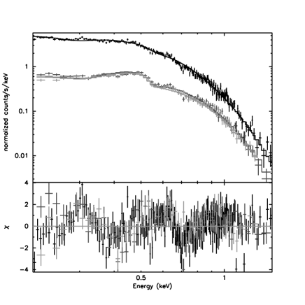
Figure 2: EPIC-pn and EPIC-MOS spectra of RBS1774, fitted with a model.

4 Possible nature of the spectral feature

During the farther motion in the pulsar magnetosphere, the X-ray emission of RBS1774 that is generated on the light cylinder lengthscales, might come in the cyclotron damping range (Khechinashvili & Melikidze, 1997):

$$\omega-k_{{}_{\|}}V_{{}_{\|}}-k_{x}u_{x}-\frac{\omega_{B}}{\gamma_{r}}=0.$$ (32)

The condition for the development of the cyclotron instability may be easily derived for the small angles of propagation with respect to the magnetic field. Representing the dispersion of the waves as

$$\omega=kc,$$ (33)

and neglecting the drift term, the resonance condition (32) may then be written as

$$\frac{1}{2\gamma_{r}^{2}}+\frac{\theta^{2}}{2}=\frac{\omega_{B}}{\omega\gamma_{r}},$$ (34)

where $\theta\approx\psi$ is the angle between the wave vector and the magnetic field. Taking into account that $\psi_{0}^{2}\gg 1/2\gamma_{b}^{2}$ one finds from Eq. (34) the frequency of damped waves

$$\omega_{0}=\frac{2\omega_{B}}{\gamma_{r}\psi^{2}}.$$ (35)

If we assume that the resonant particles are the primary beam electrons, then the estimation shows that on the light cylinder lengthscales $\epsilon_{0}=(h/2\pi)\omega_{0}\simeq 0.7$keV.

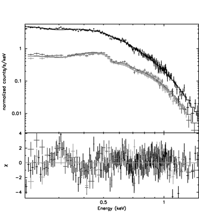
Figure 3: EPIC-pn and EPIC-MOS spectra of RBS1774 fitted with a model, including an absorption edge at $\sim 0.7$keV.

Table 1: The model parameters of RBS1774 for combined fits to EPIC-pn and EPIC-MOS in the energy interval $0.2-1.5$ keV(The fitting results with a pure blackbody model absorbed by cold interstellar matter are from Schwope et al. (2009))

Model	$n_{H}$	$\epsilon_{m}^{-1}$	$kT_{bb}^{\infty}$	$E_{edge/line}$	$\sigma_{line}$	$\tau_{edge/line}$	$\chi^{2}$(dof)
	$(10^{20}cm^{-2})$	(eV)	(eV)	(eV)	(eV)
plasma	$3.36^{+0.20}_{-0.20}$	$7.0\pm 0.2$					$1.63(311)$
plasma*edge	$3.30^{+0.12}_{-0.12}$	$6.9\pm 0.1$		$679^{+13}_{-13}$		$0.20^{+0.03}_{-0.03}$	$1.50(309)$
bbody	$1.85^{+0.17}_{-0.17}$		$103.5\pm 0.8$				$1.81(311)$
bbody*gabs	$1.84^{+0.20}_{-0.17}$		$105.1\pm 0.9$	$731^{+8}_{-13}$	$27^{+16}_{-4}$	$6.5^{+1.2}_{-1.0}$	$1.50(308)$

5 Discussion

According to the generally accepted point of view, the X-ray spectrum of RBS1774 is purely thermal and is best represented by a Planckian shape. A fit with a pure blackbody component absorbed by cold interstellar matter gives $\chi^{2}=1.81$ (Schwope et al., 2009). Including a Gaussian absorption line at $\sim 0.7$keV (as the largest discrepansies between model and data are around $0.7$keV) improves the fit $\chi^{2}=1.50$ (parameters are listed in Tab.1). However, the nature of this spectral feature is not fully clarified as yet. The most likely interpretation is that it is due to proton cyclotron resonance, which implies ultrastrong magnetic field of $B_{cyc}\sim 10^{14}$G (Zane et al., 2005; Rea et al., 2007). Although, the required strong magnetic field is inconstistent with timing measurements giving $B_{dip}=3.2\cdot 10^{19}\sqrt{P\dot{P}}\simeq 2\cdot 10^{13}$G (Kaplan & van Kerkwijk, 2009).

We are not about to reject the existing thermal emission models, but in present paper we propose an alternative explanation of the observed X-ray spectrum of RBS1774. It is supposed that the emission of this source is generated by the synchrotron mechanism. The distribution function of relativistic particles is one dimensional at the pulsar surface, but plasma with an anisotropic distribution function is unstable which can lead to wave excitation. The main mechanism of wave generation in plasmas of the pulsar magnetosphere is the cyclotron instability, which develops on the light cylinder lengthscales. During the quasi-linear stage of the instability, a diffusion of particles arises along and across the magnetic field lines. Therefore, plasma particles acquire transverse momenta and, as a result, the synchrotron mechanism is switched on. If the resonant particles are the primary beam electrons with $\gamma_{b}\simeq 10^{7}$ their synchrotron emission enter the same energy domain as the measured X-ray spectrum of RBS1774.

We construct a self-consistent theory interpreting the observations of RBS1774. Differently from the standard theory of the synchrotron emission (Ginzburg, 1981), which only provides a power-law spectrum with the spectral index less than 1, our approach gives the possibility to obtain different spectral energy distributions. In the standard theory of the synchrotron emission, it is supposed that the observed radiation is collected from a large spacial region in various parts of which, the magnetic field is oriented randomly. Thus, it is supposed that along the line of sight the magnetic field directions are chaotic and when finding emission flux, Eq. (13) is averaged over all directions of the magnetic field (which means integration over $\psi$ varying from $0$ to $\pi$). In our case the emission comes from a region of the pulsar magnetosphere where the magnetic field lines are practically straight and parallel to each other. And differently from standard theory, we take into account the mechanism of creation of the pitch angles. Thus we obtain a certain distribution function of the emitting particles from their perpendicular momenta (see Eq. (10)), which restricts the possible values of the pitch angles. In the framework of the model we obtain the following theoretical X-ray spectrum of RBS1774 $F_{\epsilon}\propto\epsilon^{0.3}exp(-\epsilon/\epsilon_{m})$ and perform a spectral analysis by fitting data from the three EPIC detectors simultaneously. The fit with a model spectrum absorbed by cold interstellar matter yields $\chi^{2}=1.63$ (see parameters in Tab.1).

During the farther motion in the pulsar magnetosphere, the X-ray emission of RBS1774 comes in the cyclotron damping range (see Eq. (32)). If we assume that damping happens on the left slope of the distribution function of primary beam electrons (see Fig. 1), then the photon energy of damped waves will be $\epsilon_{0}=(h/2\pi)\omega_{0}=(h/2\pi)2\omega_{B}/\gamma_{b}\psi^{2}\simeq 0.7$keV. Taking into account the shape of the distribution function of beam electrons, we interpret the large residuals around $\sim 0.7$keV (see Fig. 2) as an absorption edge. Including an absorption edge improves the fit leading to a reduced $\chi^{2}=1.50$. The best-fitting energy of the edge is $E_{edge}=0.679$keV, and the optical depth is $\tau_{edge}=0.20$ (see Tab.1). However, adding an absorption edge to the model spectrum does not produce a statistically significant improvement of the fitting. According to Schwope et al. (2009) if one uses the RGS X-ray spectra of RBS1774 in place of EPIC spectra, the resulting $\chi^{2}$ is changed just marginally when a Gaussian absorption line is included at $\sim 0.7$keV. Thus, we conclude that the nature of the feature at $0.7$keV is uncertain and might be related to calibration uncertainties of the CCDs and the RGS at those very soft X-ray energies. The same can be told about a feature at $\sim 0.3$keV (the large residuals around $0.3$keV are evident from inspection of Fig. 2 and  3). A feature of possible similar nature was detected in EPIC-pn spectra of the much brighter prototypical object RXJ1856.4-3754 and classified as remaining calibration problem by Haberl (2007). Consequently, more data are necessary to finally prove or disprove the existence of those features.

The frequency of the original waves, excited during the cyclotron resonance can be estimated from Eq. (1) as follows $\nu\approx 2\pi\omega_{B}/\delta\gamma_{b}\sim 10^{14}$Hz. As we can see the frequency of cyclotron modes comes in the same domain as the measured optical emission of RBS1774 (Zane et al., 2008; Schwope et al., 2009).

References

- Arons (1981) Arons, J. 1981, In: Proc. Varenna Summer School and Workshop on Plasma Astrophysics, ESA, p.273
- Bekefi & Barrett (1977) Bekefi George & Barrett Alan H., 1977, Electromagnetic vibrations, waves and radiation, The MIT Press, Cambridge, Massachusetts and London, England
- Burwitz et al. (2001) Burwitz, V., Zavlin, V. E., Neuhäuser, R., Predehl, P., Trümper, J. Brinkman, A. C., 2001, A&A, 379, L35
- Burwitz et al. (2003) Burwitz, V., Haberl, F. Neuhäuser, R., Predehl, P., Trümper, J. Zavlin, V. E., 2003, A&A, 399, 1109
- Chkheidze & Machabeli (2007) Chkheidze, N., Machabeli, G., 2007, A&A, 471, 599
- Chkheidze & Lomiashvili (2008) Chkheidze, N., Lomiashvili, D., 2008, NewA, 13, 12
- Chkheidze et al. (2010) Chkheidze, N., Machabeli, G., Osmanov, Z., 2010, ApJ, (submitted)
- Dickey & Lockman (1990) Dickey, J., & Lockman, F. 1990, ARA&A, 28, 215
- Drake et al. (2002) Drake, J. J., Marshall, H. L., Dreizler, S., Freeman, P. E., Fruscione, A., et al. 2002, ApJ, 572, 996
- Ginzburg (1981) Ginzburg, V. L., ”Teoreticheskaia Fizika i Astrofizika” ,Nauka, Moskva 1981
- Goldreich & Julian (1969) Goldreich, P., Julian, W. H., 1969, ApJ, 157, 869
- Haberl (2007) Haberl, F., 2007, Ap&SS, 308, 181
- Ho et al. (2007) Ho, W. C. G., Kaplan, D. L., Chang, P., Adelsberg, M., Potekhin, A. Y., 2007, MNRAS 375, 281H
- Ho (2007) Ho, W. C. G., 2007, MNRAS 380, 71H
- Kaplan & van Kerkwijk (2009) Kaplan, D. L., van Kerkwijk, M. H., 2009, ApJ, 692, 62
- Kazbegi et al. (1991) Kazbegi A. Z., Machabeli G. Z., Melikidze G. I., 1991, MNRAS, 253, 377
- Kazbegi et al. (1996) Kazbegi A. Z., Machabeli G. Z., Melikidze G. I., Shukre C., 1996, A&A, 309, 515
- Khechinashvili & Melikidze (1997) Khechinashvili, D. G., Melikidze, G. I., 1997, A&A, 320, L45
- Lai & Salpeter (1997) Lai, D., Salpeter, E. E., 1997, ApJ, 491, 270
- Lai (2001) Lai, D., 2001, Rev. of Mod. Phys. 73, 629
- Lomiashvili et al. (2006) Lomiashvili D., Machabeli G., & Malov I., 2006, ApJ, 637, 1010
- Lominadze et al. (1983) Lominadze J.G., Machabeli G. Z., & Usov V. V., 1983, Ap&SS, 90, 19L
- Machabeli & Usov (1979) Machabeli, G. Z., & Usov, V. V., 1979 AZh Pi’sma, 5, 445
- Machabeli et al. (2002) Machabeli, G. Z., Luo, Q., Vladimirov, S. V., & Melrose, D. B., 2002, Phys. Rev. E, 65, 036408
- Malov & Machabeli (2002) Malov, I, F., Machabeli, G. Z., 2002, Astronomy Reports, Vol. 46, Issue 8, p.684
- Malov & Machabeli (2007) Malov, I. F., Machabeli, G. Z., 2007, Ap&SS, 29M
- Motch et al. (2003) Motch, C., Zavlin, V. E., & Haberl, F. 2003, A&A, 408, 323
- Osmanov et al. (2009) Osmanov, Z., Shapakidze, D., & Machbeli, G., 2009, A&A, 509, 19
- Pacholczyk (1970) Pacholczyk, A. G. 1970, Radio Astrophysics (San Francisco: W. H. Freeman)
- Pavlov et al. (1996) Pavlov, G. G., Zavlin, V. E., Trümper, J., Neuhäuser, R., 1996, ApJ, 472, L33
- Pavlov (2000) Pavlov, G. G., 2000, Talk at the ITP/UCSB workshop ”Spin and Magnetism of Young Neutron Stars”
- Pavlov, Zavlin & Sanwal (2002) Pavlov, G, G., Zavlin, V. E., Sanwal, D., in Neutron Stars and Supernova Remnants. Eds. W. Becher, H. Lesch, & J. Trümper, 2002, MPE Report 278, 273
- Pons et al. (2002) Pons, J. A., Walter, F. M., Lattimer, J. M., Prakash, M., Neuhaäuser, R., An, P., 2002, ApJ, 564, 981
- Ransom et al. (2002) Ransom, S. M., Gaensler, B. M., Slane, P.O. 2002, ApJ, 570, L75
- Rea et al. (2007) Rea, N. er al. 2007, MNRAS, 379, 1484
- Schwope et al. (2009) Schwope, A. D., Erben, T., Kohnert, J., Lamer, G., Steinmetz, M., et al. 2009, A&A, 499, 267S
- Sturrock (1971) Sturrock P. A., 1971, ApJ, 164, 529
- Tiengo & Mereghetti (2007) Tiengo, A., Mereghetti, S., 2007, ApJ, 657, L101
- Treves et al. (2000) Treves, A., Turolla, R., Zane, S., & Colpi, M. 2000, PASP, 112, 297
- Turolla, Zane & Drake (2004) Turolla, R., Zane, S. Drake, J. J., 2004, ApJ, 603, 265
- Vedenov et al. (1961) Vedenov A.A., Velikhov E.P. & Sagdeev R.Z., 1961, Soviet Physics Uspekhi, Volume 4, Issue 2, 332
- Walter et al. (1996) Walter, F. M., Wolk, S. J., Neuhäuser, R., 1996, Nature 379,233
- Zampieri et al. (2001) Zampieri, L., et al. 2001, A&A, 378, L5
- Zane et al. (2005) Zane, S., Cropper,M., Turolla, R., et al. 2005, ApJ, 627, 397
- Zane et al. (2008) Zane, S., et al. 2008, ApJ, 682, 487
- Zhelezniakov (1977) Zhelezniakov, V. V., ”Volni v Kosmicheskoi Plazme” Nauka, Moskva 1977