Study of $B\rightarrow\pi\ell\nu$ and $B\rightarrow\rho\ell\nu$ decays and determination of $|V_{ub}|$ at BABAR

Abstract:

We report a measurement of the branching fractions for $B^{0}\rightarrow\pi^{-}\ell^{+}\nu$ and $B^{0}\rightarrow\rho^{-}\ell^{+}\nu$ decays, using charged and neutral $B$ decays with isospin constraints. We find ${\cal B}(B^{0}\rightarrow\pi^{-}\ell^{+}\nu)=(1.41\pm 0.05\pm 0.07)\times 10^{-4}$, and ${\cal B}(B^{0}\rightarrow\rho^{-}\ell^{+}\nu)=(1.75\pm 0.15\pm 0.27)\times 10^{-4}$, where the first error is statistical and the second is systematic. We measure $\Delta{\cal B}/\Delta q^{2}$, with 6 $q^{2}$ bins for $B^{0}\rightarrow\pi^{-}\ell^{+}\nu$ and 3 $q^{2}$ bins for $B^{0}\rightarrow\rho^{-}\ell^{+}\nu$, and compare the distributions in data with theoretical predictions for the form factors. We use these branching fractions and form-factor calculations to determine $|V_{ub}|$. Based on a combined fit to the FNAL/MILC lattice QCD calculation and data over the full $q^{2}$ range, we find $|V_{ub}|$ = $(2.95\pm 0.31)\times 10^{-3}$.

1 Motivation

The CKM matrix element $|V_{ub}|$ is best determined by measuring the decay rate for $B\rightarrow X_{u}\ell\nu$, which is proportional to $|V_{ub}|^{2}$. The advantage of charmless semileptonic decays over charmless hadronic $B$ decays is that the leptonic and hadronic currents of the amplitude factorize. Calculations of the hadronic current are difficult, since they must take into account physical mesons rather than free quarks. So the hadronic current is typically parameterized by form factors which can be calculated in the framework of QCD.

In this analysis [1] $|V_{ub}|$ is determined with exclusive decays which, compared with inclusive decays, have the advantage of reduced backgrounds but suffer from lower signal yields. We measure $\Delta{\cal B}/\Delta q^{2}$, the partial branching fraction with respect to $q^{2}$, the momentum-transfer squared, for four decay modes: $B^{0}\rightarrow\pi^{-}\ell^{+}\nu$, $B^{+}\rightarrow\pi^{0}\ell^{+}\nu$, $B^{0}\rightarrow\rho^{-}\ell^{+}\nu$, and $B^{+}\rightarrow\rho^{0}\ell^{+}\nu$.

2 Data set and candidate selection

This analysis is based on a data set of 377 million $B\overline{B}$ pairs recorded with the BABAR detector [2] at the PEP-II energy-asymmetric $e^{+}e^{-}$ collider operating at the $\mathchar 28935\relax{(4S)}$ resonance. An additional sample of 35.1 $\mbox{\,fb}^{-1}$ of data was collected at 40 $\mathrm{\,Me\kern-1.00006ptV}$ below the $\mathchar 28935\relax{(4S)}$ resonance, which is used to study non-$B\overline{B}$ backgrounds. Monte Carlo (MC) techniques [3] are used to simulate $B\overline{B}$ physics production and decay as well as detector efficiencies and resolutions.

Signal $B$ candidates are selected based on their three decay products: a high-momentum lepton ($\ell=e,\mu$), a hadron ($\pi^{\pm},\pi^{0},\rho^{\pm},\rho^{0}$), and a neutrino. The neutrino is reconstructed from the missing energy and momentum in the event, and several criteria require that it be consistent with a physical neutrino. The second $B$ in the event is not explicitly reconstructed; this untagged approach increases the signal yield but results in larger backgrounds.

The major challenge of this analysis is to separate the relatively small signal from the much larger backgrounds. The largest background comes from other $B\overline{B}$ decays, in particular charmed semileptonic $B\rightarrow X_{c}\ell\nu$ decays, which have a rate about 50 times that of charmless semileptonic $B\rightarrow X_{u}\ell\nu$ decays. Backgrounds also originate from $q\bar{q}$ ($q=u,d,s,c$) events, which differ from $B\overline{B}$ events in that they have a more jet-like topology. $B\rightarrow X_{u}\ell\nu$ decays are very similar to the signal, and are especially prevalent at high $q^{2}$. The background composition changes as a function of $q^{2}$, with $q\bar{q}$ contributing mostly at low and high $q^{2}$, $B\rightarrow X_{c}\ell\nu$ the dominant background at medium $q^{2}$, and $B\rightarrow X_{u}\ell\nu$ the largest background at high $q^{2}$.

To reduce background contamination, neural nets are used with inputs based on event shape and neutrino kinematics. Nets are trained separately in different ranges of $q^{2}$ against each of the three dominant backgrounds: $q\bar{q}$, $B\rightarrow X_{c}\ell\nu$, and $B\rightarrow X_{u}\ell\nu$.

Detailed control sample studies are used to check the agreement between simulation and data. The data and MC agree well in $B\rightarrow X_{c}\ell\nu$-enhanced samples and exclusively reconstructed $B^{0}\rightarrow D^{*-}\ell^{+}\nu$ decays, suggesting that the neutrino reconstruction is well-modeled in the simulation.

3 Signal yield fit and $\Delta{\cal B}/\Delta q^{2}$

The signal yield is extracted with an extended binned maximum likelihood fit [4] that takes into account the statistical uncertainties of both the data and MC samples. The fit is performed to the three-dimensional distribution of $\Delta E$, $m_{\rm ES}$, and $q^{2}$. The variables $\Delta E$ and $m_{\rm ES}$ test the consistency of the candidate with a $B$ decay, and are defined as: $\Delta E=E^{\ast}_{B}-\sqrt{s}/2$ and $m_{\rm ES}=\sqrt{(\sqrt{s}/2)^{2}-p^{\ast 2}_{B}}$, where $\sqrt{s}$ is the center-of-mass energy of the colliding beams, and $E^{\ast}_{B}$ and $p^{\ast}_{B}$ are the center-of-mass energy and momentum of the recontructed $B$. The momentum-transfer squared, $q^{2}$, is calculated as the square of the sum of the lepton and neutrino 4-momenta. To improve the $q^{2}$ resolution, the neutrino momentum is scaled to set $\Delta E$ to zero in the calculation of $q^{2}$.

The four modes are fit simultaneously with isospin constraints for the charged and neutral modes. The fit yields $10604\pm 376$ signal $B\rightarrow\pi\ell\nu$ decays and $3332\pm 286$ signal $B\rightarrow\rho\ell\nu$ decays, from which the branching fractions are calculated:

$${\cal B}(B^{0}\rightarrow\pi^{-}\ell^{+}\nu) = (1.41\pm 0.05\pm 0.07)\times 10^{-4}\ ,$$

$${\cal B}(B^{0}\rightarrow\rho^{-}\ell^{+}\nu) = (1.75\pm 0.15\pm 0.27)\times 10^{-4}\ ,$$

where the first error is statistical and the second error is systematic. Separate measurements of the branching fractions from single-mode fits to charged or neutral $B$ samples are found to be consistent within statistical uncertainties with the result from the combined four-mode fit.

The error on each of these branching fractions is dominated by systematic uncertainties. For $B\rightarrow\pi\ell\nu$, the largest systematic uncertainties arise from the spectrum of $K_{L}$, which carry away missing energy and momentum and thus impact the neutrino resolution; and from the shape of the fit distributions for the $q\bar{q}$ background. For $B\rightarrow\rho\ell\nu$, the largest uncertainties arise from the shape function parameters and branching ratio of non-resonant $B\rightarrow X_{u}\ell\nu$ decays, which cannot be easily distinguished from the signal.

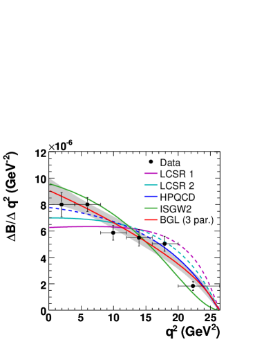
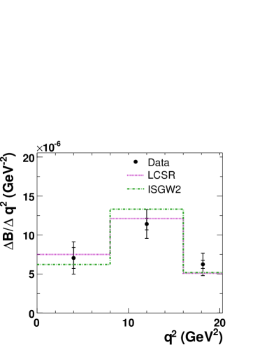
Figure 1: Partial branching fraction of $B^{0}\rightarrow\pi^{-}\ell^{+}\nu$ (left), $B^{0}\rightarrow\rho^{-}\ell^{+}\nu$ (right), in bins of $q^{2}$. Values measured from data (points with errors) are compared with predictions from light cone sum rules (LCSR1 [5] and LCSR2 [6] for $B^{0}\rightarrow\pi^{-}\ell^{+}\nu$, and LCSR [7] for $B^{0}\rightarrow\rho^{-}\ell^{+}\nu$), unquenched lattice QCD (HPQCD [8]), and quark-model (ISGW2 [9]) theory calculations, normalized to equal area. The BGL parameterization [10] is shown with the shaded region indicating the uncertainty on the fitted parameters. For $B^{0}\rightarrow\pi^{-}\ell^{+}\nu$, the dashed lines indicate an extrapolation of the prediction to the full $q^{2}$ range.

The $B\rightarrow\pi\ell\nu$ signal yield is fit in 6 bins of $q^{2}$, and the $B\rightarrow\rho\ell\nu$ yield is measured in 3 bins of $q^{2}$, as shown in Figure 1, after correction for efficiency, detector resolution, bremsstrahlung, and radiative effects. The measured $\Delta{\cal B}/\Delta q^{2}$ distribution is compared with several theoretical form-factor calculations. For $B^{0}\rightarrow\pi^{-}\ell^{+}\nu$ the agreement with the data is best for the HPQCD lattice calculation [8], but the lattice QCD predictions are only valid for $q^{2}>16\mathrm{\,Ge\kern-1.00006ptV}^{2}$, the earlier light cone sum rules (LCSR) calculation (LCSR 1 [5]) for $q^{2}<16\mathrm{\,Ge\kern-1.00006ptV}^{2}$, and the more recent LCSR calculation (LCSR 2 [6]) for $q^{2}<12\mathrm{\,Ge\kern-1.00006ptV}^{2}$. For $B^{0}\rightarrow\rho^{-}\ell^{+}\nu$, the branching fraction measurements are not precise enough to discriminate between the predictions from LCSR [7] and the ISGW2 quark-model calculation [9].

4 Determination of $|V_{ub}|$

The value of $|V_{ub}|$ can be determined from the measured partial branching fraction over a limited range of $q^{2}$ and an integral of the form factor over the same range of $q^{2}$:

$$|V_{ub}|=\sqrt{\frac{\Delta{\cal B}(q^{2}_{min},q^{2}_{max})}{\tau_{0}\ \Delta\zeta(q^{2}_{min},q^{2}_{max})}}\ ,\hskip 42.67912pt\Delta\zeta(q^{2}_{min},q^{2}_{max})=\frac{G^{2}_{F}}{24\pi^{3}}\int\limits_{q^{2}_{min}}^{q^{2}_{max}}p_{\pi}^{3}|f_{+}(q^{2})|^{2}dq^{2}\ ,$$

where $\tau_{0}=(1.530\pm 0.009)$ ps is the $B^{0}$ lifetime.

$|V_{ub}|$ is determined from form-factor theoretical predictions from light cone sum rules at low $q^{2}$ and lattice QCD at high $q^{2}$, and in each case the theoretical uncertainty of about 15% dominates. These measurements of $|V_{ub}|$ are shown in the first three lines of Table 1.

	$q^{2}$ Range	$\Delta{\cal B}$	$\Delta\zeta$	$|V_{ub}|$
	($\mathrm{\,Ge\kern-1.00006ptV}^{2}$)	(10-4)	(ps-1)	(10-3)
LCSR 1 [5]	$0-16$	$1.10\pm 0.07$	$5.44{\pm}1.43$	$3.63\pm 0.12^{+0.59}_{-0.40}$
LCSR 2 [6]	$0-12$	$0.88\pm 0.06$	$4.00^{+1.01}_{-0.95}$	$3.78\pm 0.13^{+0.55}_{-0.40}$
HPQCD [8]	$16-26.4$	$0.32\pm 0.03$	$2.02{\pm}0.55$	$3.21\pm 0.17^{+0.55}_{-0.36}$
FNAL/MILC [11]	$0-26.4$	$1.41\pm 0.09$	—	$2.95\pm 0.31$
HPQCD [8]	$0-26.4$	$1.41\pm 0.09$	—	$2.99\pm 0.35$

Table 1: $|V_{ub}|$ derived from $B\rightarrow\pi\ell\nu$ decays for various $q^{2}$ regions and form-factor calculations. The first three values use data points from only a limited $q^{2}$ range, while the final two values use data from the full $q^{2}$ range. Experimental and theoretical errors on $|V_{ub}|$ are listed separately for partial-$q^{2}$ determinations and combined into a single error for the full-$q^{2}$ determinations.

$|V_{ub}|$ can also be determined using a combined fit to data and theoretical predictions over the full range of $q^{2}$. Three fit parameters describe a quadratic polynomial in the BGL form-factor ansatz [10], and a fourth parameter defines the relative normalization of theory and data, which is proportional to $|V_{ub}|$. The advantage of this method is that it reduces the theoretical uncertainty. The relative error contributions are $3\%$ from the branching-fraction measurement, $5\%$ from the shape of the $q^{2}$ spectrum determined from data, and $8.5\%$ from the form-factor normalization obtained from theory. The result of this fit is shown in Figure 2, and the values of $|V_{ub}|$ for two lattice form-factor calculations are shown in the last two lines of Table 1. Unfortunately, the lattice calculations are only valid at high $q^{2}$, where the decay rate is lowest and the experimental uncertainties are largest.

In summary, $|V_{ub}|$ has been determined with two methods. Using data from a limited $q^{2}$ range, larger values of $|V_{ub}|$ are found with theory predictions for low $q^{2}$ than with predictions for high $q^{2}$. A combined fit to theory and data from the full $q^{2}$ range reduces the overall error by a factor of two. The value of $|V_{ub}|$ from both methods is smaller than most determinations of $|V_{ub}|$ based on inclusive $B\rightarrow X_{u}\ell\nu$ decays, which are in the range $(4.0-4.5)\times 10^{-3}$.

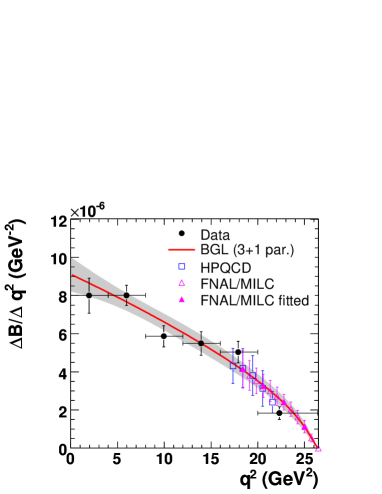
Figure 2: Partial branching fraction of $B^{0}\rightarrow\pi^{-}\ell^{+}\nu$ in bins of $q^{2}$, with the combined fit to data (black points) and lattice theory (squares or triangles) represented by the solid red line. Not all theory points are used because of large correlations. The shaded region indicates the uncertainty on the fitted parameters.

References

- [1] P. del Amo Sanchez et al. [BABAR Collaboration], arXiv:1005.3288 [hep-ex], accepted for publication by Phys. Rev. D.
- [2] BABAR Collaboration, B. Aubert et al., Nucl. Instr. and Methods A479, 1 (2002).
- [3] D. J. Lange, Nucl. Instr. and Methods A462, 152 (2001).
- [4] R. J. Barlow and C. Beeston, Comput. Phys. Commun. 77, 219–228 (1993).
- [5] P. Ball and R. Zwicky, JHEP 0110, 019 (2001); Phys. Rev. D71, 014015 (2005).
- [6] G. Duplancic, A. Khodjamirian, T. Mannel, B. Melic and N. Offen, JHEP 804, 14 (2008).
- [7] P. Ball and V. M. Braun, Phys. Rev. D58, 094016 (1998); P. Ball and R. Zwicky, Phys. Rev. D71, 014029 (2005).
- [8] HPQCD Collaboration, E. Gulez, et al., Phys. Rev. D73, 074502 (2006) and Erratum ibid. D75, 119906 (2007).
- [9] N. Isgur, D. Scora, B. Grinstein, and M. B. Wise, Phys. Rev. D39, 799 (1989); D. Scora, N. Isgur, Phys. Rev. D52, 2783 (1995).
- [10] C. G. Boyd, B. Grinstein, and R.F. Lebed, Phys. Rev. Lett. 74, 4603 (1995); C.G. Boyd and M.J. Savage, Phys. Rev. D56, 303 (1997).
- [11] Fermilab Lattice and MILC Collaboration, J. Bailey et al., Phys. Rev. D79, 054507 (2009).