Supersymmetry Transformations for Delta Potentials

Supersymmetry Transformations for Delta Potentials

David J. FERNÁNDEZ C. ^†, Manuel GADELLA ^‡ and Luis Miguel NIETO ^‡

D.J. Fernández C., M. Gadella and L.M. Nieto

^† Departamento de Física, Cinvestav, AP 14-740, 07000 México DF, Mexico david@fis.cinvestav.mx

^‡ Departamento de Física Teórica, Atómica y Optica, Facultad de Ciencias,
^‡ 47041 Valladolid, Spain manuelgadella1@gmail.com, luismi@metodos.fam.cie.uva.es

Received November 30, 2010, in final form March 19, 2011; Published online March 22, 2011

We make a detailed study of the first and second-order SUSY partners of a one-dimensional free Hamiltonian with a singular perturbation proportional to a Dirac delta function. It is shown that the second-order transformations increase the spectral manipulation possibilities offered by the standard first-order supersymmetric quantum mechanics.

first and second-order SUSY; singular potentials

81Q60

1 Introduction

The study of one-dimensional Hamiltonians with a point interaction has received renewed attention during the past two decades [2, 3, 4, 5, 6, 7, 8]. In general, a point interaction is described by a potential concentrated either in a single or a discrete number of points as it happens, e.g., for the Dirac delta or its derivative. Mathematically, in order to define these potentials, we use the theory of extensions of symmetric operators with equal deficiency indices. These extensions have domains which are characterized by some matching conditions for the wave functions at the points supporting the interaction [3, 9, 10, 11, 12]. In particular, the Dirac delta barrier or well have been extensively studied in this way with or without other interactions [13], with or without mass discontinuities at the singular points etc. [14, 15].

On the other hand, supersymmetric quantum mechanics (SUSY QM) has emerged as the standard technique for generating new potentials with known spectra departing from an initial one [16, 17, 18, 19, 20, 21, 22, 23, 24, 25, 26, 27, 28, 29, 30, 31, 32, 33, 34, 35, 36, 37, 38, 39, 40, 41, 42]. The method has been applied successfully to regular one-dimensional potentials defined on the full real line [43, 44], on the positive semi-axis [45, 46] or in a finite interval [47]. Although there are some works dealing with SUSY QM applied to point potentials [48, 49, 50, 51, 52, 53, 54], however the corresponding study has been done just for particular first-order SUSY transformations, without analyzing the full possibilities of spectral manipulation offered by the method. It is interesting to note as well that a point potential may appear as hidden supersymmetries [55, 56].

Now, it is the appropriate time for studying the behavior of point potentials with bound states under SUSY QM. Due to the calculation complexity, we shall focus our attention to first and second-order transformations, which anyway are interesting by themselves [57, 58, 59, 60]. We shall restrict the discussion to the following one-dimensional Hamiltonian

$$H_{0}=-\frac{1}{2}\,\frac{d^{2}}{dx^{2}}+V_{0}(x),\qquad V_{0}(x):=-a\delta(x),\qquad a>0,$$ (1)

which is mathematically well defined and self-adjoint provided that we use as its domain $\cal D$ the subspace of the Sobolev space $W^{2}_{2}({\mathbb{R}}/\{0\})$ such that for any $\psi(x)\in\cal D$, one has:

$$\left(\begin{array}[]{c}\psi(0+)\\[8.61108pt] \psi^{\prime}(0+)\end{array}\right)=\left(\begin{array}[]{cc}1&0\\[8.61108pt] -2a&1\\ \end{array}\right)\left(\begin{array}[]{c}\psi(0-)\\[8.61108pt] \psi^{\prime}(0-)\\ \end{array}\right),$$ (8)

where $\psi(0+)$, $\psi^{\prime}(0+)$ and $\psi(0-)$, $\psi^{\prime}(0-)$ are the right and left limits of $\psi(x)$, $\psi^{\prime}(x)$ at the origin respectively [3].

In order to achieve our goal, we have organized this paper as follows: in Section 2, we will study the solutions of the stationary Schrödinger equation for the Hamiltonian $H_{0}$ given by (1). In Section 3 we will apply the first-order SUSY techniques, in Section 4 we will analyse the second-order transformations and in Section 5 we will present our conclusions.

2 Solution of the Schrödinger equation

Let us evaluate in the first place the general solution of the stationary Schrödinger equation for an arbitrary $\epsilon=-k^{2}/2<0$:

$$H_{0}u(x)=\epsilon u(x),$$ (9)

with $H_{0}$ given in (1). There is one solution vanishing for $x\rightarrow-\infty$, denoted $u_{+}(x)$, of the form

$$u_{+}(x)=e^{kx}H(-x)+(\alpha\,e^{kx}+\beta e^{-kx})H(x),\qquad k>0,$$ (10)

where $H(x)$ is the Heaviside step function, and $\alpha$, $\beta$ are constants to be determined from the discontinuity equations (8). We need as well the derivative of $u_{+}(x)$,

$$u^{\prime}_{+}(x)=ku_{+}(x)-2k\beta e^{-kx}H(x)+(\alpha+\beta-1)\delta(x).$$ (11)

From equations (10) and (11) it turns out that

$$u_{+}(0+)=\alpha+\beta,\qquad u_{+}(0-)=1,\qquad u_{+}^{\prime}(0+)=k(\alpha-\beta),\qquad u_{+}^{\prime}(0-)=k.$$ (12)

On the other hand, using equations (8) and (12), we obtain:

$$\alpha+\beta=1,\qquad\alpha-\beta=1-2\tilde{a},$$

where $\tilde{a}=a/k$. Hence:

$$\alpha=1-\tilde{a},\qquad\beta=\tilde{a}.$$

Inserting these expressions in equations (10) and (11), we finally get

$$u_{+}(x)=e^{kx}-\tilde{a}\big{(}e^{kx}-e^{-kx}\big{)}H(x),$$ (13)

$$u^{\prime}_{+}(x)=ku_{+}(x)-2ae^{-kx}H(x).$$

Note that the Hamiltonian $H_{0}$ in equation (1) is invariant under the change $x\rightarrow-x$. Thus, we can find a second linearly independent solution $u_{-}(x)$ for the same $\epsilon=-k^{2}/2$, vanishing now for $x\rightarrow\infty$, by applying this transformation to $u_{+}(x)$:

$$u_{-}(x)=\tilde{a}\big{(}e^{kx}-e^{-kx}\big{)}H(-x)+e^{-kx}.$$ (14)

Moreover:

$$u^{\prime}_{-}(x)=-ku_{-}(x)+2ae^{kx}H(-x).$$

Finally, the general solution of equation (9) for $\epsilon=-k^{2}/2<0$ is a linear combination of both (13) and (14) which, up to an unessential constant factor, becomes:

$$u(x)=u_{+}(x)+Du_{-}(x)=e^{kx}+De^{-kx}-\tilde{a}\big{(}e^{kx}-e^{-kx}\big{)}\left[H(x)-DH(-x)\right],$$ (15)

where $D$ is a constant. The corresponding derivative is given by:

$$u^{\prime}(x)=-ku(x)+2ke^{kx}\left[1-\tilde{a}H(x)+D\tilde{a}H(-x)\right].$$ (16)

Note that, up to normalization, both solutions $u_{\pm}(x)$ lead to the same bound state for $k_{0}=a$:

$$\psi_{0}(x)=\sqrt{a}\big{[}e^{k_{0}x}H(-x)+e^{-k_{0}x}H(x)\big{]}.$$

The corresponding eigenvalue becomes

$$E_{0}=-\frac{a^{2}}{2},$$

which coincides with the result derived in [12].

On the other hand, the scattering states for $\epsilon=\kappa^{2}/2>0$ can be simply obtained from the solutions given in equations (13), (14) by the substitution $k\rightarrow-i\kappa$, $\kappa>0$. In particular, for a probability flux approaching the singularity from $-\infty$ the corresponding scattering state arises in this way from the $u_{-}(x)$ of equation (14), which (up to unessential constant factor) leads to

$$\psi(x)=\left[e^{i\kappa x}+\frac{ia}{\kappa-ia}e^{-i\kappa x}\right]H(-x)+\frac{\kappa}{\kappa-ia}e^{i\kappa x}H(x).$$ (17)

It is clear now that the reflection $R$ and transmition $T$ coefficients become the standard ones (see, e.g., [61]):

$$R=\left|\frac{ia}{\kappa-ia}\right|^{2}=\frac{a^{2}}{\kappa^{2}+a^{2}},\qquad T=\left|\frac{\kappa}{\kappa-ia}\right|^{2}=\frac{\kappa^{2}}{\kappa^{2}+a^{2}}.$$ (18)

3 First-order SUSY transformations

Let us start with the initial Schrödinger Hamiltonian $H_{0}$ given in (1). As it is well known (see, e.g., [38, 42] and the references cited there), its first-order SUSY partner,

$$H_{1}=-\frac{1}{2}\frac{d^{2}}{dx^{2}}+V_{1}(x),$$

is intertwined with $H_{0}$ in the way

$$H_{1}A_{1}^{+}=A_{1}^{+}H_{0},$$ (19)

where

$$A_{1}^{+}=\frac{1}{\sqrt{2}}\left(-\frac{d}{dx}+\frac{u^{\prime}}{u}\right).$$

Here, the transformation function $u(x)$ is the seed solution given in (15), associated to the factorization energy $\epsilon=-k^{2}/2$ and satisfying equation (9). The SUSY partner potential $V_{1}(x)$ of $V_{0}(x)$ is given by:

$$V_{1}(x)=V_{0}(x)-[\ln u(x)]^{\prime\prime}.$$ (20)

We assume the standard restriction $\epsilon\leq E_{0}\Rightarrow k\geq k_{0}$, in order to avoid the creation of new singularities in $V_{1}(x)$ with respect to those of $V_{0}(x)$. Note that, from equation (20) and (9) we have:

$$V_{1}(x)=V_{0}(x)-\frac{u^{\prime\prime}(x)}{u(x)}+\left[\frac{u^{\prime}(x)}{u(x)}\right]^{2}=-V_{0}(x)+2\epsilon+\left[\frac{u^{\prime}(x)}{u(x)}\right]^{2}.$$ (21)

Hence, a straightforward calculation using equations (15), (16) leads to:

$$\left[\frac{u^{\prime}(x)}{u(x)}\right]^{2}=k^{2}-\frac{4k^{2}(1-\tilde{a})}{u^{2}(x)}\big{[}D+\tilde{a}D^{2}H(-x)+\tilde{a}H(x)\big{]}.$$ (22)

As $\epsilon=-k^{2}/2$, equations (21), (22) give:

$$V_{1}(x)=a\delta(x)-\frac{4k^{2}(1-\tilde{a})[D+\tilde{a}D^{2}H(-x)+\tilde{a}H(x)]}{\{e^{kx}+De^{-kx}+2\tilde{a}\sinh(kx)[DH(-x)-H(x)]\}^{2}}.$$ (23)

Note that the denominator of equation (23) never vanishes for $x\in(-\infty,\infty)$ and $D\geq 0$. Moreover, it can be seen that the delta term in $V_{1}(x)$ is now repulsive (since $a>0$).

A straightforward consequence of the intertwining relationship (19) is that for any eigenfunction $\psi$ of $H_{0}$ associated to the eigenvalue $E$ ($H_{0}\psi=E\psi$) such that $A_{1}^{+}\psi\neq 0$, it turns out that $\psi^{(1)}\propto A_{1}^{+}\psi\propto W(u,\psi)/u$ is a corresponding eigenfunction of $H_{1}$ associated to $E$. Moreover, if $\psi$ satisfies as well equation (8) it turns out that $\psi^{(1)}$ now obeys:

$$\left(\begin{array}[]{c}\psi^{(1)}(0+)\\ {\psi^{(1)}}^{\prime}(0+)\end{array}\right)=\left(\begin{array}[]{cc}1&0\\ 2a&1\end{array}\right)\left(\begin{array}[]{c}\psi^{(1)}(0-)\\ {\psi^{(1)}}^{\prime}(0-)\end{array}\right),$$

which is consistent with the fact that the intensity of the delta term in $V_{1}(x)$ has an opposite sign compared with $V_{0}(x)$ and the second term of $V_{1}(x)$ has just a finite discontinuity at $x=0$ (see equation (23)).

Concerning the spectrum of $H_{1}$, let us note in the first place that $A_{1}^{+}$ transforms the scattering eigenfunctions of $H_{0}$ into the corresponding ones of $H_{1}$. In particular, the wavefunction $\psi(x)$ given in equation (17), when transformed by acting on it with $A_{1}^{+}$, produces an expression $\psi^{(1)}(x)$ which is a bit large to be presented here. However, for large values of $|x|$ that expression reduces to the following scattering one (up to a constant factor):

$$\psi^{(1)}(x)\underset{|x|\rightarrow\infty}{\rightarrow}\left[e^{i\kappa x}+\left(\frac{a}{a+i\kappa}\right)\left(\frac{-k+i\kappa}{k+i\kappa}\right)e^{-i\kappa x}\right]H(-x)$$

$$\hphantom{\psi^{(1)}(x)\underset{|x|\rightarrow\infty}{\rightarrow}}{}+\left(\frac{i\kappa}{a+i\kappa}\right)\left(\frac{-k+i\kappa}{k+i\kappa}\right)e^{i\kappa x}H(x).$$

This means that the initial reflection and transmission coefficients are unchanged under the first-order SUSY transformation (compare equation (18)). We thus conclude that the continuous spectrum of $H_{0}$ belongs as well to the spectrum of $H_{1}$.

Let us note that the differences in the spectra of $H_{1}$ and $H_{0}$ rely in general in the modifications produced by a non-singular SUSY transformation on the discrete part of the initial spectrum. For first-order transformations, these changes can be classified according to the essentially different combinations of the parameters $D\geq 0$ and $k\geq k_{0}$ which characterize the seed eigenfunction $u(x)$. We can find three different situations.

1. Creation of a new ground state at $\epsilon<E_{0}$. This case appears for $D>0$, $k>k_{0}$. Here, the eigenfunction $\psi_{\epsilon}^{(1)}\propto 1/u(x)$ of $H_{1}$ associated to $\epsilon$ is square-integrable. Moreover, since the mapped initial ground state $\psi_{0}^{(1)}=\frac{1}{\sqrt{2}}\frac{1}{\sqrt{E_{0}-\epsilon}}\frac{W(u,\psi_{0})}{u}$ is as well a normalized eigenfunction of $H_{1}$ with eigenvalue $E_{0}$, then Sp$(H_{1})=\{\epsilon,E_{0}\}\cup[0,\infty)=\{\epsilon\}\cup{\rm Sp}(H_{0})$.

2. Isospectral transformations. These are achieved from the previous case either by taking $D\rightarrow 0$ or $D\rightarrow\infty$. Since in both situations $u(x)$ goes to zero at one of the ends of the $x$-domain, it turns out that $\psi_{\epsilon}^{(1)}\propto 1/u(x)$ is no longer square-integrable, although $\psi_{0}^{(1)}$ is. Thus, Sp$(H_{1})=\{E_{0}\}\cup[0,\infty)={\rm Sp}(H_{0})$.

3. Deleting $E_{0}$. This situation arises from the previous one by taking $k\!=\!k_{0}\!=\!a$ ($\tilde{a}\!=\!a/k\!=\!1$). Since $u(x)\propto\psi_{0}(x)$ is square-integrable, then $\psi_{\epsilon}^{(1)}\propto 1/u(x)$ is not normalizable, and then Sp$(H_{1})=[0,\infty)$. From equation (23), it is clear that now

   $$V_{1}(x)=a\delta(x).$$ (24)

   This means that, by deleting the bound state of the attractive delta well $V_{0}(x)=-a\delta(x)$, $a>0$, which is placed at $E_{0}=-a^{2}/2$, we recover the repulsive delta barrier of equation (24), a standard result well known in the literature.

4 Second-order SUSY transformations

In this section it will be illustrated, by means of the delta-well potential, the advantages for manipulating spectra of the second-order SUSY transformations [57, 58, 59, 60] compared with the first-order ones. It is nowadays known that the second-order SUSY partners $H_{2}$ of the initial Hamiltonian $H_{0}$ can be generated either by employing two eigenfunctions $u_{1}(x)$, $u_{2}(x)$ of $H_{0}$, not necessarily physical, associated to two different factorization energies $\epsilon_{1,2}$, $\epsilon_{1}\neq\epsilon_{2}$ [38, 42] or by an appropriate eigenfunction $u_{1}(x)$ in the limit when $\epsilon_{2}\rightarrow\epsilon_{1}$ (the so called confluent case [62, 63]). In both situations the two Hamiltonians $H_{0}$, $H_{2}$ are intertwined by a second-order operator in the way

$$H_{2}B_{2}^{+}=B_{2}^{+}H_{0},$$

where

$$B_{2}^{+}=\frac{1}{2}\left(-\frac{d}{dx}+\frac{{u_{2}^{(1)}}^{\prime}}{u_{2}^{(1)}}\right)\left(-\frac{d}{dx}+\frac{u_{1}^{\prime}}{u_{1}}\right),\qquad u_{2}^{(1)}=\frac{w(x)}{u_{1}(x)},$$

the new Hamiltonian $H_{2}$ takes the standard Schrödinger form

$$H_{2}=-\frac{1}{2}\frac{d^{2}}{dx^{2}}+V_{2}(x),$$

and the second-order SUSY partner $V_{2}(x)$ of the initial potential $V_{0}(x)$ is given by

$$V_{2}(x)=V_{0}(x)-[\ln w(x)]^{\prime\prime},$$ (25)

the real function $w(x)$ being proportional in general to the Wronskian of two generalized eigenfunctions of $H_{0}$ [64]. An explicit classification of the several second-order SUSY transformations is next given.

4.1 Confluent case [62, 63]

Let us consider in the first place the limit $\epsilon_{2}\rightarrow\epsilon_{1}\equiv\epsilon=-k^{2}/2<0$, taking as seed the Schrödinger solution $u_{+}(x)$ vanishing as $x\longmapsto-\infty$, which means to take the $u(x)$ given in equation (15) with $D=0$, namely:

$$u(x)=e^{kx}-2\tilde{a}\sinh(kx)H(x).$$ (26)

In this case the real function $w(x)$ appearing in equation (25) takes the form [63]

$$w(x):=w_{0}+\int_{-\infty}^{x}u^{2}(y)\,dy.$$

An explicit calculation for $x\leq 0$ leads to:

$$\int_{-\infty}^{x}u^{2}(y)\,dy=\int_{-\infty}^{x}e^{2ky}\,dy=\frac{e^{2kx}}{2k}.$$

On the other hand, for $x>0$ it turns out that:

$$\int_{-\infty}^{x}u^{2}(y)\,dy=\int_{-\infty}^{0}u^{2}(y)\,dy+\int_{0}^{x}u^{2}(y)\,dy$$

$$\hphantom{\int_{-\infty}^{x}u^{2}(y)\,dy}{}=\frac{\tilde{a}}{k}+\frac{(1-2\tilde{a})}{2k}\,e^{2kx}+\frac{\tilde{a}^{2}}{k}\,\sinh(2kx)+2\tilde{a}(1-\tilde{a})x.$$

By combining these two results, we obtain

$$w(x)=w_{0}+\frac{e^{2kx}}{2k}+\left[\frac{\tilde{a}}{k}-\frac{\tilde{a}}{k}e^{2kx}+\frac{\tilde{a}^{2}}{k}\sinh(2kx)+2\tilde{a}(1-\tilde{a})x\right]H(x).$$ (27)

The second-order SUSY partner potential of $V_{0}(x)$ becomes now

$$V_{2}(x)=-a\delta(x)+\frac{u^{4}(x)}{w^{2}(x)}-\frac{2u(x)u^{\prime}(x)}{w(x)}.$$ (28)

Note that, since $u^{\prime}(0+)=k-2a$ and $u^{\prime}(0-)=k$, then $u^{\prime}(x)$ and consequently the potential difference $\Delta V(x)=V_{2}(x)-V_{0}(x)$ have a finite discontinuity at $x=0$.

In order to avoid the arising of extra singularities for $V_{2}(x)$ with respect to $V_{0}(x)$ we have to take $w_{0}\geq 0$. Concerning the spectrum of $H_{2}$, a similar calculation as in the first-order case shows that the scattering eigenfunctions of $H_{0}$ are mapped into the corresponding ones of $H_{2}$, i.e., the energy interval $[0,\infty)$ belongs to Sp$(H_{2})$. As for the discrete part of the spectrum, several possibilities of spectral manipulation emerge, according to how we choose $k$ and $w_{0}$.

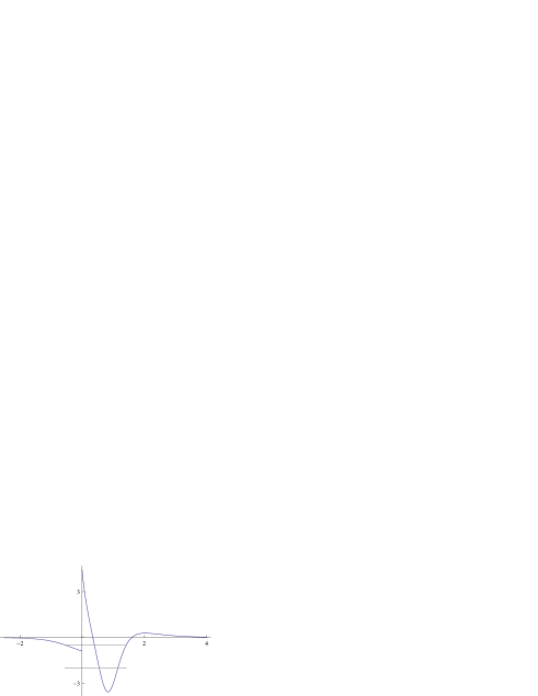
Figure 1: Potential difference $\Delta V(x)$ as function of $x$ (blue lines) induced by the confluent second order SUSY transformation for $a=2$, $k=1$, $w_{0}=1$. A new level was created at $\epsilon=-1/2$, above the initial ground state $E_{0}=-2$ (gray horizontal lines).

1. Creating a new bound state at $\epsilon\neq E_{0}$. This case appears by taking $w_{0}>0$ and $k\neq k_{0}=a$. Since

   $$\lim_{|x|\rightarrow\infty}\psi_{\epsilon}^{(2)}\propto\lim_{|x|\rightarrow\infty}\frac{u(x)}{w(x)}\propto e^{-k|x|},$$

   the eigenfunction $\psi_{\epsilon}^{(2)}$ of $H_{2}$ associated to $\epsilon$ is square-integrable, i.e., a new bound state has been created at $\epsilon$, either below the ground state for $k>k_{0}$ or above it for $k<k_{0}$. The last option is illustrated in Fig. 1, where we have plotted the potential difference $\Delta V(x)$ as a function of $x$ for $a=2$, $k=1$, $w_{0}=1$, i.e., a new level was created at $\epsilon=-1/2>E_{0}=-2$ (see the two gray horizontal lines in the same graph). Note the existence of a finite discontinuity in $\Delta V(x)$ at $x=0$, induced by a similar discontinuity of $u^{\prime}(x)$ at the same point.

2. Isospectral transformations. They arise in the first place as a limit of the previous case for $\epsilon\neq E_{0}$ and $w_{0}\rightarrow 0$. Note that the long explicit expression for the $V_{2}(x)$ of (28) which would appear if we would substitute explicitly the $u(x)$ and $w(x)$ of equations (26), (27) becomes strongly simplified in this limit:

   $$V_{2}(x)=-a\delta(x)+H(x)\Big{(}\!8\tilde{a}k^{2}e^{2kx}[(\tilde{a}-1)e^{2kx}-\tilde{a}]\{(\tilde{a}-1)[2kx(\tilde{a}-1)+1-2\tilde{a}]e^{2kx}$$

   $$\hphantom{V_{2}(x)=}{}+\tilde{a}[2kx(\tilde{a}-1)+2\tilde{a}-3]\}\!\Big{)}\!\Big{/}\!\big{\{}(\tilde{a}-1)^{2}e^{4kx}\!+2\tilde{a}[1-2kx(\tilde{a}-1)]e^{2kx}\!-\tilde{a}^{2}\big{\}}^{2}.$$

   Since now

   $$\lim_{x\rightarrow-\infty}\frac{u(x)}{w(x)}=\infty,$$

   it turns out that $\epsilon\not\in{\rm Sp}(H_{2})=\{E_{0}\}\cup[0,\infty)={\rm Sp}(H_{0})$.

   An alternative way to produce isospectral transformations is to use the single bound state of $H_{0}$ for evaluating $w(x)$. The corresponding formula is achieved from equation (27) by taking $k=k_{0}=a$, $\tilde{a}=1$, which leads to:

   $$w(x)=w_{0}+\frac{e^{2ax}}{2a}-\frac{2}{a}\sinh^{2}(ax)H(x)\,.$$ (29)

   Hence

   $$V_{2}(x)=-a\delta(x)-\frac{8w_{0}a^{3}e^{2ax}}{(2w_{0}a+e^{2ax})^{2}}H(-x)+\frac{8a^{2}e^{2ax}(1+w_{0}a)}{[2(1+w_{0}a)e^{2ax}-1]^{2}}H(x).$$ (30)

   Note that now $w(x)$ does not have any node for

   $$w_{0}\in\left(-\infty,-\frac{1}{a}\right)\cup\left(0,\infty\right).$$

   Moreover, in this domain it turns out that

   $$\lim_{|x|\rightarrow\infty}\frac{u(x)}{w(x)}\propto e^{-a|x|},$$

   i.e., $\psi_{\epsilon}^{(2)}\propto u(x)/w(x)$ is square-integrable $\Rightarrow$ ${\rm Sp}(H_{2})=\{E_{0}\}\cup[0,\infty)={\rm Sp}(H_{0})$.

3. Deleting the ground state of $H_{0}$. By taking now the limit of equation (29) for $w_{0}\rightarrow 0$ or $w_{0}\rightarrow-1/a$, it turns out that $\lim\limits_{x\rightarrow-\infty}u(x)/w(x)=\infty$ or $\lim\limits_{x\rightarrow\infty}u(x)/w(x)=\infty$ respectively. In both cases $\psi_{\epsilon}^{(2)}$ is not square-integrable and then

   $$E_{0}\not\in{\rm Sp}(H_{2})=[0,\infty).$$

   This result means that we have deleted the ground state of $H_{0}$ in order to obtain $H_{2}$. For $w_{0}\rightarrow 0$ the potential of equation (30) becomes

   $$V_{2}(x)=-a\delta(x)+\frac{8a^{2}e^{2ax}}{(2e^{2ax}-1)^{2}}H(x).$$ (31)

   On the other hand, for $w_{0}\rightarrow-1/a$ the corresponding potential $V_{2}(x)$ is obtained from the previous one by the change $x\rightarrow-x$.

Let us remark that, although the final spectra of the SUSY partner Hamiltonians of $H_{0}$ are the same when deleting its ground state in the first-order and in the confluent second-order transformations, however the potentials $V_{1}(x)$ and $V_{2}(x)$ are physically different (compare equations (24) and (31)). In particular, note the opposite signs of the coefficients of the Dirac delta function for both potentials.

4.2 Complex case [65, 66, 67]

Let us assume that $k=k_{R}+ik_{I}$ is complex with $k_{R}>0$, $k_{I}\in{\mathbb{R}}$, and suppose that the two involved factorization energies are now given by $\epsilon=-k^{2}/2$ and $\bar{\epsilon}$, where $\bar{z}$ denotes the complex conjugate of $z$. Since we need to avoid the arising of extra singularities in the new potential, we will take a Schrödinger seed solution vanishing at one of the ends of the $x$-domain in the form given in equation (26) with $k\in{\mathbb{C}}$, namely,

$$u(x)=e^{kx}-\frac{2a}{k}\sinh(kx)H(x),\qquad\bar{u}(x)=e^{\bar{k}x}-\frac{2a}{\bar{k}}\sinh(\bar{k}x)H(x).$$ (32)

To compute now the second-order SUSY partner potential $V_{2}(x)$, we have to obtain in the first place the Wronskian $W(u,\bar{u})$ and then the real function

$$w(x)=\frac{W(u,\bar{u})}{2(\epsilon-\bar{\epsilon})}.$$

This calculation is cumbersome but otherwise straightforward, which leads to:

$$w(x)=\frac{e^{2k_{R}x}}{2k_{R}}+\bigg{\{}-\frac{a}{|k|^{2}}\big{[}\cosh(2k_{R}x)-\cos(2k_{I}x)\big{]}$$

$$\phantom{w(x)=}{}+\frac{a(a-k_{R})}{|k|^{2}k_{R}k_{I}}\big{[}k_{I}\sinh(2k_{R}x)-k_{R}\sin(2k_{I}x)\big{]}\bigg{\}}H(x).$$ (33)

Then, $V_{2}(x)$ will be given by

$$V_{2}(x)=-a\delta(x)+\frac{|u(x)|^{4}}{w^{2}(x)}-\frac{[u(x)\bar{u}^{\prime}(x)+\bar{u}(x)u^{\prime}(x)]}{w(x)},$$ (34)

with $u(x)$, $\bar{u}(x)$ and $w(x)$ as given in equations (32) and (33). An illustration of the potential difference $\Delta V(x)$ as function of $x$ for $a=2$, $k=1/100+i/10$ is given in Fig. 2.

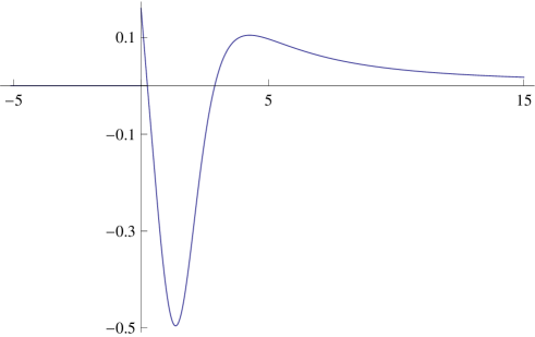
Figure 2: Potential difference $\Delta V(x)$ as function of $x$ induced by the complex second order SUSY transformation for $a=2$, $k=1/100+i/10$. The two potentials $V_{2}(x)$ and $V_{0}(x)$ are isospectral.

Note that these equations become highly simplified if $k_{R}=a$:

$$w(x)=\frac{e^{2ax}}{2a}-\left(\frac{a}{a^{2}+k_{I}^{2}}\right)\left[\cosh(2ax)-\cos(2k_{I}x)\right]H(x),$$ (35)

$$|u(x)|^{2}=e^{2ax}-\left(\frac{2a}{a^{2}+k_{I}^{2}}\right)\left[a\sinh(2ax)+k_{I}\sin(2k_{I}x)\right]H(x).$$ (36)

Moreover, for the particular choice $k_{R}=a$ we get a more compact expression for the new potential $V_{2}(x)$ than for a generic $k_{R}$ that would appear if we would substitute the $u(x)$ and $w(x)$ of equations (32), (33) in equation (34):

$$V_{2}(x)=-a\delta(x)+H(x)\Big{(}\!4a^{2}e^{2ax}[2(a^{2}-k_{I}^{2})\cos(2k_{I}x)(a^{2}-k_{I}^{2}e^{4ax})$$ (37)

$$\hphantom{V_{2}(x)=}{}-4ak_{I}\sin(2k_{I}x)(a^{2}+k_{I}^{2}e^{4ax})+8a^{2}k_{I}^{2}e^{2ax}]\!\Big{)}\!\Big{/}\!\big{[}a^{2}-k_{I}^{2}e^{4ax}-2a^{2}e^{2ax}\cos(2k_{I}x)\big{]}^{2}.$$

Let us remark that, for the general case characterized by equations (32) and (33) as well as the particular ones described by equations (35)–(37), the scattering states of $H_{0}$ are mapped into the corresponding ones of $H_{2}$, and the same happens for the bound state. Thus, it turns out that the spectrum of $H_{2}$ will be equal to ${\rm Sp}(H_{0})=\{E_{0}\}\cup[0,\infty)$, i.e., the complex second-order SUSY transformations which produce a real final potential are strictly isospectral.

4.3 Real case

Let us take now two seed solutions $u_{1}$, $u_{2}$ in the form given in equation (15), associated to the pair of real factorization energies $\epsilon_{2}<\epsilon_{1}\Rightarrow k_{2}>k_{1}$. Their explicit forms, and the corresponding derivatives, are given by:

$$u_{i}(x)=e^{k_{i}x}+D_{i}e^{-k_{i}x}+2\tilde{a}_{i}\sinh(k_{i}x)[D_{i}H(-x)-H(x)],$$ (38)

$$u_{i}^{\prime}(x)=-k_{i}u_{i}(x)+2k_{i}e^{k_{i}x}\left[1-\tilde{a}_{i}H(x)+D_{i}\tilde{a}_{i}H(-x)\right],\qquad i=1,2,$$

where $\tilde{a}_{i}=a/k_{i}$. Similarly as in the complex case, the calculation of the Wronskian $w(x)\equiv W(u_{1},u_{2})$ of the two involved Schrödinger seed solutions is once again cumbersome, but a convenient compact expression reads:

$$w(x)=(k_{1}-k_{2})u_{1}u_{2}+2k_{2}u_{1}e^{k_{2}x}\left[1-\tilde{a}_{2}H(x)+D_{2}\tilde{a}_{2}H(-x)\right]$$

$$\phantom{w(x)=}{}-2k_{1}u_{2}e^{k_{1}x}\left[1-\tilde{a}_{1}H(x)+D_{1}\tilde{a}_{1}H(-x)\right].$$

By employing this equation, it is straightforward to calculate the new potential through:

$$V_{2}(x)=-a\delta(x)+\left(\frac{w^{\prime}}{w}\right)^{2}-\frac{w^{\prime\prime}}{w}=-a\delta(x)+\left[\frac{(k_{1}^{2}-k_{2}^{2})u_{1}u_{2}}{w}\right]^{2}+\frac{(k_{1}^{2}-k_{2}^{2})(u_{1}u_{2}^{\prime}+u_{1}^{\prime}u_{2})}{w}.$$

Concerning the spectrum of $H_{2}$, once again the scattering states of $H_{0}$ are mapped into the corresponding ones of $H_{2}$. As for the discrete part of the spectrum, several possibilities are worth of study.

1. Creating two new levels. Let us suppose first that $\epsilon_{1}\neq E_{0}\neq\epsilon_{2}$. In order that $w(x)$ do not have nodes, the two factorization energies must be placed either both below (for $k_{2}>k_{1}>a$) or both above $E_{0}$ (for $k_{1}<k_{2}<a$). Moreover, according to the chosen ordering $\epsilon_{2}<\epsilon_{1}$, the solution $u_{2}(x)$ must have one extra node with respect to $u_{1}(x)$ [38]. In the domain $k_{2}>k_{1}>a$ ($\epsilon_{2}<\epsilon_{1}<E_{0}$) this can be achieved by taking $D_{2}<0$ and $D_{1}>0$ while for $k_{1}<k_{2}<a$ ($E_{0}<\epsilon_{2}<\epsilon_{1}$) it must be taken $D_{2}>0$ and $D_{1}<0$. With this choice of parameters, it turns out that the two eigenfunctions of $H_{2}$ associated to $\epsilon_{1}$ and $\epsilon_{2}$, $\psi_{\epsilon_{1}}^{(2)}\propto u_{2}/w$ and $\psi_{\epsilon_{2}}^{(2)}\propto u_{1}/w$, are square-integrable. Thus,

   $${\rm Sp}(H_{2})=\{\epsilon_{2},\epsilon_{1}\}\cup{\rm Sp}(H_{0}),$$

   i.e., two new levels have been created for $H_{2}$, either both below the ground state of $H_{0}$ (for $k_{2}>k_{1}>a$) or both above $E_{0}$ (for $k_{1}<k_{2}<a$). An illustration of the last situation is shown in Fig. 3, where we have plotted the potential difference $\Delta V(x)$ for $a=2$, $k_{2}=1$, $k_{1}=1/2$, $D_{1}=-1/2$, $D_{2}=1$. As a result of the transformation, two new levels were created above the ground state energy of $H_{0}$ at the positions $\epsilon_{2}=-1/2$ and $\epsilon_{1}=-1/8$ (see the gray horizontal lines at Fig. 3).

   

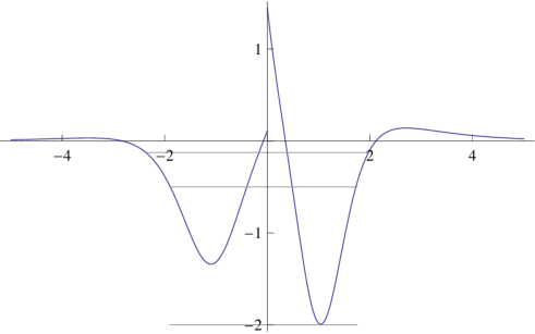
   Figure 3: Potential difference $\Delta V(x)$ as function of $x$ (blue lines), induced by a real second order SUSY transformation for $a=2$, $k_{2}=1$, $k_{1}=1/2$, $D_{1}=-1/2$, $D_{2}=1$. Note that two new levels were created above $E_{0}=-2$, at the positions $\epsilon_{2}=-1/2$ and $\epsilon_{1}=-1/8$ (gray horizontal lines).

2. Creating one new level. This case arises from the previous one for $D_{2}\rightarrow 0$. Now it turns out that $\psi_{\epsilon_{2}}^{(2)}$ is not square-integrable anymore, meaning that

   $${\rm Sp}(H_{2})=\{\epsilon_{1}\}\cup{\rm Sp}(H_{0}).$$

   Thus, in order to generate $H_{2}$ a new level has been created at $\epsilon_{1}$, above $E_{0}$ for $k_{1}<a$ and below it for $k_{1}>a$.

3. Isospectral transformations. These can be achieved from case (i) for $D_{1}=D_{2}\rightarrow 0$, where both $\psi_{\epsilon_{1}}^{(2)}$ and $\psi_{\epsilon_{2}}^{(2)}$ cease to be square-integrable so that $\epsilon_{i}\not\in{\rm Sp}(H_{2})$, $i=1,2$. Hence,

   $${\rm Sp}(H_{2})={\rm Sp}(H_{0}).$$

4. Moving the level $E_{0}$. This procedure is obtained from case (i), e.g., by taking $\epsilon_{2}=E_{0}$, $D_{2}\rightarrow 0$, $u_{2}(x)\propto\psi_{0}(x)$, and $u_{1}(x)$ as given in equation (38) with $D_{1}<0$, $\epsilon_{1}>E_{0}$. With this choice it can be shown that $\psi_{\epsilon_{2}}^{(2)}\propto u_{1}/w$ is not square-integrable but $\psi_{\epsilon_{1}}^{(2)}$ does, meaning that

   $${\rm Sp}(H_{2})=\{\epsilon_{1}\}\cup[0,\infty).$$

   In a way, the level $E_{0}$ has been moved up to $\epsilon_{1}$ for generating $H_{2}$.

5. Deleting the level $E_{0}$. This can be achieved as a limit of the previous case for $D_{1}\rightarrow 0$. Now it turns out that $\lim\limits_{x\rightarrow 0}u_{2}/w=\infty$, i.e., $\epsilon_{1}\not\in{\rm Sp}(H_{2})$, and hence

   $${\rm Sp}(H_{2})=[0,\infty).$$

5 Conclusions

We have employed the first and second-order supersymmetric quantum mechanics for generating new potentials with modified spectra departing from the delta well potential. The first-order transformation allowed us to change just the ground state energy level, while the second-order transformations enlarged the possibilities of spectral control, including the option of manipulating the excited state levels. On the other hand, it is important to remember that the first-order transformations induced in the new potential a delta term with an opposite sign compared with the initial one (physically the delta term changed from attractive to repulsive). Meanwhile, the second-order transformations generated a delta term with exactly the same sign as the initial one (the attractive nature was preserved under the transformation). These physical differences should be taken into account in the determination of the most appropriate transformation for building a potential model. We can conclude that supersymmetric quantum mechanics is a powerful mathematical tool, which is quite useful for implementing the spectral design in physics.

Acknowledgement

Partial financial support is acknowledged to the Spanish Junta de Castilla y León (Project GR224) and the Ministry of Science and Innovation (Projects MTM2009-10751 and FPA2008-04772-E). DJFC acknowledges the support of Conacyt.

References

- [1]
- [2] Seba P., Some remarks on the -interaction in one dimension, Rep. Math. Phys. 24 (1986), 111–120.
- [3] Kurasov P., Distribution theory for discontinuous test functions and differential operators with generalized coefficients, J. Math. Anal. Appl. 201 (1996), 297–323.
- [4] Coutinho F.A.B., Nogami Y., Fernando Perez J., Generalized point interactions in one-dimensional quantum mechanics, J. Phys. A: Math. Gen. 30 (1997), 3937–3945.
- [5] Toyama F.M., Nogami Y., Transmission-reflection problem with a potential of the form of the derivative of the delta function, J. Phys. A: Math. Theor. 40 (2007), F685–F690.
- [6] Fülöp T., Tsutsui I., A free particle on a circle with point interaction, Phys. Lett. A 264 (2000), 366–374, quant-ph/9910062.
- [7] Hejcik P., Cheon T., Irregular dynamics in a solvable one-dimensional quantum graph, Phys. Lett. A 356 (2006), 290–293, quant-ph/0512239.
- [8] Christiansen P.L., Arnbak H.C., Zolotaryuk A.V., Ermakov V.N., Gaididei Y.B., On the existence of resonances in the transmission probability for interactions arising from derivatives of Dirac’s delta function, J. Phys. A: Math. Gen. 36 (2003), 7589–7600.
- [9] Albeverio S., Gesztesy F., Høegh-Krohn R., Holden H., Solvable models in quantum mechanics, Texts and Monographs in Physics, Springer-Verlag, New York, 1988.
- [10] Albeverio S., Kurasov P., Singular perturbations of differential operators. Solvable Schrödinger type operators, London Mathematical Society Lecture Note Series, Vol. 271, Cambridge University Press, Cambridge, 2000.
- [11] Gadella M., Kuru Ş., Negro J., Self-adjoint Hamiltonians with a mass jump: general matching conditions, Phys. Lett. A 362 (2007), 265–268.
- [12] Gadella M., Negro J., Nieto L.M., Bound states and scattering coefficients of the potential, Phys. Lett. A 373 (2009), 1310–1313.
- [13] Fernández C., Palma G., Prado H., Resonances for Hamiltonians with a delta perturbation in one dimension, J. Phys. A: Math. Gen. 38 (2005), 7509–7518.
- [14] Gadella M., Heras F.J.H., Negro J., Nieto L.M., A delta well with a mass jump, J. Phys. A: Math. Theor. 42 (2009), 465207, 11 pages.
- [15] Álvarez J.J., Gadella M., Heras F.J.H., Nieto L.M., A one-dimensional model of resonances with a delta barrier and mass jump, Phys. Lett. A 373 (2009), 4022–4027.
- [16] Witten E., Dynamical breaking of supersymmetry, Nuclear Phys. B 185 (1981), 513–554.
- [17] Mielnik B., Factorization method and new potentials with the oscillator spectrum, J. Math. Phys. 25 (1984), 3387–3389.
- [18] Fernández D.J., New hydrogen-like potentials, Lett. Math. Phys. 8 (1984), 337–343, quant-ph/0006119.
- [19] Andrianov A.A., Borisov N.V., Ioffe M.V., Quantum systems with identical energy spectra, JETP Lett. 39 (1984), 93–97.
- [20] Andrianov A.A., Borisov N.V., Ioffe M.V., The factorization method and quantum systems with equivalent energy spectra, Phys. Lett. A 105 (1984), 19–22.
- [21] Sukumar C.V., Supersymmetric quantum mechanics of one-dimensional systems, J. Phys. A: Math. Gen. 18 (1985), 2917–2936.
- [22] Sukumar C.V., Supersymmetric quantum mechanics and the inverse scattering method, J. Phys. A: Math. Gen. 18 (1985), 2937–2955.
- [23] Sukumar C.V., Supersymmetry, potentials with bound states at arbitrary energies and multi-soliton configurations, J. Phys. A: Math. Gen. 19 (1986), 2297–2316.
- [24] Sukumar C.V., Supersymmetry and potentials with bound states at arbitrary energies. II, J. Phys. A: Math. Gen. 20 (1987), 2461–2481.
- [25] Beckers J., Dehin D., Hussin V., Symmetries and supersymmetries of the quantum harmonic oscillator, J. Phys. A: Math. Gen. 20 (1987), 1137–1154.
- [26] Alves N.A., Drigo Filho E., The factorization method and supersymmetry, J. Phys. A: Math. Gen. 21 (1988), 3215–3225.
- [27] Lahiri A., Roy P.K., Bagchi B., Supersymmetry in quantum mechanics, Internat. J. Modern Phys. A 5 (1990), 1383–1456.
- [28] Roy B., Roy P., Roychoudhury R., On solutions of quantum eigenvalue problems: a supersymmetric approach, Fortschr. Phys. 39 (1991), 211–258.
- [29] de Lange O.L., Raab R.E., Operator methods in quantum mechanics, The Clarendon Press, Oxford University Press, New York, 1991.
- [30] Baye D., Phase-equivalent potentials for arbitrary modifications of the bound spectrum, Phys. Rev. A 48 (1993), 2040–2047.
- [31] Sparenberg J.-M., Baye D., Supersymmetric transformations of real potentials on the line, J. Phys. A: Math. Gen. 28 (1995), 5079–5095.
- [32] Bagchi B., Supersymmetry in quantum and classical mechanics, Chapman & Hall/CRC Monographs and Surveys in Pure and Applied Mathematics, Vol. 116. Chapman & Hall/CRC, Boca Raton, FL, 2001.
- [33] Cooper F., Khare A., Sukhatme U., Supersymmetry in quantum mechanics, World Scientific Publishing Co., Inc., River Edge, NJ, 2001.
- [34] Mielnik B., Rosas-Ortiz O., Factorization: little or great algorithm?, J. Phys. A: Math. Gen. 37 (2004), 10007–10035.
- [35] Andrianov A.A., Cannata F., Nonlinear supersymmetry for spectral design in quantum mechanics, J. Phys. A: Math. Gen. 37 (2004), 10297–10321, hep-th/0407077.
- [36] Plyushchay M., Nonlinear supersymmetry: from classical to quantum mechanics, J. Phys. A: Math. Gen. 37 (2004), 10375–10384, hep-th/0402025.
- [37] Sukumar C.V., Supersymmetric quantum mechanics and its applications, AIP Conf. Proc. 744 (2005), 166–235.
- [38] Fernández D.J., Fernández-García N., Higher-order supersymmetric quantum mechanics, AIP Conf. Proc. 744 (2005), 236–273, quant-ph/0502098.
- [39] Dong S.-H., Factorization method in quantum mechanics, Fundamental Theories of Physics, Vol. 150, Springer, Dordrecht, 2007.
- [40] Andrianov A.A., Sokolov A.V., Factorization of nonlinear supersymmetry in one-dimensional quantum mechanics. I. General classification of reducibility and analysis of the third-order algebra, J. Math. Sci. 143 (2007), 2707–2722, arXiv:0710.5738.
- [41] Sokolov A.V., Factorization of nonlinear supersymmetry in one-dimensional quantum mechanics. II. Proofs of theorems on reducibility, J. Math. Sci. 151 (2008), 2924–2936, arXiv:0903.2835.
- [42] Fernández D.J., Supersymmetric quantum mechanics, AIP Conf. Proc. 1287 (2010), 3–36, arXiv:0910.0192.
- [43] Fernández D.J., Glasser M.L., Nieto L.M., New isospectral oscillator potentials, Phys. Lett. A 240 (1998), 15–20.
- [44] Fernández D.J., Hussin V., Mielnik B., A simple generation of exactly solvable anharmonic oscillators, Phys. Lett. A 244 (1998), 309–316.
- [45] Rosas-Ortiz J.O., New families of isospectral hydrogen-like potentials, J. Phys. A: Math. Gen. 31 (1998), L507–L513, quant-ph/9803029.
- [46] Rosas-Ortiz J.O., Exactly solvable hydrogen-like potentials and factorization method, J. Phys. A: Math. Gen. 31 (1998), 10163–10179, quant-ph/9806020.
- [47] Contreras-Astorga A., Fernández D.J., Supersymmetric partners of the trigonometric Pöschl–Teller potentials, J. Phys. A: Math. Theor. 41 (2008), 475303, 18 pages, arXiv:0809.2760.
- [48] Díaz J.I., Negro J., Nieto L.M., Rosas-Ortiz O., The supersymmetric modified Pöschl–Teller and delta-well potentials, J. Phys. A: Math. Gen. 32 (1999), 8447–8460, quant-ph/9910017.
- [49] Uchino T., Tsutsui I., Supersymmetric quantum mechanics with a point singularity, Nuclear Phys. B 662 (2003), 447–460, quant-ph/0210084.
- [50] Uchino T., Tsutsui I., Supersymmetric quantum mechanics under point singularities, J. Phys. A: Math. Gen. 36 (2003), 6821–6846, hep-th/0302089.
- [51] Fülöp T., Tsutsui I., Cheon T., Spectral properties on a circle with a singularity, J. Phys. Soc. Japan 72 (2003), 2737–2746, quant-ph/0307002.
- [52] Correa F., Nieto L.M., Plyushchay M.S., Hidden nonlinear superunitary symmetry of superextended 1D Dirac delta potential problem, Phys. Lett. B 659 (2008), 746–753, arXiv:0707.1393.
- [53] Correa F., Jakubsky V., Nieto L.M., Plyushchay M.S., Self-isospectrality, special supersymmetry, and their effect on the band structure, Phys. Rev. Lett. 101 (2008), 030403, 4 pages, arXiv:0801.1671.
- [54] Correa F., Jakubsky V., Plyushchay M.S., Finite-gap systems, tri-supersymmetry and self-isospectrality, J. Phys. A: Math. Theor. 41 (2008), 485303, 35 pages, arXiv:0806.1614.
- [55] Correa F., Plyushchay M.S., Hidden supersymmetry in quantum bosonic systems, Ann. Physics 322 (2007), 2493–2500, hep-th/0605104.
- [56] Jakubsky V., Nieto L.M., Plyushchay M.S., The origin of hidden supersymmetry, Phys. Lett. B 692 (2010), 51–56, arXiv:1004.5489.
- [57] Andrianov A.A., Ioffe M.V., Spiridonov V., Higher-derivative supersymmetry and the Witten index, Phys. Lett. A 174 (1993), 273–279, hep-th/9303005.
- [58] Andrianov A.A., Ioffe M.V., Cannata F., Dedonder J.-P., Second order derivative supersymmetry, deformations and the scattering problem, Internat. J. Modern Phys. A 10 (1995), 2683–2702, hep-th/9404061.
- [59] Bagrov V.G., Samsonov B.F., Darboux transformation of the Schrödinger equation, Phys. Particles Nuclei 28 (1997), 374–397.
- [60] Fernández D.J., SUSUSY quantum mechanics, Internat. J. Modern Phys. A 12 (1997), 171–176, quant-ph/9609009.
- [61] Flügge S., Practical quantum mechanics, Springer-Verlag, Berlin, 1999.
- [62] Mielnik B., Nieto L.M., Rosas-Ortiz O., The finite difference algorithm for higher order supersymmetry, Phys. Lett. A 269 (2000), 70–78, quant-ph/0004024.
- [63] Fernández D.J., Salinas-Hernández E., The confluent algorithm in second order supersymmetric quantum mechanics, J. Phys. A: Math. Gen. 36 (2003), 2537–2543, quant-ph/0303123.
- [64] Fernández D.J., Salinas-Hernández E., Wronskian formula for confluent second-order supersymmetric quantum mechanics, Phys. Lett. A 338 (2005), 13–18, quant-ph/0502147.
- [65] Fernández D.J., Muñoz R., Ramos A., Second order SUSY transformations with ‘complex energies’, Phys. Lett. A 308 (2003), 11–16, quant-ph/0212026.
- [66] Rosas-Ortiz O., Muñoz R., Non-Hermitian SUSY hydrogen-like Hamiltonians with real spectra, J. Phys. A: Math. Gen. 36 (2003), 8497–8506, quant-ph/0302190.
- [67] Fernández-García N., Rosas-Ortiz O., Gamow–Siegert functions and Darboux-deformed short range potentials, Ann. Physics 323 (2008), 1397–1414, arXiv:0810.5597.