Application of the EWL protocol to decision problems with imperfect recall

Abstract

We investigate implementations of the Eisert-Wilkens-Lewenstein scheme of playing quantum games beyond strategic games. The scope of our research are decision problems, i.e., one-player extensive games. The research is based on the examination of their features when the decision problems are carried out via the EWL protocol. We prove that unitary operators can be adapted to play the role of strategies in decision problems with imperfect recall. Furthermore, we prove that unitary operators provide the decision maker possibilities that are inaccessible for classical strategies.

PACS numbers: 02.50.Le, 03.67.Ac

1 Introduction

We present two new applications of the Eisert-Wilkens-Lewenstein (EWL) protocol [1]. The subject of applications are decision problems with imperfect recall. Two studied applications correspond to two main issues concerning such problems. The former deals with the problem of no outcome-equivalence between mixed and behavioral strategies that arises in games with imperfect recall. We prove that extending the set of actions to unitary operators may remove this non-equivalence. The latter part of our paper concerns the problem of payoff maximization in the well-known decision problem called the paradox of absentminded driver. We reexamine the unitary operators treated as actions in the EWL scheme applied to the paradox. We show that application of general unitary operators yields benefit to the decision maker. The strategy space $\mathsf{SU}(2)$ allows the decision maker to get payoffs that are inaccessible by any classical strategy. We also study the generalized EWL protocol extended to more than two qubits and we demonstrate that some decision problems can be treated by this generalized scheme.

2 Preliminaries to game theory

Definitions in this section are derived from [2] and [3]. Readers who are not familiar with game theory are encouraged to get acquainted with these books. The main object that we are interested in is a decision problem. It is based on the formal definition of the extensive game [2] where only one player acts. We restrict this term as much as it is sufficient to be within the scope of our study.

Definition 2.1

A decision problem is a triple $\Gamma=\langle H,u,I\rangle$ where:

1. $H$ is a finite set of sequences called histories that satisfies the following two properties:

   1. The empty sequence $\emptyset$ is a member of $H$.

   2. If $(a_{k})_{k=1,2,\dots,K}\in H$ and $K>1$ then $(a_{k})_{k=1,2,\dots,K-1}\in H$.

   A history $(a_{k})_{k=1,2,\dots,K}\in H$ is interpreted as a feasible sequence of actions taken by the decision maker. The history $(a_{1},a_{2},\dots,a_{K})\in H$ is terminal if there is no $(a_{1},a_{2},\dots,a_{K},a)\in H$. The sets of nonterminal and terminal histories are denoted by $D$ and $Z$ respectively. The set of actions available to the decision maker after a nonterminal history $h$ is defined by $A(h)=\{a\colon(h,a)\in H\}.$

2. $u\colon Z\to\mathbb{R}$ is a utility function which assigns a number (payoff) to each of the terminal histories.

3. The set of information sets, which is denoted by $I$, is a partition of $D$ with the property that for all $h$, $h^{\prime}$ in the same cell of the partition $A(h)=A(h^{\prime})$. Every information set $I_{i}$ of the partition corresponds to the state of decision maker’s knowledge. When the decision maker when makes move after certain history $h$ belonging to $I_{i}$, she knows that the course of events of the decision problem takes the form of one of histories being part of this information set. She does not know, however, if it is the history $h$ or the other history from $I_{i}$.

The main method for describing decisions taken by a decision maker is based on planning actions before she starts with her first move. Every such plan is called a pure strategy:

Definition 2.2

A pure strategy $s$ is a function which assigns to every history $h\in D$ an element of $A(h)$ with the restriction that if $h$ and $h^{\prime}$ are in the same information set, then $s(h)=s(h^{\prime})$.

Let us denote by $e(h)$ experience of the decision maker. It is the sequence of information sets and actions of the decision maker along the history $h$. According to [3], a decision problem has imperfect recall if there exists an information set that contains histories $h$ and $h^{\prime}$ for which $e(h)\neq e(h^{\prime})$ i.e., a decision maker forgets some information about the succession of the information sets and (or) some of her own past moves that she knew earlier.
The strategy set of a decision maker can be extended to random strategies. There are two ways of randomizing. One of them, known from strategic games, specifies probability distribution over the set of pure strategies and is called mixed strategy. The other specifies probability distribution over the actions available to decision maker at each information set:

Definition 2.3

A behavioral strategy $b$ is a function which assigns to every history $h\in D$ a probability distribution $b(h)$ over $A(h)$ such that $b(h)=b(h^{\prime})$ for any two histories $h$ and $h^{\prime}$ which belong to the same information set.

Since different randomization of strategies may imply the same utility payoff, a possibility to measure what result particular strategy produces is required:

Definition 2.4

Let mixed or behavioral strategy $\sigma$ in a decision problem be given. The outcome $O(\sigma)$ of $\sigma$ is the probability distribution over the terminal histories induced by $\sigma$. If two different strategies $\sigma$ and $\sigma^{\prime}$ induce the same outcome then they are outcome-equivalent.

The behavioral and mixed strategy ways of randomization are outcome-equivalent in decision problems (more generally in extensive games) with perfect recall. In problems with imperfect recall some outcomes may be obtained only through a mixed strategy or only through a behavioral strategy (see [2] and [5]). This issue will be studied in Section 4.

3 EWL scheme for quantum $2\times 2$ strategic game

The generalized Eisert-Wilkens-Lewenstein scheme [1] is defined by the following components:

1. an entangling operator $J$ composed of the identity operator $I$ and Pauli operator $\sigma_{x}$:

   $$J=\frac{1}{\sqrt{2}}(I\otimes I+i\sigma_{x}\otimes\sigma_{x}),$$ (1)

2. unitary operators $U_{j}$, $j=1,2$, from the space $\mathsf{SU}(2)$ of the form [6]:

   $$U_{j}(\theta,\alpha,\beta)=\cos\frac{\theta_{j}}{2}A_{j}+\sin\frac{\theta_{j}}{2}B_{j}\quad\mbox{for}\quad\theta_{j}\in[0,\pi],$$ (2)

   where $A_{j}$ and $B_{j}$ are defined as follows:

   $$A_{j}|0\rangle =e^{i\alpha_{j}}|0\rangle,~{}~{}~{}~{}~{}~{}~{}A_{j}|1\rangle =e^{-i\alpha_{j}}|1\rangle;$$

   $$B_{j}|0\rangle =e^{i(\frac{\pi}{2}-\beta_{j})}|1\rangle,~{}~{}B_{j}|1\rangle =e^{i(\frac{\pi}{2}+\beta_{j})}|0\rangle,~{}~{}\mbox{for}\quad\alpha,\beta\in[0,2\pi).$$

3. a payoff function $\mathrm{E}(u)$ defined as expected value of a discrete random variable $u$ with the values $\{u_{kl}\in\mathbb{R}^{2}\colon k,l=0,1\}$ being payoffs associated with the outcomes of a classical bimatrix $2\times 2$ game, and the probability distribution $p_{kl}$ defined by $|\langle\psi_{f}|kl\rangle|^{2}$ where $|\psi_{f}\rangle=J^{{\dagger}}(U_{1}\otimes U_{2})J|00\rangle$ and $\{|kl\rangle\}_{k,l\in\{0,1\}}$ is the computational base of $\mathbb{C}^{2}\otimes\mathbb{C}^{2}$:

   $$\mathrm{E}(u)(U_{1}\otimes U_{2})=\displaystyle\sum_{k,l\in\{0,1\}}u_{kl}|\langle\psi_{f}|kl\rangle|^{2}.$$ (3)

   As operators $U_{j}$ depend on parameters $\theta_{j},\alpha_{j},\beta_{j}$ we will sometimes denote payoff function $\mathrm{E}(u)(U_{1}\otimes U_{2})$ as $\mathrm{E}(u)(\theta_{1},\alpha_{1},\beta_{1},\theta_{2},\alpha_{2},\beta_{2})$. If each terminal history $h$ of a decision problem will be associated with some outcome $o_{h}$ instead of some value of $u(h)$ we will write $\mathrm{E}(O)$.

In the EWL protocol two players select local operators from (2) and each of them act on their own qubit initially prepared in the $|0\rangle$ state. For a more detailed description we encourage the reader to get acquainted with the prototype of the EWL scheme in [1] and other papers, for example [7], [8] where authors have investigated properties of the EWL protocol and compared them with the classical $2\times 2$ game.

4 Decision problems with imperfect recall via EWL scheme

The EWL scheme devised initially for a symmetric game Prisoner’s Dilemma has already been used for $2\times 2$ games with different properties in [7] and [9], and games with a bigger number of strategies available to players [10]. Let us consider player’s knowledge in a strategic game at the moment of taking an action. It is the same as in the case of extensive games the property of which is that, players do not have a possibility to watch the opponents’ move. Another similarity manifests itself, for instance, in a decision problem when a decision maker has forgotten the actions chosen in some of previous stages. Thus, such examples indicate a possibility of applying the EWL protocol to this type of games as well. Our aim is to adjust the EWL scheme to quantize two well-known decision problems with imperfect recall.

4.1 Application 1

The first example is taken from [2]. A decision maker is faced with a choice between two possibilities. When she makes a move, she has a choice of two actions once more. A significant feature of this problem is that before taking another action the decision maker forgets what action she has chosen previously. Therefore, this problem exhibits imperfect recall. The formal description $\langle H,O,I\rangle$ of this example according to Definition 2.1 (with a small substitution of the payoff function $u$ by an outcome function $O$) is as follows:

$$H=\{\emptyset,a_{0},a_{1},(a_{0},b_{0}),(a_{0},b_{1}),(a_{1},b_{0}),(a_{1},b_{1})\};$$

$$O(a_{k},b_{l})=o_{kl},~{}~{}\mbox{where}~{}~{}k,l\in\{0,1\},~{}~{}I=\{\emptyset,\{a_{0},a_{1}\}\}.$$ (4)

The decision problem in a ‘tree’ language is shown in Figure 1a.

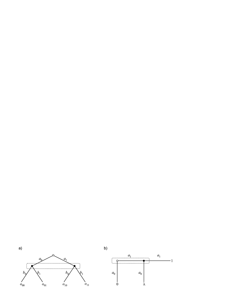
Figure 1: Examples of decision problems with imperfect recall.

As we have mentioned in preliminaries, the decision maker has two different ways to precise her decision - expressed as mixed strategies or as behavioral strategies. Her set of pure strategies is $\{a_{0}b_{0},a_{0}b_{1},a_{1}b_{0},a_{1}b_{1}\}$ where the first (second) entry of $a_{k}b_{l}$ means an action taken by the decision maker when she is in the first (second) information set. Thus, she can choose mixed strategy as a probability distribution over $a_{k}b_{l}$. On the other hand the decision maker can specify an independent probability measure over actions available at each information set i.e., her behavioral strategy is of the form $((p,1-p),(q,1-q))$. This example shows no outcome-equivalence between mixed and behavioral strategies. To be precise, there are outcomes induced by some mixed strategies that are not achievable by any behavioral strategy. To see this, let us consider an outcome of the form $p_{1}o_{00}+(1-p_{1})o_{11}$, $p\in(0,1)$. This outcome is obtained from a mixed strategy $(p_{1},0,0,1-p_{1})$. However, no behavioral strategy can yield this outcome. To see this, notice that any behavioral strategy $((p,1-p),(q,1-q))$ must assign probability $p(1-q)$ equal 0 to yield the outcome $p_{1}o_{00}+(1-p_{1})o_{11}$. It implies that the probability of obtaining either $o_{00}$ or $o_{11}$ is equal 0.
Let us take a look how the EWL scheme can be applied to the problem described above. Looking at the game tree we can see that this problem has the same structure as an extensive form of a $2\times 2$ strategic game. The decision maker before making her first move takes on the role of the player 1 and afterwards takes an action available for the player 2. As she has forgotten the action taken previously, she has the same knowledge of the game as players in $2\times 2$ game. It is therefore natural to adapt to this problem the EWL scheme when the decision maker chooses some unitary operator $U_{1}$ with which she acts on the first qubit $|\varphi\rangle_{1}$ and subsequently applies a unitary operator $U_{2}$ on the second qubit $|\varphi\rangle_{2}$. Then a payoff is calculated through the formula (3). The formal description of this problem in a manner comparable to (4) is as follows:

$$H^{\prime}=\{\emptyset,U_{1}|\varphi\rangle_{1},(U_{1}|\varphi\rangle_{1},U_{2}|\varphi\rangle_{2})\};$$

$$u^{\prime}=\mathrm{E}(O)(U_{1}\otimes U_{2}),~{}~{}I^{\prime}=\{\{|\varphi\rangle_{1}\},\{|\varphi\rangle_{2}\}\}.$$ (5)

It should be emphasized that we do not try to identify each component from Definition 2.1 with components of (5). Specification (5) takes on the informal character. It is aimed at organizing our deliberations. The main feature of the EWL scheme is that it comprises corresponding classical game i.e., there exists a set of unitary operators that yield the same outcomes as classical strategies. That is, classical actions can be realized via $I$ and $i\sigma_{x}$ as it has been shown, for example, in [9]. The decision maker’s strategies are not single actions in the problem (5), however. They are plans that describe what does the decision maker do in each of her two information sets (see Definition 2.2), i.e., what unitary action she performs on each of two qubits individually. Therefore, her set of pure classical strategies can be described as $\{I\otimes I,I\otimes i\sigma_{x},i\sigma_{x}\otimes I,i\sigma_{x}\otimes i\sigma_{x}\}$. Then a classical mixed strategy can be obtained by

$$\sqrt{p_{1}}I\otimes I+\sqrt{p_{2}}I\otimes i\sigma_{x}+\sqrt{p_{3}}i\sigma_{x}\otimes I+\sqrt{p_{4}}i\sigma_{x}\otimes i\sigma_{x}$$ (6)

where $|\sqrt{p_{i}}|^{2}$ are the values of some probability mass function (notice that $\sqrt{p_{i}}$ can take complex values). In general case a (pure) unitary strategy takes the form $U_{1}(\theta_{1},\alpha_{1},\beta_{1})\otimes U_{2}(\theta_{2},\alpha_{2},\beta_{2})$. In games represented by bimatrices the equivalence (with respect to outcomes that can be achieved) between classical actions and some fixed unitary operators is sufficient to claim that a quantum realization generalizes the classical game. In extensive games, particularly in the decision problem (5), it seems natural to find unitary strategies that realize classical behavioral strategies, not only mixed strategies. Following [9], we know that a unitary strategy $U_{1}(\theta_{1},0,0)\otimes U_{2}(\theta_{2},0,0)$ must imitate some classical move of the decision maker. This strategy corresponds exactly to classical behavioral strategy $((p,1-p),(q,1-q))$. If we assume $p\equiv\cos^{2}(\theta_{1}/2)$ and $q\equiv\cos^{2}(\theta_{1}/2)$, we obtain from (3):

$$\mathrm{E}(O)(\theta_{1},\theta_{2})=\sum_{k,l\in\{0,1\}}o_{kl}\cos^{2}\left(\frac{\theta_{1}-k\pi}{2}\right)\cos^{2}\left(\frac{\theta_{2}-l\pi}{2}\right).$$ (7)

Since one-parameter operators $U_{j}(\theta_{j},0,0)$ implement classical moves, a natural question arises: what is the role of wider range of unitary strategies in the decision problem (5)? The answer to this question is surprising: Extension of the set of behavioral strategies to the set $\mathsf{SU}(2)\otimes\mathsf{SU}(2)$ causes outcome-equivalence of behavioral strategies with mixed strategies. Notice that this problem is not trivial because there is no identity of the expression (6) and $U_{1}(\theta_{1},\alpha_{1},\beta_{1})\otimes U_{2}(\theta_{2},\alpha_{2},\beta_{2})$. For example, if one puts $\sqrt{p_{1}}=\sqrt{p_{4}}=\frac{1}{\sqrt{2}}$ and $\sqrt{p_{2}}=\sqrt{p_{3}}=0$, there is no representation of (6) in the form of the tensor product of (2). On the other hand when we take, for example, $\alpha_{1}=\alpha_{2}\neq 0$ then the tensor product $U_{1}(\theta_{1},\alpha_{1},\beta_{1})\otimes U_{2}(\theta_{2},\alpha_{2},\beta_{2})$ has not the form of a mixed strategy for any angles $\theta_{1},\theta_{2},\beta_{1},\beta_{2}$. However, the following statement is true:

Proposition 4.1

For any mixed strategy of a decision maker in the decision problem (5) there is an outcome-equivalent pure unitary strategy.

Proof. The set of outcomes yielded by all mixed strategies is a convex hull of elements $\{o_{00},o_{01},o_{10},o_{11}\}$ due to the expression for a mixed strategy (6) or, equivalently, a mixed strategy of the decision problem (4). We will prove that any convex combination $\sum_{k,l\in\{0,1\}}p_{kl}o_{kl}$ can be written as an expected outcome $\mathrm{E}(O)(U_{1}\otimes U_{2})=\sum_{k,l\in\{0,1\}}o_{kl}|\langle\psi_{f}|kl\rangle|^{2}$ for some unitary operations $U_{1}$ and $U_{2}$ from $\mathsf{SU}(2)$. At first let us consider the case $p_{00}=p_{11}=0$ or $p_{01}=p_{10}=0$. Then the convex combination $\sum_{k,l\in\{0,1\}}p_{kl}o_{kl}$ is a segment $p_{01}o_{01}+p_{10}o_{10}$ or $p_{00}o_{00}+p_{11}o_{11}$, respectively. Putting $U_{1}(0,\alpha_{1},0)\otimes U_{2}(0,0,0)$ we get $\mathrm{E}(O)=o_{00}\cos^{2}\alpha_{1}+o_{11}\sin^{2}\alpha_{1}$ that is a segment linking points $o_{00}$ and $o_{11}$. Similarly, if we take $U_{1}(\pi,0,\beta_{1})\otimes U_{2}(0,0,0)$ we obtain $o_{01}\sin^{2}\beta_{1}+o_{10}\cos^{2}\beta_{1}$. Now, let us examine general convex combination of points $o_{kl}$ such that $p_{00}+p_{11}\neq 0$ and $p_{01}+p_{10}\neq 0$. The combination $\mathrm{E}(O)$ associated with $U_{1}(\theta_{1},\alpha_{1},\beta_{1})\otimes U_{2}(0,0,0)$ is of the form:

$$\left(o_{00}\cos^{2}\alpha_{1}+o_{11}\sin^{2}\alpha_{1}\right)\cos^{2}\frac{\theta_{1}}{2}+\left(o_{01}\sin^{2}\beta_{1}+o_{10}\cos^{2}\beta_{1}\right)\sin^{2}\frac{\theta_{1}}{2}.$$ (8)

Comparing the coefficients of the combination $\sum_{k,l\in\{0,1\}}p_{kl}o_{kl}$ and (8) we obtain the system of equations that has a unique solution:

$$\cos^{2}\frac{\theta_{1}}{2}=p_{00}+p_{11},~{}~{}\cos^{2}\alpha_{1}=\frac{p_{00}}{p_{00}+p_{11}},~{}~{}\cos^{2}\beta_{1}=\frac{p_{10}}{p_{01}+p_{10}}.$$ (9)

The result (9), together with the first case, finishes the proof. $\blacksquare$

Notice that the unitary strategies used in the proof depend only on an operation on the first qubit. Due to the fact that the qubits are maximally entangled every outcome can be obtained by performing an operation only on the first or only on the second qubit.

4.2 Application 2

The next example in which we are going to use the EWL scheme is based on [3]. As the previous example, this one also shows difference between reasoning based on mixed and behavioral strategies. The application is dealing with the well-known imperfect recall problem called the paradox of absentminded driver. Our research is not the first attempt to put this problem into quantum domain. The first one appeared in [11]. The authors of this paper presented the way of quantization with the use of the Marinatto and Weber scheme of playing quantum $2\times 2$ games [12] - the initial state plays the main role. In outline, for many kinds of the absentminded driver problems various initial states are chosen to maximize the driver’s payoff. Therefore, we expect that no other protocol could be ahead of [11] in terms of maximization of the driver’s payoff. However, the quantum version based on the EWL protocol turns out to be a convenient way to make an analysis of some complicated cases of the problem of absentminded driver.

4.2.1 The paradox of absentminded driver.

The name of this decision problem is derived from a certain story describing this issue. An individual sitting for some time in a pub eventually decides to go back home. The way is leading through the motorway with two subsequent exits. The first exit leads to a catastrophic area (payoff 0). The choice of the other one will lead the decision maker home (payoff $\lambda>2$). If he continues his journey along the motorway not choosing any of the exits, he will not be able to go back home but he has a possibility to stay for the night at a motor lodge (payoff 1). The key determinant is the driver’s absent-mindedness. This means that when he arrives at the exit he is not able to tell if it is the first or the second exit due to his absent-mindedness. This situation is described on Figure 1b. The formal description is as follows:

$$H=\{\emptyset,a_{0},a_{1},(a_{1},a_{0}),(a_{1},a_{1}),\},~{}~{}I=\{\emptyset,a_{1}\};$$

$$u(a_{0})=0,~{}~{}u(a_{1},a_{0})=\lambda,~{}~{}u(a_{1},a_{1})=1.$$ (10)

Let us determine decisions that the driver can make. Since the decision maker has just one information set, according to Definition 2.2, only two pure strategies are available to him: ‘exit’ or ‘motorway’ with respective terminal histories $a_{0}$ and $(a_{1},a_{1})$. Similarly, behavioral strategy of the driver will be represented by the same random device in each of the two nodes of the information set i.e., it is on the form $(p,1-p)$ where $p$ is the probability of choosing ‘exit’. Notice first that the driver plans his journey still sitting in the bar which is equivalent to choosing some pure strategy. The optimal strategy is ‘motorway’ (with corresponding payoff 1) which becomes paradoxical when the decision maker begins carrying out this pure strategy. It is better for him, when he approaches an exit, to go away from the motorway because he comes to a conclusion that with equal probability he is at the first or the second exit. Consequently, his optimal choice will be a certain behavioral strategy. For example if $\lambda=4$, the expected payoff corresponding to the strategy $(p,1-p)$ is expressed by $u(p,1-p)=(1-p)(1+3p)$. Maximizing $u(p,1-p)$ we conclude that the optimal decision for the decision maker is to choose ‘exit’ with probability $1/3$ each time he encounters an intersection, which corresponds to the expected payoff $4/3$. As in the previous example, here as well we can notice lack of equivalence between behavioral and mixed strategies. This time, however, behavioral strategy is strictly better than mixed one as it ensures strictly higher payoff for the driver. Observe, however, that condition $\lambda>2$ is essential for this case. Otherwise, $p=0$ maximizes the expected payoff $u(p,1-p)$ which is equal 1.

Now, we are going to implement the EWL protocol to this problem. It is possible since in the classical example we have again a decision problem with two stages. Moreover, actions are taken independently at each of these stages as in the $2\times 2$ bimatrix game. Further, each player in the $2\times 2$ game has not any knowledge of an action taken by his opponent. Therefore, this is the same situation as if the decision maker was in the role of the player 1 and then the player 2, and he forgot his previous move. Let us assign the state after each action of the classical decision problem with the computational base of respective qubit. States induced by actions: ‘exit’ and ‘motorway’ available after history $\emptyset$ correspond to $|0\rangle$ and $|1\rangle$ states of the first qubit $|\varphi\rangle_{1}$. Similarly, we assign states after actions from $A(a_{1})$ (see Definition 2.1) to base states of the second qubit $|\varphi\rangle_{2}$. Notice that this is the obvious procedure applied in quantum $2\times 2$ bimatrix games where outcomes are assigned to base states $|kl\rangle$ where $k,l\in\{0,1\}$. We assume, as in the classical case, that in the quantum realization the driver is unable to distinguish to which qubit he applies a unitary action. Therefore, the two qubits are in the information set. It implies that the same unitary operation $U$ is applied to both qubits. More formally:

$$H^{\prime}=\{\emptyset,U|\varphi\rangle_{1},(U|\varphi\rangle_{1},U|\varphi\rangle_{2})\},~{}~{}I^{\prime}=\{|\varphi\rangle_{1},|\varphi\rangle_{2}\};$$

$$\mathrm{E}(u)\left(U^{\otimes 2}\right)=\lambda|\langle\psi_{f}|10\rangle|^{2}+1|\langle\psi_{f}|11\rangle|^{2}~{}~{}\mbox{and}~{}~{}|\psi_{f}\rangle=J^{{\dagger}}U^{\otimes 2}J|00\rangle.$$ (11)

The core of the issue lies in the payoff function $\mathrm{E}(u)$. If state $|0\rangle$ on the first qubit is measured (which corresponds to choosing ‘exit’ at the first intersection), the payoff assigned to this state equals 0 regardless of the state measured on the second qubit. Therefore, in (11) the expected payoff $\mathrm{E}(u)$ includes $0\left(|\langle\psi_{f}|00\rangle|^{2}+|\langle\psi_{f}|01\rangle|^{2}\right)$. Thus, so defined quantum realization generalizes the classical case. The classical pure strategies can be again implemented by $I$ and $i\sigma_{x}$ which correspond to ‘exit’ and ‘motorway’, respectively. These strategies imply operations $I^{\otimes 2}$ and $(i\sigma_{x})^{\otimes 2}$ on both qubits that are indistinguishable by the decision maker, and produce outcomes equal to classical ones. Although we have assumed that the result 0 on the first qubit determine payoff 0, we always have to specify operations on both qubits. Like in the classical case, also here decision maker’s strategy have to precise an action in every possible state of a decision problem. As in the previous example one-parameter operation $U(\theta,0,0)$ matches classical behavioral strategy and we have:

$$\mathrm{E}(u)(\theta)=\lambda\sin^{2}\frac{\theta}{2}\cos^{2}\frac{\theta}{2}+1\sin^{4}\frac{\theta}{2}.$$ (12)

If we replace $\cos^{2}(\theta/2)$ by $p$ in the formula (12) we obtain expected payoff that corresponds to the classical behavioral strategy $(p,1-p)$ in the decision problem (10). From the classical case (10) we already know that the driver can obtain the maximal payoff which is $4/3$ when $\lambda=4$, using operators of the type $U(\theta,0,0)$. Let us investigate if the decision maker can benefit when the range of his actions is extended to any operator of the form (2). Assume that the driver has two-parameter set of unitary operations $U(\theta,\alpha,0)$ at his disposal. Then the expected payoff is as follows:

$$\mathrm{E}(u)(\theta,\alpha)=\frac{1}{4}\lambda(\sin 2\alpha+1)\sin\theta+\left(\sin(2\alpha)\cos^{2}\frac{\theta}{2}-\sin^{2}\frac{\theta}{2}\right)^{2}$$ (13)

If the driver applies $U(\pi/2,\pi/4,0)$ to his both qubits, the expected payoff equals $\lambda/2$. Coming back to the case $\lambda=4$, he gets 2 utilities instead of $4/3$. Moreover, this is the highest payoff which the driver can guarantee himself by using any unitary operations (2). To prove this, we determine the final state $|\psi_{f}\rangle$ when any unitary operation $U(\theta,\alpha,\beta)^{\otimes 2}$ is given. The matrix representation of $|\psi_{f}\rangle$ takes the form:

$$|\psi_{f}\rangle=\left(\begin{array}[]{c}\displaystyle\cos 2\alpha\cos^{2}\frac{\theta}{2}+\sin 2\beta\sin^{2}\frac{\theta}{2}\\ \displaystyle i\left(\cos\frac{\theta}{2}\sin\frac{\theta}{2}(\cos(\alpha-\beta)+\sin(\alpha-\beta)\right)\\ \displaystyle i\left(\cos\frac{\theta}{2}\sin\frac{\theta}{2}(\cos(\alpha-\beta)+\sin(\alpha-\beta)\right)\\ \displaystyle\sin 2\alpha\cos^{2}\frac{\theta}{2}-\cos 2\beta\sin^{2}\frac{\theta}{2}\end{array}\right).$$ (18)

Therefore, the state $|\psi_{f}\rangle$ is a particular case of the state $|\psi^{\prime}_{f}\rangle$ of the form:

$$|\psi^{\prime}_{f}\rangle=\sum_{k,l\in\{0,1\}}\eta_{kl}|kl\rangle,~{}\mbox{where}~{}\eta_{kl}\in\mathbb{C},\sum_{k,l\in\{0,1\}}|\eta_{kl}|^{2}=1~{}\mbox{and}~{}\eta_{01}=\eta_{10}.$$ (19)

Exchanging $|\psi_{f}\rangle$ by $|\psi^{\prime}_{f}\rangle$ in (11), we see that the expected payoff $\mathrm{E}^{\prime}(u)$ equals $\lambda|\eta_{10}|^{2}+|\eta_{11}|^{2}$. Furthermore, we have $\lambda>2$. It implies that the set $\mathrm{arg}\max_{\eta_{kl}}(\mathrm{E}^{\prime}(u))$ consists of all points $(\eta_{10},\eta_{11})$ for which $(|\eta_{10}|^{2},|\eta_{11}|^{2})=(1/2,0)$. It is obvious that in the special case $|\psi_{f}\rangle$ the equality $\mathrm{arg}\max_{\psi_{f}}(\mathrm{E}(u)(\theta,\alpha,\beta))=\mathrm{arg}\max_{\psi_{f}}(|\langle\psi_{f}|10\rangle|^{2})$ is fulfilled as well. As we obtain $\max_{\psi_{f}}(|\langle\psi_{f}|10\rangle|^{2})=1/2$, the decision maker can achieve maximal payoff equal to $\lambda/2$. Observe that the maximal payoff that the decision maker can get in the classical case is $\lambda^{2}/4(\lambda-1)$. This is strictly less than $\lambda/2$ if only $\lambda>2$. This leads us to the conclusion that in the decision problem (10) extended to the quantum domain there exists the unitary strategy for any $\lambda>2$ that is strictly better than any classical one.

4.2.2 The n-tuple paradox of absentminded driver.

We have already showed the advantage of quantum strategies over classical ones in the problem of absentminded driver. Now, we test unitary strategies in the case where the driver comes across more than one treacherous intersection. At this moment we make an assumption that the absentminded driver problem is characterized by $n+1$ intersections such that the first $n$ intersections are treacherous ones (payoff 0 when ‘exit’ is chosen at each of these intersections), and only one action ‘exit’ taken at n+1 intersection leads the driver home (payoff $\lambda$). Choosing the action ‘motorway’ all the time yields payoff 1, the same as in (10). This problem is depicted on Figure 2.

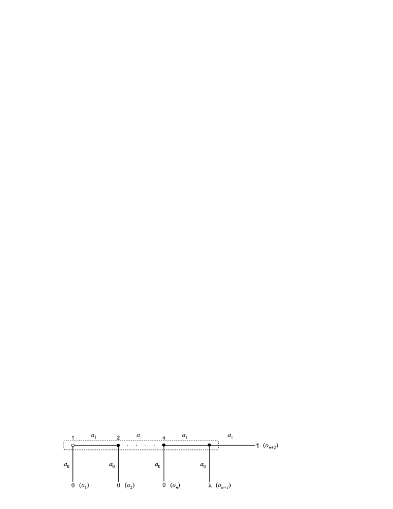
Figure 2: The n-tuple decision problem of absentminded driver.

A formal description of this classical case is similar to (10). To find an optimal classical strategy we have to maximize $(1-p)^{n}((\lambda-1)p+1)$ In quantum version we apply the general EWL protocol for $(n+1)\times(n+1)$ bimatrix game where entangling operator $J$ and final state $|\psi_{f}\rangle$ take the form given in [4]:

$$J=\frac{1}{\sqrt{2}}(I^{\otimes n+1}+i\sigma_{x}^{\otimes n+1}),~{}~{}|\psi_{f}\rangle=J^{{\dagger}}U^{\otimes n+1}J|0\rangle^{\otimes n+1}$$ (20)

The decision maker carries out some fixed unitary operation $U\in\mathsf{SU}(2)$ on each of $n+1$ qubits. In addition, the qubits belong to the same information set:

$$H^{\prime}=\{\emptyset,U|\varphi\rangle_{1},(U|\varphi\rangle_{1},U|\varphi\rangle_{2}),\dots,(U|\varphi\rangle_{1},U|\varphi\rangle_{2},\dots,U|\varphi\rangle_{n+1})\};$$

$$I^{\prime}=\{|\varphi\rangle_{1},|\varphi\rangle_{2},\dots,|\varphi\rangle_{n+1}\};$$

$$\mathrm{E}(u)\left(U^{\otimes n+1}\right)=\lambda|\langle\psi_{f}|1\rangle^{\otimes n}|0\rangle|^{2}+|\langle\psi_{f}|1\rangle^{\otimes n+1}|^{2}.$$ (21)

We identify the states after actions ‘exit’ and ‘motorway’ of the decision problem from Figure 2 with states $|0\rangle$ and $|1\rangle$, respectively, exactly like in (11). This causes the equivalence between the decision problem (21) with unitary operators reduced to one-parameter operators $U(\theta,0,0)$ and the classical case, in the same way as in (10) and (11):

$$\mathrm{E}(\theta)=\lambda\cos^{2}\frac{\theta}{2}\sin^{2n}\frac{\theta}{2}+\sin^{2(n+1)}\frac{\theta}{2}.$$ (22)

The $n$ payoffs equal 0 could suggest these ones are essential so that the EWL scheme can generalize the decision problem depicted in Figure 2, but this is not true. In fact, any decision problem given by the decision tree depicted in Figure 2 can be implemented by the EWL scheme. (Notice that (10) represents any decision problem given by the decision tree shown in Figure 1b as it comes down to a problem with payoffs $0,\lambda,1$ through adding a respective constant to all the payoffs and (or) multiplying all the payoffs by a respective constant). To demonstrate that the EWL quantum representation defines correctly any kind of the n-tuple paradox, we assign, instead of fixed payoffs, outcomes $o_{1},o_{2},\dots,o_{n+2}$ to the terminal histories. Then the n-tuple decision problem takes the form:

$$H^{\prime}=\{\emptyset,a_{0},a_{1},\dots,(a^{1}_{1},\dots,a^{n}_{1},a^{n+1}_{0}),(a^{1}_{1},\dots,a^{n}_{1},a^{n+1}_{1})\};$$

$$I^{\prime}=\{\emptyset,a_{1},\dots,(a^{1}_{1},\dots,a^{n}_{1},a^{n+1}_{1})\};$$

$$O(a_{0})=o_{1},~{}~{}O(a^{1}_{1},\dots,a^{t}_{1},a^{t+1}_{0})=o_{t+1}~{}~{}\mbox{for}~{}~{}t=1,2,\dots,n.$$ (23)

Let us denote by $|j_{1},j_{2},\dots,j_{n+1}\rangle\in\bigotimes_{n+1}\mathbb{C}^{2}$ an element of the computational base. For any $t=1,2,\dots,n$ a symbol $(j_{t},j_{t+1},\dots,j_{n+1})_{2}$ denotes the binary representation of a (decimal) number .

Proposition 4.2

The decision problem (21) with unitary operators $U$ restricted to $U(\theta,0,0)$ and expected payoff function $\mathrm{E}(O)$ extended to include:

$$\sum_{t=1}^{n}o_{t}\sum_{x=0}^{2^{n-t+1}-1}|\langle\psi_{f}|1\rangle^{\otimes t-1}|0\rangle|x\rangle|^{2}~{}~{}\mbox{where}~{}~{}x=(j_{t+1},j_{t+2},\dots,j_{n+1})_{2}$$ (24)

implements the decision problem (23).

Proof. First we calculate $U(\theta,0,0)^{\otimes n+1}J|0\rangle^{\otimes n+1}$ where $J$ is defined by (20). Then the expression $\sqrt{2}U^{\otimes n+1}J|0\rangle^{\otimes n+1}$ takes the form:

$$\sum_{y=0}^{2^{n+1}-1}\left(i^{r(y)}\cos^{n-r(y)+1}\frac{\theta}{2}\sin^{r(y)}\frac{\theta}{2}-i^{n-r(y)}\cos^{r(y)}\frac{\theta}{2}\sin^{n-r(y)+1}\frac{\theta}{2}\right)|y\rangle$$ (25)

where the element $r(y)$ depends on $y=(j_{1},j_{2},\dots,j_{n+1})_{2}$ and is given be the formula $r(y)=j_{1}+j_{2}+\dots+j_{n+1}$. Let us fix any element $|y\rangle$ from the computational base and determine the inner product $\langle y|\psi_{f}\rangle$. To avoid laborious computation that are necessary to obtain complete form of the final state $|\psi_{f}\rangle$ we can choose the following simpler way to calculate the inner product. We take the bra vector $J^{{\dagger}}_{y,\cdot}=(\langle y|-i\langle\overline{y}|)\sqrt{2}$ where $|\overline{y}\rangle=\sigma_{x}^{\otimes n+1}|y\rangle$. In a language of matrices the element $J^{{\dagger}}_{y,\cdot}$ is the $y$-th row of a matrix representation of $J^{{\dagger}}$. Next, let us put $P$ as a label of a projector $|y\rangle\langle y|+|\overline{y}\rangle\langle\overline{y}|$. Then $\langle y|\psi_{f}\rangle$ can be expressed as follows:

$$\langle y|\psi_{f}\rangle=J^{{\dagger}}_{y,\cdot}PU^{\otimes n+1}J|0\rangle^{\otimes n+1}.$$ (26)

Notice that $r(y)$ and $r(\overline{y})$ are connected through equation $r(y)+r(\overline{y})=n+1$. Using this fact and a result from (25) the amplitude associated with $|\overline{y}\rangle$ of the state $U^{\otimes n+1}J|0\rangle^{\otimes n+1}$ is given by

$$\frac{1}{\sqrt{2}}\left(i^{r(\overline{y})}\cos^{r(y)}\frac{\theta}{2}\sin^{r(\overline{y})}\frac{\theta}{2}-i^{n-r(\overline{y})}\cos^{r(\overline{y})}\frac{\theta}{2}\sin^{r(y)}\frac{\theta}{2}\right).$$ (27)

In order to complete the state $PU^{\otimes n+1}J|0\rangle^{\otimes n+1}$ we just copy the amplitude of $|y\rangle$ from (25). If we use (26) and (27) we will receive the final form of $\langle y|\psi_{f}\rangle$:

$$\langle y|\psi_{f}\rangle=i^{r(y)}\cos^{r(\overline{y})}\frac{\theta}{2}\sin^{r(y)}\frac{\theta}{2}.$$ (28)

The result (28) together with substitution $p=\cos^{2}(\theta/2)$ immediately gives us $|\langle\psi_{f}|y\rangle|^{2}=p^{r(\overline{y})}(1-p)^{r(y)}$. After some calculations we conclude from the last result that:

$$\sum_{x}|\langle\psi_{f}|y\rangle|x\rangle|^{2}=p^{r(\overline{y})}(1-p)^{r(y)}\sum_{x}{r(x)+r(\overline{x})\choose r(x)}p^{r(\overline{x})}(1-p)^{r(x)}$$ (29)

The sum on the right-hand side of the equation (29) is the Newton s formula which is equal 1. Therefore, the formula (29) leads us to a conclusion that for any $t=1,2,\dots,n$ the component assigned to $o_{t}$ of the formula (24) can be expressed as:

$$\sum_{x}|\langle\psi_{f}|1\rangle^{\otimes t-1}|0\rangle|x\rangle|^{2}=(1-p)^{t-1}p.$$ (30)

Equation (30) ends the proof as the right-hand side of the equation is a probability of the outcome $o_{t}$ in the decision problem (23) when a behavioral strategy $(p,1-p)$ is taken. $\blacksquare$

It follows from Proposition 4.2 that every time when we concern the classical problem depicted on Figure 2 we can consider the problem (21) when unitary operators (2) are restricted to one-parameter operators $U(\theta,0,0)$ and the payoff function is given by (22).

Let us return to example (21) where a payoff function is fixed. Let us check if unitary operators (2) can yield strictly better results than any classical strategies applied to the problem. In order to do that, we need to determine the expected payoff $\mathrm{E}(u)(U)$ defined in (21) for any $U(\theta,\alpha,\beta)\in\mathsf{SU}(2)$ . We can find the components $|\langle\psi_{f}|1\rangle^{\otimes n}|0\rangle|^{2}$ and $|\langle\psi_{f}|1\rangle^{\otimes n+1}|^{2}$ of $\mathrm{E}(u)(U)$ with the use of equation (26). After simple calculations we get:

$$\mathrm{E}(u)(U) = \lambda|i\cos^{n}\frac{\theta}{2}\sin\frac{\theta}{2}\sin(n\alpha-\beta)+i^{n}\cos\frac{\theta}{2}\sin^{n}\frac{\theta}{2}\cos(\alpha-n\beta)|^{2}$$ (31)

$$+ 1|\cos^{n+1}\frac{\theta}{2}\sin[(n+1)\alpha]+i^{n+1}\sin^{n+1}\frac{\theta}{2}\cos[(n+1)\beta]|^{2}.$$

Comparing the payoffs (22) and (31) we really ought to expect better results yielded by 3-parameter operators.

Example 4.3

For $n=3$ and $\lambda=20$ the maximization result of (22) and (31) is as follows:

$$\mbox{classical scenario:}~{}~{}\max_{\theta}{\mathrm{E}(u)(\theta)}\approx\mathrm{E}(u)\left(\frac{7\pi}{10}\right)\approx 2,46;$$

$$\mbox{EWL scenario:}~{}~{}\max_{\theta,\alpha,\beta}{\mathrm{E}(u)(\theta,\alpha,\beta)}=\mathrm{E}(u)\left(\frac{\pi}{2},\frac{9\pi}{16},\frac{3\pi}{16}\right)=5.$$

This example shows that an increased number of treacherous intersections does not reduce the ability of the EWL scheme to yield benefit to the decision maker. Moreover, the ratio $\max_{\theta,\alpha,\beta}\mathrm{E}(u)(\theta,\alpha,\beta):\max_{\theta}\mathrm{E}(u)(\theta)$ grows together with $\lambda$. For large $n$ we had better use some mathematical software to determine the precise result of optimization. Following proposition assure us that the attempt of finding optimal solution makes sense for any $n$:

Proposition 4.4

For any $n\geqslant 1$ in the n-tuple decision problem (21) there exist a number $\lambda_{0}>1$, angles: $\theta^{\prime}\in(0,\pi)$ and $\alpha^{\prime},\beta^{\prime}\in(0,2\pi)$ such that for any payoff $\lambda^{\prime}>\lambda_{0}$ the unitary strategy $U(\theta^{\prime},\alpha^{\prime},\beta^{\prime})$ yields a payoff strictly higher than a payoff achieved by any classical strategy.

Proof. We showed in subsection 4.2.1 the case when $n=1$. So we now assume $n\geqslant 2$. Let us take the decision problem (21). For any $n\geqslant 2$ let us put $\lambda_{0}=(\cos^{2n}\frac{\theta^{\prime}}{2}\sin^{2}\frac{\theta^{\prime}}{2})^{-1}$ and unitary operator $U^{*}(\theta^{\prime},\alpha^{\prime},\beta^{\prime})$ defined by:

$$\theta^{\prime}=2\arccos\frac{1}{\sqrt{n+1}},~{}~{}\alpha^{\prime}=\frac{(\pi+2\pi\chi_{A}(n))n}{2(n^{2}-1)},~{}~{}\beta^{\prime}=\frac{\pi+2\pi\chi_{A}(n)}{2(n^{2}-1)}.$$ (32)

where $\chi_{A}(n)$ is an indicator function of a set $A=\{n\colon i^{n-1}=-1\}$. Notice that $\lambda_{0},\theta^{\prime},\alpha^{\prime}$ and $\beta^{\prime}$ all meet the requirements of the proposition. They depend only on $n$. Further, $\lambda_{0}$ is well defined as $\theta^{\prime}\notin\{0,\pi\}$. For any $\delta>1$ let us denote $\lambda^{\prime}=\delta\lambda_{0}$ the payoff associated with the problem (21). By putting parameters (32) into formula (31) and comparing it to (22), and by using the fact that $\theta^{\prime}\in\mathrm{arg\,max}_{\theta}\left(\cos^{2}\frac{\theta}{2}\sin^{2n}\frac{\theta}{2}\right)$, we obtain the following sequence of inequalities:

$$\mathrm{E}(u)(U^{*}) \geqslant \lambda^{\prime}\left(\cos^{2n}\frac{\theta^{\prime}}{2}\sin^{2}\frac{\theta^{\prime}}{2}+\cos^{2}\frac{\theta^{\prime}}{2}\sin^{2n}\frac{\theta^{\prime}}{2}\right)=\delta+\lambda^{\prime}\cos^{2}\frac{\theta^{\prime}}{2}\sin^{2n}\frac{\theta^{\prime}}{2}$$ (33)

$$> 1+\lambda^{\prime}\cos^{2}\frac{\theta^{\prime}}{2}\sin^{2n}\frac{\theta^{\prime}}{2}\geqslant\max_{\theta\in[0,\pi]}\mathrm{E}(u)(\theta),$$

which completes the proof. $\blacksquare$

Let us observe now, how Proposition 4.4 concerns the result of quantization the absentminded driver in subsection 4.2.1. A segment of numbers $\lambda$ in which there exists unitary strategy strictly better than classical one, is the segment $(2,\infty)$. It can be easily proved that for any $\lambda\in\mathbb{R}\setminus(2,\infty)$ the maximal payoff of the decision problem (10) is equal 1 regardless of used unitary strategies. Proposition 4.4 shows that the problem of finding optimal unitary strategy in decision problems with various numbers of the treacherous intersections is very much alike.

5 Conclusion

We have found the new use of the EWL protocol beyond strategic $2\times 2$ games. It turns out once again that game theory defined on quantum domain provides results that are inaccessible in classical game theory. We have confirmed through Proposition 4.4 that we can increase maximal payoff in decision problems carried out via the EWL scheme. Our research has allowed to formulate Proposition 4.1 that points out another peculiarity of quantum games. Unitary strategies (2) that include classical behavioral ones (when they are restricted to one-parameter operators) can be outcome equivalent to unitary operators implementing classical mixed strategies while behavioral and mixed strategies are not outcome equivalent in classical decision problems. These surprising features make quantum games worth further thorough studies.

References

• [1] J. Eisert, M. Wilkens and M. Lewenstein (1999), Quantum games and quantum strategies, Phys. Rev. Lett. 83, 3077-3080.
• [2] M.Β J. Osborne and A. Rubinstein (1994), A Course in Game Theory, MIT Press.
• [3] M. Piccione and A. Rubinstein (1997), On the interpretation of decision problems with imperfect recall, Games and Economic Behavior 20, 3-24.
• [4] S.C. Benjamin and P.M. Hayden (2001), Multiplayer quantum games, Phys. Rev. A 64, 030301.
• [5] R. B. Myerson (1991), Game Theory: Analysis of Conflict, Harvard University Press.
• [6] A. Nawaz and A. H. Toor (2006), Quantum games with correlated noise, J. Phys. A: Math. Gen. 39 9321.
• [7] A. P. Flitney and D. Abbott (2003), Advantage of a quantum player over a classical one in $2\times 2$ quantum games, Proc. R. Soc. Lond. A, 459, 2463-2474.
• [8] A. P. Flitney and L. C. L Hollenberg (2007), Nash equilibria in quantum games with generalized two-parameter strategies, Phys. Lett. A 363, 381-388.
• [9] J. Eisert and M.Wilkens (2000), Quantum games, J. Mod. Opt. 47 2543.
• [10] J. Du, H. Li, X. Xu, X. Zhou and R. Han (2002), Entanglement enhanced multiplayer quantum games, Phys. Lett. A 302, 229-233.
• [11] A. Cabello and J. Calsamiglia (2005), Quantum entanglement, indistinguishability, and the absent-minded driver’s problem, Physics Letters A 336 441-447
• [12] L. Marinatto and T. Weber (2000), A quantum approach to static games of complete information, Phys. Lett. A 272, 291-303.