Diffusion and Multiplication in Random Media

Abstract

We investigate the evolution of a population of non-interacting particles which undergo diffusion and multiplication. Diffusion is assumed to be homogeneous, while multiplication proceeds with different rates reflecting the distribution of nutrients. We focus on the situation where the distribution of nutrients is a stationary quenched random variable, and show that the population exhibits a super-exponential growth whenever the nutrient distribution is unbounded. We elucidate a huge difference between the average and typical asymptotic growths and emphasize the role played by the spatial correlations in the nutrient distribution.

I Introduction

The evolution of a population in an inhomogeneous environment with spatially varying growth rates can display complex dynamical patterns, resulting from the competition between diffusion, random multiplication and possibly advection Zeldovich ; ran_medium . Inhomogeneities of the environment can greatly affect the population dynamics resulting in anomalous spreading (neither diffusive, nor ballistic) and intermittent behaviors (for a review on intermittency in random media see, e.g., Zeldovichreview ) with patches of population growing in favorable places and being surrounded by large desertic regions. Diffusion tails play the role of vanguard agents that explore hostile regions, in search of ever-more hospitable locations to settle and to multiply. The offspring in the new settlement will eventually outgrow the original colony and generate a strong gradient current: this can be seen as a migration of the whole population. A simple and concrete example of this problem is provided by bacteria multiplying and diffusing in a petri dish where nutrients and inhibitors are unevenly distributed, resulting in complex growth patterns that are observable in actual experiments Murray ; Budrene . In a more abstract setting, the actual inhomogeneous space can be replaced by a rough phenotypic landscape in which the fitness functional (that governs the growth rate) takes different values: here the coordinate variable does not label a spatial location but rather the genetic content of each individual. This point of view has been inspired by S. Wright, R. A. Fisher and J. B. S. Haldane’s classical studies in population genetic Ewens . More recently it was developed by M. Eigen Eigen as a model for punctuated evolution of quasi-species and has been further investigated by W. Ebeling et al. Ebeling , Y.-C. Zhang Zhang , M. N. Rosenbluth R and many other authors; see Baake ; Krug for a review of more recent work.

In the present work, we examine a population of non-interacting particles that diffuse and undergo the birth/death process depending on the availability of nutrients. The population density $n({\bf x},t)$ evolves according to the diffusion equation with a multiplicative noise:

$$\frac{\partial n({\bf x},t)}{\partial t}=D\nabla^{2}n({\bf x},t)+\eta({\bf x})n({\bf x},t)\qquad\text{with}\qquad n({\bf x},0)=n_{0}({\bf x}).$$ (1)

The diffusion coefficient $D$ is assumed to be uniform, while the birth/death rate $\eta({\bf x})$ is inhomogeneous. We shall focus on the simplest case of the stationary noise, $\eta=\eta({\bf x})$, and investigate how spatial correlations of the noise affect the growth rate of $n({\bf x},t)$.

The Langevin equation (1) is linear, reflecting the basic assumption that particles do not interact. The noise $\eta({\bf x})$ is known through its stochastic properties and changing these properties may drastically affect the behavior of $n({\bf x},t)$. Equation (1) can be generalized in various ways, e.g. one can take into account advection Nelson1 ; Nelson2 ; Nelson3 ; Schnerb , study the evolution of a vector field in a random background (e.g. a magnetic field in the dynamo effect) ran_medium , or consider several coupled fields as in the case of chemotaxis DeGennes ; Verga . One can introduce a non-linearity in order to take into account saturation effects ZeldPNAS . Besides, it can also be interesting to consider situations with $\eta=\eta({\bf x},t)$, the dependence on time reflecting e.g. seasonal variations.

Although we shall chiefly employ a population dynamics vocabulary (particles, nutrients, migrations), it is useful to keep in mind that the stochastic partial differential equation (1) arises in many different contexts. In chemical physics, reaction kinetics is often modeled by equations similar to Eq. (1) and these equations allow to predict macroscopic patterns in the spatial distribution of reagents Mikhailov1 ; Mikhailov2 . When the amplification rate $\eta(x)$ takes only negative values, equation (1) describes non-interacting particles that diffuse in a medium with random absorption. In the extreme case of $\eta(x)=-\sum_{i}\delta(x-x_{i})$ with random positions $x_{i}$ of the traps, the trapping sites become perfect because $n(x,t)$ has to vanish for $x=x_{i}$. (More precisely, the above formulation applies in one dimension; in higher dimensions, the traps should be finite and absorbing conditions are set on the boundaries of the traps.) The literature on this classical subject is vast; one of the most celebrated results asserts that the density decreases according to a stretched exponential law: $\ln n\sim-t^{d/(d+2)}$ in $d$ dimensions Varadhan ; Balagurov ; Grassberger ; Redner ; Anlauf ; Theo ; JMLTheo ; JMLlivre .

Another important interpretation of equation (1) in terms of polymer dynamics can be obtained from its formal solution,

$$n({\bf x},t)=\int d{\bf y}K({\bf x},t;{\bf y},0)\,n_{0}({\bf y})\,,$$ (2)

where the Green function $K({\bf x},t;{\bf y},0)$ is given by the Feynman-Kac formula Schulman

$$K({\bf x},t;{\bf y},0)={\bf E_{y\to x}}\left(\!\exp\left[\int^{t}_{0}\eta({\bf x}(\tau))d\tau\right]\right).$$ (3)

The expectation value ${\bf E_{y\to x}}$ with respect to the Wiener measure is taken over all paths ${\bf x}(\tau)$ that begin at ${\bf y}$ at $t=0$ and end at ${\bf x}$ at time $t$. This formula can be rewritten in more familiar manner as a path integral

$$K({\bf x},t;{\bf y},0)=\int_{{\bf x}(0)={\bf y}}^{{\bf x}(t)={\bf x}}\mathcal{D}{\bf x}(\tau)\,\exp\!\left\{\int^{t}_{0}d\tau\left[-\frac{\dot{\bf x}^{2}(\tau)}{4D}+\eta({\bf x}(\tau))\right]\right\}.$$ (4)

It is then natural to interpret ${\bf x}(\tau)$ as a $d$-dimensional Gaussian polymer in the random potential $\eta({\bf x})$ Huse ; Edwards ; Cates ; NR , or as a $d+1$-dimensional directed polymer with columnar disorder KrugHH (for a review on directed polymers see HHZ ). The physics of directed polymers in a random medium is closely related to the growth of random surfaces. In one dimension, for instance, we write $n=e^{m}$ and recast (1) into $m_{t}=D(m_{x}^{2}+m_{xx})+\eta(x)$. Differentiating this equation with respect to $x$ and writing $h=-2Dm_{x}$ we obtain

$$h_{t}+hh_{x}=Dh_{xx}+\xi(x)\,\,\hbox{ where }\,\,\xi=-2D\eta_{x}\,.$$ (5)

Thus after the transformation the noise becomes additive, but the governing Eq. (5) is now a non-linear stochastic partial differential equation. The Langevin equation (5) formally resembles the Kardar-Parisi-Zhang (KPZ) equation HHZ ; KPZ , yet the noise $\xi$ in equation (5) is stationary, whereas in the KPZ equation the noise depends both on space and time. [In the KPZ equation, the noise is typically taken to be the Gaussian white noise, $\langle\eta_{\rm KPZ}({\bf x},t)\eta_{\rm KPZ}({\bf x}^{\prime},t^{\prime})\rangle=2\Gamma\,\delta({\bf x}-{\bf x}^{\prime})\,\delta(t-t^{\prime})$.] Hence the physical properties of the solutions to Eq. (5) are significantly different from those of the standard KPZ equation Cates .

Equation (1) can also be viewed as a Schrödinger equation in imaginary time and with a random potential; it is thus related to the physics of localization JMLlivre ; Lifshitz . In the present study $n(x,t)$ is a density of particles (not a wave-function). For instance, in the no-noise case the total mass $\int dx\,n(x,t)$ is conserved, whereas the analogous integral in the quantum case is not conserved. Furthermore, we are not directly interested in eigenstates of (1) but rather in the temporal behavior of its solution starting from a localized initial state. All these differences explain why the phenomenology is rather different from that of localization, although some of the techniques developed to study quantum disordered systems are useful in the analysis of Eq. (1).

The behavior of solutions of the apparently simple linear Langevin equation (1) is not yet fully understood due to a number of puzzling features. One such feature is an astonishingly fast growth (and sometimes a blow up that occurs in a finite time, or even instantaneously R ). There are a few causes of these striking behaviors:

• The noise is multiplicative.

• In many simple models, the noise is unbounded. Hence, the regions with large positive $\eta$ play a dominant role and lead to a counter-intuitive super-exponential growth. In this situation, the discretized (in space) versions of Eq. (1) differ drastically from the strictly continuous version.

• The lack of self-averaging which is manifested by the huge difference between average and typical behaviors.

The goal of this work is to analyze the Langevin equation (1) when the noise is strongly correlated in space. Some of our results are presented in Table 1 where we display only the scaling laws (numerical constants will be given throughout the text). The part of Table 1 describing the asymptotic growth laws for the uncorrelated Gaussian white noise summarizes previous work. The notion of “correlated” noise is of course a bit vague. The one-dimensional case is exceptional as the very natural assumption that the increments of the noise are uncorrelated leads to the correlated noise $\eta(x)$ which is essentially a trajectory of a random walk (in the lattice setting) or a Brownian motion (in a continuum setting), with $x$ playing a role to time. Table 1 presents the asymptotic growth laws corresponding to such a noise. (Our main higher-dimensional results are collected in Table 2.)

Uncorrelated	Correlated ($d=1$)
Lattice substrate	Random walk landscape
$e^{t^{2}}$ (Average, all $d$)	$e^{t^{3}}$  (Average)
$e^{t{\sqrt{\ln t}}}$ (Typical, all $d$)	$e^{t^{5/3}}$   (Typical)
Continuum substrate	Brownian landscape
$e^{t^{3}}$ ($d=1$)	$e^{t^{5}}$  (Average)
Blow up $(d\geq 2)$	$e^{t^{5/3}}$   (Typical)

Table 1: Asymptotic growth laws for some of the population dynamics (numerical factors are omitted). The noise is assumed to be Gaussian, apart from the case when the noise forms a random walk landscape, that is, the increment of the noise are bounded. (The uncorrelated bounded noise is investigated in Sect. II.2.) The results for the correlated noise in higher dimensions are discussed in Sect. III.3.

The rest of this paper is organized as follows. In Sect. II, we review the behaviors when the noise is either uncorrelated or has short range correlations. We emphasize the emergence of puzzling behaviors and explain how seemingly contradictory results scattered in the literature can be synthesized in a coherent way. In Sect. III we analyze the much less studied situation of a correlated noise and determine the growth law for the total population size in the one-dimensional setting. We then qualitatively describe the situation in higher dimensions.

II Population dynamics with short-range correlations

In this section we assume that the local growth rate $\eta({\bf x})$ is on average homogeneous. Therefore, the mean value $\mu=\langle\eta\rangle$ is constant which can be set to zero; the general case is recovered by redefining the local density: $n({\bf x},t)\to n({\bf x},t)\,e^{\mu t}$. Further, because of homogeneity, the spatial correlations of $\eta$ must be translationally invariant. The simplest assumption, customary in studies of Langevin equations, is to consider the random potential $\eta$ to be uncorrelated at different spatial locations. The fluctuating potential $\eta({\bf x})$ is thus taken to be a Gaussian white noise with zero average:

$$\langle\eta\rangle=0,\qquad\langle\eta({\bf x})\eta({\bf x}^{\prime})\rangle=2\Gamma\delta({\bf x}-{\bf x}^{\prime})\,.$$ (6)

The stochastic properties of the noise are now fully specified and equation (1) defines a well-posed problem which has been studied in numerous works Zeldovich ; Zeldovichreview ; Ebeling ; Zhang ; R ; NR ; GM ; LW ; wrong ; T ; Jaya mostly in one dimension. The conclusions of these studies, established through various methods and approximations, seemed initially contradictory. However, the issue was settled in R by an exact analytical calculation based on a minimax variational principle. In the large time limit, the dominant contributions to the population density arise from very small, rapidly growing isolated regions. Although these regions are very rare and highly improbable, they produce high density peaks that dominate the whole statistics. This has led to the following unexpected asymptotic behavior in one dimension:

$$\ln\langle n(0,t)\rangle\to\frac{\Gamma^{2}t^{3}}{12D}\,\,.$$ (7)

This super-exponential growth has been also found by estimating Brownian motion expectations LW and by a path-integral approach that has additionally allowed to calculate the pre-factors of the exponential behavior T :

$$\langle n(0,t)\rangle\to\frac{\Gamma^{2}t^{5/2}}{2(\pi D^{3})^{1/2}}\,\exp\!\left(\frac{\Gamma^{2}t^{3}}{12D}\right).$$ (8)

In higher dimensions, the behavior is even more puzzling. It has been argued R ; EPGross that in two dimensions, a divergence occurs at a finite time $t_{c}\sim D/\Gamma$; for $t>t_{c}$ the solution blows up. Further, when $d>2$, the divergence is instantaneous, i.e., equation (1) with Gaussian white noise (6) is ill-defined. These striking behaviors exhibited by the Langevin equation (1) with Gaussian noise (6) are consequences of two major properties of the noise: The Gaussian noise is both uncorrelated and unbounded. We now investigate the consequences of relaxing these assumptions.

II.1 Taming the White Noise: Lattice Regularization or Finite Short-Range Correlations

The white noise displays totally uncorrelated fluctuations at all scales. However, in the present context of a population dynamics it is natural to assume some spatial coherence in the local varying conditions and that the noise has a non-vanishing correlation length. The simplest manner to implement this model is to put the system on a lattice and to assume that the noise is uncorrelated at different lattice sites. The effective correlation length is thus equal to the lattice spacing. Mathematically, one has to solve the discrete set of equations

$$\dot{n}_{\bf j}=D\nabla^{2}n_{\bf j}+n_{\bf j}\eta_{\bf j}$$ (9)

where ${\bf j}=(j_{1},\ldots,j_{d})\in\mathbb{Z}^{d}$ if the lattice is hyper-cubic. Further, the operator $\nabla^{2}$ denotes the discrete Laplacian (e.g. in one dimension we have $\nabla^{2}n_{j}=n_{j-1}-2n_{j}+n_{j+1}$). The noise in (9) is Gaussian with the following characteristics:

$$\langle\eta\rangle=0,\qquad\langle\eta_{\bf i}\eta_{\bf j}\rangle=2\Gamma\delta_{{\bf i},{\bf j}}\,.$$ (10)

In this case, the growth is chiefly universal, it is independent of the spatial dimension (up to numerical constants) and is given by $\langle n\rangle\sim e^{\Gamma t^{2}}$ Zeldovich . Hereinafter, we shall use the convention that in the asymptotic such as $n\sim\exp(At^{a})$, the displayed term gives the correct controlling exponential factor, so that the actual asymptotic may be something like $n\sim Bt^{b}\exp(At^{a})$. Thus the asymptotic $\langle n\rangle\sim e^{\Gamma t^{2}}$ is actually a shorthand formulation of the leading asymptotic of the logarithm:

$$\lim_{t\to\infty}\frac{\ln\langle n\rangle}{\Gamma t^{2}}=1\,.$$ (11)

The growth law (11) involves averaging over the disorder (12). The simplest set-up that automatically enforces such an averaging occurs in the situation when the evolution begins from the uniform initial condition: $n_{\bf j}(0)=1$ for all ${\bf j}\in\mathbb{Z}^{d}$. Indeed, no averaging is needed because, for the infinite lattice, all values of the noise are appropriately sampled. Thus, we can ignore diffusion altogether Zeldovich . Then $n=e^{\eta t}$, so that

$$\langle n\rangle=\langle e^{\eta t}\rangle=\int_{-\infty}^{\infty}\frac{d\eta}{\sqrt{4\pi\Gamma}}\,\exp\!\left(\eta t-\frac{\eta^{2}}{4\Gamma}\right)=e^{\Gamma t^{2}}\,.$$ (12)

If, however, the initial condition is localized, e.g. $n_{\bf j}(0)=\delta_{{\bf j},{\bf 0}}$, the behavior (11) will arise only after averaging over all distributions of the disorder. The typical behavior with a fixed noise, however, differs greatly: this is the sign of the lack of self-averaging. To establish the typical growth law, we denote by $L$ the size of the domain visited by the particles. This domain contains about $L^{d}$ sites. The largest noise $\eta_{*}(L)$ at these sites is evaluated using the extreme statistics criterion (see e.g. book ) to give

$$\int_{\eta_{*}}^{\infty}\frac{d\eta}{\sqrt{4\pi\Gamma}}\,\exp\!\left(-\frac{\eta^{2}}{4\Gamma}\right)\sim\frac{1}{L^{d}}\,,$$ (13)

from which

$$\eta_{*}(L)\simeq\sqrt{4d\,\Gamma\ln L}\,.$$ (14)

We now ought to find out how the size $L$ of the domain visited by a particle grows with time. A naive estimate postulates a diffusive scaling law $L\sim\sqrt{t}$, thereby leading to $n_{\text{typ}}\sim\exp(\eta_{*}(L)t)\sim\exp\!\big{(}t\sqrt{2d\,\Gamma\ln t}\big{)}$. This is wrong, however, as explained e.g. in Ref. Zeldovich . The correct argument proceeds by averaging the optimal growth $\exp(\eta_{*}(L)t)$ for a given path of lengths $L\geq 0$ over all possible paths weighed by their probability of occurrence. Therefore, the typical population size grows as

$$n_{\text{typ}}(t)\sim\int_{0}^{\infty}\frac{dL}{(4\pi Dt)^{d/2}}\,\exp\!\left(t\sqrt{4d\,\Gamma\ln L}-\frac{L^{2}}{4Dt}\right)\,.$$ (15)

We calculate this integral by the saddle-point method. The exponent has a sharp maximum at

$$L\simeq\frac{T}{(\ln T)^{1/4}}\,,\qquad T\equiv tD^{1/2}(4d\Gamma)^{1/4}\,.$$ (16)

Keeping only the dominant exponential factor in (15) we obtain

$$n_{\text{typ}}(t)\sim e^{t\sqrt{4d\,\Gamma\ln T}}\,.$$ (17)

This typical growth is essentially universal (the spatial dimensionality appears only in amplitudes) and the growth is just barely faster than exponential. It is important to note that the typical population growth rate results from particles that follow optimal paths that are almost ballistic, as seen from equation (16), rather than diffusive; these optimal paths are therefore highly non-typical individual trajectories. Here, the naive estimate $L\sim\sqrt{t}$ does, by chance, provide the correct functional dependence $t\sqrt{\ln t}$ inside the exponential in equation (17), but with a coefficient wrong by a factor $\sqrt{2}$. In the next section, we shall encounter cases where the naive estimate leads to erroneous results.

The average population growth, given in equations (11) or (12), radically differs from the typical growth (17). However, these two results can be reconciled as follows. We have established (17) by estimating the value of $\eta_{*}(L)$, the largest noise that occurs amongst $L$ sites, using the criterion (13). Yet the value given in (14) for $\eta_{*}(L)$ is valid for a typical realization of the noise $\eta(x)$. In fact, the average growth of the population, given by $\langle n\rangle,$ is dominated by highly non-typical realizations of the noise that must be taken into account: in order to calculate $\langle n\rangle$ correctly we have to let both the path and the background noise fluctuate. For $L$ independent realizations of the Gaussian random variable $\eta$, the cumulative distribution of the maximum $M$ is given by

$$\rm{Prob}(\eta_{max}\leq M)=\left(\,\,\,\int_{-\infty}^{M}\frac{d\eta}{\sqrt{4\pi\Gamma}}\,{\rm e}^{-\eta^{2}/{4\Gamma}}\,\,\,\right)^{L}\,.$$ (18)

Taking the derivative of this expression, we find that the probability distribution of $M$

$$P_{L}(M)=L\frac{{\rm e}^{-M^{2}/{4\Gamma}}}{\sqrt{4\pi\Gamma}}\,\left(\,\,\,\int_{-\infty}^{M}\frac{d\eta}{\sqrt{4\pi\Gamma}}\,{\rm e}^{-\eta^{2}/{4\Gamma}}\,\,\,\right)^{L-1}\sim\,{\rm e}^{-M^{2}/{4\Gamma}}\,,$$ (19)

where the last expression, in which we have retained only the controlling exponential factor, is valid for large values of $M$. Since the average population at time $t$ over a range of $L$ sites grows as ${\rm e}^{Mt}$, we obtain

$$\langle n\rangle\sim\int_{0}^{\infty}dL\,\frac{\exp\!\left(-\frac{L^{2}}{4Dt}\right)}{(4\pi Dt)^{d/2}}\,\int dM\,{\rm e}^{Mt}\,{\rm e}^{-M^{2}/{4\Gamma}}\,.$$ (20)

The asymptotic is evaluated using the saddle-point technique to yield

$$\langle n\rangle\sim{\rm e}^{\Gamma t^{2}}\,,$$ (21)

in agreement with equation (12) which was obtained in the zero-dimensional case. We note that the diffusion constant $D$ appears neither in the average behavior nor in the typical behavior (17): it affects only the sub-leading corrections.

Thus the short-ranged correlations drastically modify the behavior of the solutions to Langevin equation (1) by regularizing the noise term. The short-range fluctuations that were responsible for the blow-up in dimensions $d\geq 2$ are suppressed and, on the lattice, equation (1) is well defined in all dimensions. The growth of $n(x,t)$ is the universal Gaussian law (11) that does not change with dimension. We finally note that another way to regularize equation (1) without discretizing space is to consider a colored Gaussian noise instead of a white noise. A frequently used example is the Gaussian Ornstein-Uhlenbeck noise with correlations given by $\langle\eta(x)\eta(x^{\prime})\rangle=\frac{\Gamma}{\xi}\,\exp(-|x-x^{\prime}|/\xi)$. This noise has exponentially decaying correlations with correlation length $\xi.$ For such a noise, the population grows as $\langle n\rangle\sim e^{\Gamma t^{2}/2\xi}$ (see LW ). This asymptotic is again independent of the diffusion constant and the dimensionality of space.

II.2 Taming the White Noise: Bounded Noise Distributions

The lack of the upper bound for the Gaussian noise is an obvious reason for the appearance of the faster-than-exponential growth found in (7), (11), and (17). For a bounded noise with $\eta\leq\eta_{\text{max}}$, the growth cannot be faster than $e^{\eta_{\text{max}}t}$. Interestingly, in most cases the controlling factor is equal to $e^{\eta_{\text{max}}t}$ and the spatial dimensionality or details of the noise distribution (such as the behavior of the noise distribution function $\rho(\eta)$ in the proximity of $\eta\leq\eta_{\text{max}}$) play a secondary role, namely they affect the pre-factor in the growth law. Let us look at this pre-factor. To appreciate its behavior, it suffices to analyze noise distributions with a finite number of different values of the noise. Without loss of generality we set the maximal noise to unity and write

$$\rho(\eta)=p\delta(\eta-1)+\sum_{i=1}^{n}q_{i}\delta(\eta-a_{i})$$ (22)

with

$$p+\sum_{i=1}^{n}q_{i}=1,\quad a_{1},\ldots,a_{n}<1\,.$$ (23)

If the diffusion and the multiplication process occur on a one-dimensional lattice, the lattice can be thought to be an array of domains where the noise is maximal. Adjacent domains are separated by sites where the noise is smaller. The probability density of domains of length $k$ is given by

$$\Pi_{k}=(1-p)^{2}p^{k}$$ (24)

where the factor $p^{k}$ accounts for $k$ consecutive sites with maximal noise and the factor $(1-p)^{2}$ assures that the noise at the boundary sites is smaller than 1. (Using (24) one can compute the fraction of lattice with maximal noise to yield $\sum_{k\geq 1}k\Pi_{k}=p$ as it should be.)

Consider the simplest situation where the entire lattice is initially uniformly filled: $n_{j}(0)=1$ for all $j$. The asymptotic behavior can be quantified by the average density

$$n(t)=\lim_{L\to\infty}\frac{1}{L}\,\sum_{j=1}^{L}n_{j}(t)\,.$$ (25)

We first observe that the average density has the trivial upper bound

$$n\leq e^{t}\,.$$ (26)

We now construct a lower bound for the average density. The idea is to consider the evolution on domains where the noise is maximal and use the absorbing boundary conditions on the ends of each domain. This is an obvious lower bound, yet we will see that it exhibits largely the same growth as the upper bound. To proceed, we make the assumption (to be confirmed a posteriori) that the chief asymptotic is actually provided by very long domains ($k\gg 1$). For such domains we can replace the discrete diffusion equation by a continuous one and we need to solve

$$\frac{\partial n}{\partial t}=D\nabla^{2}n+n$$ (27)

on the interval $0<x<k$ subject to the initial condition $n(x,0)=1$ and the absorbing boundary conditions $n(0,t)=n(k,t)=0$ for $t>0$. In the long-time limit, the spatial distribution approaches the smallest eigenfunction of the Laplace-Dirichlet operator: $n=f(t)\sin(\pi x/k)$. Plugging this into (27) we get $n\sim e^{t(1-D\pi^{2}/k^{2})}\,\sin\tfrac{\pi x}{k}$. Using Eqs. (24) and (25), we arrive at the estimate for the lower bound:

$$n\sim\sum_{k\geq 1}\Pi_{k}k\,e^{t(1-D\pi^{2}/k^{2})}\sim\int_{0}^{\infty}dk\,k\,e^{t(1-D\pi^{2}/k^{2})-k\ln(1/p)}\,,$$ (28)

where we have replaced the sum by an integral because the asymptotic is dominated by the contribution of large domains. This integral can be calculated by the saddle-point method. One finds that the exponential term in the integrand has a sharp maximum at $k_{*}=\left[2\pi^{2}Dt/\ln(1/p)\right]^{1/3}.$ Keeping only the leading and sub-leading terms, we arrive at the lower bound

$$n>\exp\!\left\{t-\frac{3}{2}\,(2\pi^{2}Dt)^{1/3}[\ln(1/p)]^{1/3}\right\}\,.$$ (29)

Comparing the upper and lower bounds, Eqs. (26) and (29), we see that the controlling exponential factors are the same. This provides an evidence in favor of the general assertion that for an arbitrary bounded noise in arbitrary dimension the controlling exponential factor is universal and determined by the maximal noise:

$$n\sim e^{\eta_{\text{max}}t}\,.$$ (30)

The above derivation of the lower bound (29) can be generalized to an arbitrary dimension. We again consider domains of neighboring sites with maximal noise. In principle, there can be an infinite domain (when the density $p$ of the maximal noise exceeds a percolation threshold $p_{c}(d)$). Let $p<p_{c}(d)$: If in this situation the controlling exponential factor is still given by (30), it will certainly be valid for larger $p$. When $p<p_{c}(d)$, the domains are finite and generally small. We now proceed as before, namely we set $n=0$ outside the domains as this will obviously provide a lower bound. A well-known argument (see book ) implies that the domains which lead to the largest contribution are balls, so one must solve

$$\frac{\partial n}{\partial t}=D\left(\frac{\partial^{2}n}{\partial r^{2}}+\frac{d-1}{r}\,\frac{\partial n}{\partial r}\right)+n\,,$$ (31)

inside the ball $r\leq R$ with the absorbing boundary condition $n(r=R,t)=0$ on its surface. The solution reads $n\sim e^{t(1-\lambda_{1}^{2}D/R^{2})}\,J_{\delta}(\lambda_{1}\tfrac{r}{R})\,,$ where $J_{\delta}$ is the Bessel function with index $\delta=(2-d)/2$ and $\lambda_{1}$ is the first zero of this Bessel function. Proceeding as in one dimension one arrives at a lower bound

$$n>e^{t}\int_{0}^{\infty}dR\,R^{d-1}\exp\!\left\{-\lambda_{1}^{2}\frac{Dt}{R^{2}}-\ln(1/p)V_{d}R^{d}\right\}$$ (32)

where we have taken into account the fact that the probability that all sites of a ball of radius $R$ have maximal noise scales as $p^{V_{d}R^{d}}$ for large $R$ (here $V_{d}$ is the volume of a unit ball). Estimating the integral we obtain

$$n>e^{t}\,\exp\!\left\{-C_{d}(Dt)^{d/(d+2)}\right\}\hbox{ with }C_{d}=\frac{d+2}{d}\left(\frac{d\lambda_{1}^{d}V_{d}\,\ln(1/p)]}{2}\right)^{2/(d+2)}\,.$$ (33)

For the continuous noise distributions, the behavior near the maximal noise plays a crucial role. We have analyzed noise distributions that behave as

$$\text{Prob}(1-\epsilon<\eta<1)=A\epsilon^{a},\quad a>1$$ (34)

in the $\epsilon\to 0$ limit. The corrections to the controlling exponential factor (30) are similar to the case of the discrete noise distributions, e.g. in one dimension

$$n>e^{t}\,\exp\!\left\{-C(a,A)t^{1/3}(\ln t)^{2/3}\right\}.$$ (35)

III Population Dynamics in a Brownian Landscape

In this section, we relax the unrealistic assumption that the noise is uncorrelated when the distance exceeds a certain threshold. Within the ecological interpretation where the noise refers to local conditions, it is natural to assume that conditions change from site to site, yet if somewhere conditions are very good, they are also very good in the proximity. This suggests to consider a model where $\eta(x)$ is a random landscape. In one dimension, one practical realization of such a landscape is to take $\eta(x)$ to be a random walk trajectory (in the lattice setting) or a Brownian trajectory (in a continuum setting). In higher dimensions, $\eta$ will be taken to be a Gaussian field. In all cases, the roughness of the surface defined by the noise governs the population growth law.

III.1 One-Dimensional Case: Heuristic Analysis

In one dimension, $\eta(x)$ is taken to be a Brownian curve, in which $x$ plays the role of a ‘time’ variable. We assume that the initial population seed is located at the origin $n(x,t=0)=\delta(x)$ and we set $\eta(x=0)=0$. Then the noise is given by

$$\eta(x)=\int_{0}^{x}\xi(u)du$$ (36)

where $\xi$ is a Gaussian white noise. Thus, the autocorrelation of the landscape reads

$$\langle\eta(x)^{2}\rangle=2\Gamma|x|\,.$$ (37)

In the following we normalize the Brownian landscape by replacing $\eta(x)$ by $\sqrt{2\Gamma}\eta(x)$.

First, let us estimate the typical and the average growth laws by employing a heuristic reasoning. Heuristic arguments elucidate the physical mechanisms leading to the super-exponential growth and shed light on the crucial distinction between the average and typical behaviors.

To estimate the typical growth, one could argue that the particle visits roughly $L\sim\sqrt{t}$ different lattice sites (in one dimension) during the time interval $(0,t)$ and that highest value of the Brownian noise among these sites is $\eta_{\rm max}\sim\sqrt{L}\sim t^{1/4}$. Because the density must grow as $e^{\eta_{\rm max}t}$, one could anticipate that $n\sim e^{t^{5/4}}\,.$ However, the above derivation is too rough even for a heuristic argument: as already discussed in the previous section, the Feynman-Kac formula (4), representing a formal solution to equation (1), contains a summation over all possible trajectories. Therefore we should let $L$ fluctuate. Thus we write

$$n_{\rm typ}\sim\exp\!\left[t\sqrt{L}-\frac{L^{2}}{4t}\right]$$ (38)

and maximize with respect to $L$ to give $L\sim t^{4/3}$ leading to

$$n_{\rm typ}\sim e^{t^{5/3}}\,.$$ (39)

Interestingly, the optimal length $L\sim t^{4/3}$ is super-ballistic.

Another argument leading to the same result proceeds by saying that, since the total number of particles grows very rapidly, the total number of visited sites actually grows faster than diffusively. If all particles which are present in the system at time $t$ were initially at the origin (an admittedly rough assumption) we estimate the size $L$ of the segment of sites visited by the particles from the criterion $\frac{n}{\sqrt{4\pi t}}\,e^{-L^{2}/(4t)}\sim 1$. This gives (we take into account that $n$ grows exponentially, i.e., much faster than a power law) $L\sim\sqrt{t\,\ln n}\,.$ The maximal noise on this segment is $\eta_{\rm max}\sim\sqrt{L}\sim(t\,\ln n)^{1/4}$. Now using $n\sim e^{\eta_{\rm max}t}$ we obtain $\eta_{\rm max}\sim t^{-1}\,\ln n\,.$ Combining these two expressions for $\eta_{\rm max}$, we get $t^{1/4}(\ln n)^{1/4}\sim t^{-1}\,\ln n$, leading to (39).

The typical growth law (39) is obtained for a given realization of the potential $\eta(x)$. The average growth of the population, averaged over different realizations of the potential, is very different, namely it is much faster. Again, the very rare fluctuations of the landscape dominate the average. The simplest way to estimate the average growth is to keep two free parameters, the size $L$ of the segment visited by the particles and the maximum $M$ reached by the noise $\eta(x)$ on this segment. This leads to

$$\langle n\rangle\sim\exp\!\left[tM-\frac{M^{2}}{2L}-\frac{L^{2}}{4t}\right]\,,$$ (40)

where the factor $\exp(-M^{2}/2L)$ represents the tail of the distribution of the maximum of a Brownian path over a range $L$. The maximum distribution of a Brownian path is a classical result that can be derived via the image method BM . Maximizing in $L$ and $M$ we get $L\sim t^{3},M\sim t^{4}$ and then Eq. (40) results in

$$\langle n\rangle\sim e^{t^{5}}\,.$$ (41)

The asymptotic growth laws (39) and (41) crucially depend on the assumption that the noise is the Brownian landscape. To illustrate other possible behaviors we give two examples.

III.1.1 Random walk landscape

In this situation, the population dynamics occurs on the one-dimensional lattice and $\eta$ is assumed to be a random walk rather than a Brownian motion: $\eta_{j+1}-\eta_{j}=\pm 1$, where $\pm$ are chosen independently and with equal probabilities so that the surface $\eta(x)$ has no tilt. The noise can go up $L$ steps in a row (albeit with a small probability $2^{-L}$) and this rare fluctuation provides the dominant contribution. Indeed, writing

$$\langle n\rangle_{\rm rw}\sim\exp\!\left[tL-\frac{L^{2}}{4t}-L\ln 2\right]\,,$$ (42)

we see that in the $t\to\infty$ limit the exponentially small probability of the rare fluctuation is totally outweighed by its huge contribution. Maximizing in $L$ we obtain $L\sim t^{2}$ and then Eq. (42) leads to

$$\langle n\rangle_{\rm rw}\sim e^{t^{3}}\,.$$ (43)

The difference between (41) and (43) is the consequence of the fact that the noise increments are bounded for the random walk landscape.

III.1.2 Fractional Brownian motion

Consider the case of a self-affine disordered landscape, in which Gaussian fluctuations grow with distance with a positive Hurst exponent $0<H<1$, namely $\langle\eta(x)\eta(y)\rangle=|x-y|^{2H}$. (The localization of a quantum particle in such self-affine potentials has been recently studied, see Brazil ; Russ ; JML and references therein.) Then $\eta_{\rm max}\sim L^{H}$ and the same reasoning as above leads to the growth law

$$\ln n_{\text{typ}}\sim t^{(2+H)/(2-H)}\,.$$ (44)

III.2 One-Dimensional Case: Quantitative Analysis using the WKB Method

In this subsection, we derive the asymptotics (39) and (41). Equation (1) is linear, so it is useful to perform a spectral decomposition. We write

$$n(x,t)=\int dE\,{\rm e}^{Et}\,C(E)\,n_{E}(x)$$ (45)

where the eigenfunction $n_{E}(x)$ satisfies a Schrödinger equation

$$En_{E}(x)=D\frac{d^{2}n_{E}(x)}{dx^{2}}+\sqrt{2\Gamma}\eta(x)n_{E}(x)\,,$$ (46)

with normalized Brownian landscape $\eta(x)$ playing the role of a potential. We also impose the normalization condition on the total mass of the eigenfunction

$$\int n_{E}(x)dx=1\,.$$ (47)

The coefficient $C(E)$ in equation (45) is determined by the initial condition. Using $n(x,0)=\delta(x)$ and the fact that the eigenfunctions $n_{E}$ are mutually orthogonal, we obtain $C(E)=n_{E}(0)$ and this allows us to write

$$n(x,t)=\int dE\,{\rm e}^{Et}n_{E}(0)n_{E}(x)\,.$$ (48)

Integrating over $x$ and using the normalization (47) yields

$$n(t)=\int dE\,{\rm e}^{Et}n_{E}(0)\,.$$ (49)

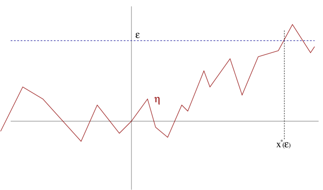
Figure 1: An illustration of the WKB method: the random landscape $\eta(x)$ starting from the value 0 at the origin $x=0$ crosses for the first time the energy level $\mathcal{E}={E}/{\sqrt{2\Gamma}}$ at the turning point $x^{*}(\mathcal{E})$.

We now estimate $n_{E}(0)$. First, we rewrite the Schrödinger equation (46) as

$$\frac{d^{2}n_{E}(x)}{dx^{2}}+\frac{\sqrt{2\Gamma}}{D}\left(\eta(x)-\mathcal{E}\right)n_{E}(x)=0\,,\qquad\mathcal{E}=\frac{E}{\sqrt{2\Gamma}}\,.$$ (50)

The Brownian landscape $\eta(x)$ starts at $\eta(x=0)=0$ and it will remain smaller than $\mathcal{E}$ up to a first crossing-point $x^{*}(\mathcal{E})>0$ such that $\eta(x^{*})=\mathcal{E}$ (see Figure 1). We know the typical scaling $x^{*}(\mathcal{E})\sim\mathcal{E}^{2}$. Because $\eta(x)$ is a non-monotonous function of $x$, there will be many subsequent crossing points. (For the Brownian landscape, there will be infinitely many crossing points immediately following the first crossing BM .) We are interested in the behavior in the vicinity of the origin, see Eq. (49), so these further crossing points play a little role.

In the long-time limit, the dominant contribution into the integral in (49) is provided by large values of ‘energy’ $E$. (We shall confirm this assertion below.) Therefore we can analyze Eq. (50) using the WKB method Migdal ; BO78 . On the interval $x<x^{*}$, the WKB solution reads

$$n_{E}(x)\sim\frac{1}{\left(\mathcal{E}-\eta(x)\right)^{1/4}}\,{\exp}\left({\frac{-(2\Gamma)^{1/4}}{\sqrt{D}}\int_{x}^{x^{*}(\mathcal{E})}}dx^{\prime}\,\sqrt{\mathcal{E}-\eta(x^{\prime})}\right)$$ (51)

We now define $x^{\prime}=\mathcal{E}^{2}\tau$ and use the scaling property $\eta(\mathcal{E}^{2}\tau)\equiv\mathcal{E}\eta(\tau)$. Then, from the expression (51), we obtain (keeping again only the dominant exponential factor)

$$n_{E}(0)\sim\exp\!\left(-\frac{{E}^{5/2}}{2\Gamma\sqrt{D}}\,\int_{0}^{\tau^{*}}d\tau\,\sqrt{B_{\tau}}\right)$$ (52)

where $\tau^{*}$ represents the first moment when the Brownian motion $B_{\tau}=1-\eta(\tau)$ that starts at 1 at $\tau=0$, crosses the origin: $B_{\tau}>0$ for $\tau<\tau^{*}$ and $B_{\tau^{*}}=0$.

We now consider a typical realization $\eta$ of the landscape. The integral that appears in (52) has a constant value $K_{\eta}$ that depends on the landscape. Thus

$$n_{E,\text{typ}}(0)\sim\exp\!\left(-K_{\eta}\frac{{E}^{5/2}}{2\Gamma\sqrt{D}}\right)\,.$$ (53)

Substituting this expression in the spectral decomposition (49) leads to

$$n_{\text{typ}}\sim\int dE\,\exp\!\left(Et-K_{\eta}\frac{{E}^{5/2}}{2\Gamma\sqrt{D}}\right)\sim\exp\!\left[\frac{3}{5}\left(\frac{4}{5K_{\eta}}\right)^{2/3}(\Gamma^{2}Dt^{5})^{1/3}\right].$$ (54)

The second asymptotic in (54) has been derived via the saddle-point method. The maximum of the integrand occurs at $E\sim t^{2/3}$ which diverges as $t\to\infty$; this justifies the use of the WKB solution (51). The final result (54) qualitatively agrees with the prediction of Eq. (39) which was established using heuristic arguments.

We now determine the value of the average population $\langle n\rangle$, where the average is taken over all possible realizations of the noise. First, we need to calculate

$$\langle n_{E}(0)\rangle\sim\left\langle\exp\!\left(-\frac{{E}^{5/2}}{2\Gamma\sqrt{D}}\,\int_{0}^{\tau^{*}}d\tau\,\sqrt{B_{\tau}}\right)\right\rangle\,,$$ (55)

where the expectation value is taken over all Brownian paths starting at 1 at $\tau=0$ and vanishing at $\tau^{*}$ for the first time. This expression is the average of a first passage exponential functional of the Brownian motion and its value can be determined using the general method described e.g. in Ref. Satya . The procedure applies to a functional of the form

$$Q(x_{0})\equiv Q(x_{0};p,\mathcal{U})=\left\langle\exp\!\left(-p\,\int_{0}^{\tau^{*}}d\tau\,{\mathcal{U}}(B_{\tau})\right)\right\rangle$$ (56)

that involves an arbitrary smooth function ${\mathcal{U}}(B_{\tau})$ replacing $\sqrt{B_{\tau}}$ which appears in (55). The normalized Brownian process starts at any $x_{0}>0$ and as a function of $x_{0}$, the functional (56) satisfies the backward Fokker-Planck equation

$$\frac{1}{2}\frac{d^{2}Q(x_{0})}{dx_{0}^{2}}-p\,{\mathcal{U}}(x_{0})Q(x_{0})=0$$ (57)

with the boundary conditions

$$Q(x_{0}=0)=1\,\,\hbox{ and }\,\,Q(x_{0}\to+\infty)=0\,.$$ (58)

Our problem, equation (55), perfectly fits into this framework. Thus we must solve the following differential equation:

$$\frac{1}{2}\frac{d^{2}Q(x_{0})}{dx_{0}^{2}}-p\sqrt{x_{0}}Q(x_{0})=0\,\,\hbox{ where }\,\,p=\frac{{E}^{5/2}}{2\Gamma\sqrt{D}}\,.$$ (59)

We need to calculate $Q(1)$ because the Brownian paths in equation (55) start at $x_{0}=1$. The asymptotic behavior of the solution of Eq. (59) can again be obtained via the WKB method. Writing $Q={\rm e}^{S}$ we find $S(x_{0})=-\tfrac{4}{5}\,\sqrt{2p}\,(x_{0})^{5/4}$ in the leading order. Therefore

$$\langle n_{E}(0)\rangle\sim\exp\!\left(-\frac{4{E}^{5/4}}{5\,\Gamma^{1/2}D^{1/4}}\right)\,.$$ (60)

Inserting this result into equation (49) and evaluating the integral by saddle-point method we arrive at

$$\langle n\rangle\sim\exp\!\left(\tfrac{1}{5}D\Gamma^{2}t^{5}\right)\,.$$ (61)

This exact asymptotic qualitatively agree with Eq. (41) which was derived using qualitative arguments.

As a side remark, we notice that the growth laws in judiciously chosen deterministic landscapes $\eta(x)$ shed light on the growth laws in random landcapes. For instance,

• If we consider $\eta(x)=\kappa x$, then equation (1) admits an exact solution

  $$n(x,t)=\frac{1}{\sqrt{4\pi Dt}}\,\,\exp\!\left(-\frac{(x-\kappa Dt^{2})^{2}}{4Dt}+\frac{\kappa^{2}Dt^{3}}{3}\right)$$

  representing a Gaussian profile with uniformly accelerated center and with total mass growing as ${\rm e}^{t^{3}}$. This solution can be obtained by the previously described spectral analysis: $n_{E}(x)={\rm Ai}(E-x)$ where ${\rm Ai}$ is the Airy function. This example can be used as a template for applying the WKB method. Note that this solution is well-known in quantum mechanics as an ‘Airy Packet’, that spreads without changing its form Berry .

• For $\eta(x)=\kappa x^{2}$, the path integral (4) is quadratic and can be calculated exactly Schulman . The solution is given by

  $$n(x,t)=\left(\frac{\kappa}{D}\right)^{1/4}\,\frac{1}{\sqrt{2\pi\sin(2\,(D\kappa)^{1/2}\,t)}}\exp\left(-\frac{\sqrt{\kappa}\,x^{2}}{2\sqrt{D}}\frac{\cos(2\,(D\kappa)^{1/2}\,t)}{\sin(2\,(D\kappa)^{1/2}\,t)}\right)\,.$$

  The total population corresponding to this solution, $N=1/\sqrt{\cos[2\,(D\kappa)^{1/2}\,t]}$, blows up at the finite time $t_{c}=\,(D\kappa)^{-1/2}\,\frac{\pi}{4}\,.$

• For $\eta(x)=\kappa\,{\rm sign}(x)|x|^{\alpha}$, with $0<\alpha<2$, the WKB analysis can be carried out again and one finds that the total population increases as

  $$N\sim\exp\!\left(\frac{2-\alpha}{2+\alpha}\left(A(\alpha)^{2\alpha}D^{\alpha}\kappa^{2}t^{2+\alpha}\right)^{\frac{1}{2-\alpha}}\right)\,,\quad A(\alpha)=\frac{2\alpha^{2}\Gamma(3/2+1/\alpha)}{(2+\alpha)\Gamma(3/2)\Gamma(1/\alpha)}\,.$$

For $\alpha=1/2$, we arrive at the $\exp(t^{5/3})$ growth that was obtained for a typical Brownian landscape. For $\alpha=1$, we recover the $\exp\left(\kappa^{2}Dt^{3}/3\right)$ growth of the linear landscape. For $0<\alpha<1$, we obtain the same behavior as for a self-affine disordered landscape with Hurst exponent $H=\alpha$.

III.3 Population Growth in High Dimensions

When the dimension of the underlying substrate exceeds one, various types of random landscapes can arise and there is no single landscape which is as natural as the Brownian landscape in $1d$. Perhaps the closest analog of the one-dimensional Brownian landscape is a random landscape that arises by taking the ‘height’ variable $\eta({\bf R})$ to be a Gaussian free field. This class of random manifolds has been widely studied (see e.g. SS and references therein). The Gaussian free field on a discrete lattice of dimension $d$ is defined by assigning the Gaussian probability to the configuration $\eta({\bf R})$:

$$\exp\left\{-\sum[\eta({\bf R}\pm{\bf e}_{\alpha})-\eta({\bf R})]^{2}\right\}\,,$$ (62)

where the sum runs over ${\bf R}\in\mathbb{Z}^{d}$ and over ${\bf e}_{\alpha}$, which are the unit vectors in the $d$ possible directions. In the continuum limit, the summation is replaced by integration, $\int(\nabla\eta)^{2}\,d{\bf R}$. Further, one has to introduce a small-scale cut-off to regularize correlation functions on short distances SS . The Gaussian free field is characterized by the following height-correlation function:

$$\langle[\eta({\bf R})-\eta({\bf 0})]^{2}\rangle \sim \ln R\,\,\,\quad{\rm for}\,d=2\,,$$ (63)

$$\langle[\eta({\bf R})-\eta({\bf 0})]^{2}\rangle \sim {\rm finite}\,\quad{\rm for}\,d>2\,.$$ (64)

One can also define random landscapes by using the Edwards-Wilkinson growth process HHZ which has the same 2-point correlation functions as above.

III.3.1 Typical Growth

We estimate the typical growth using the same argument as in one dimension, namely by balancing the typical maximal value of the noise over a radius $R$ with the probability for the particles to visit a droplet of size $R$:

$$n_{\rm typ}\sim\exp\!\left[t\sqrt{\ln R}-\frac{R^{2}}{4t}\right]\,.$$ (65)

Maximizing with respect to $R$ gives $R\sim t(\ln t)^{1/4}$ leading to

$$n_{\rm typ}\sim e^{t\sqrt{\ln t}}\,.$$ (66)

In dimensions strictly higher than 2, if we consider a random landscape generated by a Gaussian free field then the landscape is statistically flat, i.e., its width does not vary with the macroscopic length scale $R$ (it depends in fact on the microscopic cut-off). Therefore, the typical population grows exponentially.

To summarize, we have the following growth laws for the typical population under a random landscape

$$n_{{\rm typ}}\sim\begin{cases}e^{t^{5/3}}&\text{ for }d=1\\ e^{t\sqrt{\ln t}}&\text{ for }d=2\\ e^{t}&\text{ for }d\geq 3\,.\end{cases}$$ (67)

Finally, we note that random surfaces characterized by the logarithmically growing height-correlation function (63) are almost flat. One can consider random surfaces with algebraic height-correlation function (see e.g. K ) given by $\langle[\eta({\bf R})-\eta({\bf 0})]^{2}\rangle\sim R^{\zeta}.$ We then obtain $n_{\rm typ}\sim\exp\!\left[tR^{\zeta/2}-\frac{R^{2}}{4t}\right]$, from which we conclude that

$$n_{\rm typ}\sim\exp\!\left[t^{(4+\zeta)/(4-\zeta)}\right]\,.$$ (68)

III.3.2 Average Growth

The typical growth laws obtained above correspond to a given realization of the Gaussian free field $\eta({\bf R})$. The average growth of the population is again dominated by the very rare fluctuations of the landscape. To derive the average growth we need, as in one dimension, to keep two free parameters: the size $R$ of the droplet visited by the particles and the maximum value $M$ reached by $\eta({\bf R})$ over this droplet.

In two dimensions, a heuristic estimate is found by taking a Gaussian distribution for $M$ of variance $\ln R$:

$$\langle n\rangle\sim\exp\!\left[tM-\frac{M^{2}}{2\,\ln R}-\frac{R^{2}}{4t}\right]\,.$$ (69)

Maximizing with respect to $M$ and $R$, we find

$$\langle n\rangle\sim e^{t^{2}\,\ln t}\,.$$ (70)

A rigorous derivation of this estimate is perhaps a challenging problem. Nevertheless, we can justify why the distribution of the maximum value $M$ of a Gaussian free field has a Gaussian tail. Let us first revisit the $d=1$ case. The full distribution of the maximum of a Brownian process is of course well-known BM , yet we want to deduce its tail in a simple way that will admit a generalization to the Gaussian free field. The tail of the maximum distribution can be retrieved by the following simple reasoning: let us consider a Brownian path $h(x)$ of length $L$ with $h(0)=0$ and let $M$ be its maximum value; when $M$ is large, the maximum must be reached in the vicinity of the end of the path and such a path contributes by a weight of $\exp(-\tfrac{1}{2}\int(h^{\prime}(x))^{2}dx)$. The optimal path that has the largest weight is therefore obtained by minimazing the integral $\int_{0}^{L}(h^{\prime}(x))^{2}dx$. This gives $h^{\prime\prime}=0$, which in conjunction with $h(0)=0$ and $h(L)=M$, leads to $h(x)=Mx/L$. Substituting this expression in the exponential weight, we arrive at the tail $\exp(-M^{2}/2L)$ which we used in Eq. (40).

Turning to two dimensions, let us consider a Gaussian random surface $h(x,y)$ over a circular disk of radius $R$. As in $d=1$ we expect the maximum value $M$ of the height $h$ to be reached on the rim of the disk. Supposing that the optimal surface is rotationally invariant, its statistical weight is given by $\exp(-\tfrac{1}{2}\int(\frac{\partial h}{\partial r})^{2}rdr)$ in radial coordinate $r$. Optimizing this weight with the constraints $h(0)=0$ and $h(R)=M$ leads to the Euler-Lagrange equation:

$$\frac{d}{dr}\left(r\frac{dh}{dr}\right)=0\,.$$

The solution to this equation is $h(r)=M\frac{\ln r}{\ln R}$ and the weight of this optimal path is given by

$$\exp\left(-\frac{M^{2}}{2(\ln R)^{2}}\int_{1}^{R}\frac{dr}{r}\right)=\exp\left(-\frac{M^{2}}{2\ln R}\right)\,,$$

where a short-length scale cut-off (we set it to unity) allows to avoid the small $r$ divergence. This justifies the expression of the distribution of $M$ used in equation (69).

Growth in various $d$	Typical	Average
One dimension	$e^{t^{5/3}}$	$e^{t^{5}}$
Two dimensions	$e^{t\sqrt{\ln t}}$	$e^{t^{2}\ln t}$
Higher dimensions ($d>2$)	$e^{t}$	$e^{t^{2}}$

Table 2: Asymptotic growth laws in a Gaussian random landscape. In order to regularize short scale fluctuations in $d\geq 2$, the Gaussian free field is defined on a lattice. For $d=1$, the results were already given in Table 1.

A similar reasoning can be carried out in higher dimensions. In order to estimate the average growth we again need to know the distribution of the maximum. Proceeding as above we find that in three dimensions, the spherically symmetric optimal landscape satisfies $\frac{d}{dr}\left(r^{2}\frac{dh}{dr}\right)=0$ with respect to the radial coordinate $r$. This leads to $h(r)=M\frac{R(r-1)}{r(R-1)}\to M\big{(}1-r^{-1}\big{)}$ (taking again the microscopic cut-off to be unity). The corresponding weight behaves as $\exp(-M^{2}/2)$; there is no dependence on $R$ because the interface is flat at large scales. Using this expression for the maximum distribution, we obtain the average growth of the population

$$\langle n\rangle\sim\exp\!\left[tM-\frac{M^{2}}{2}-\frac{R^{2}}{4t}\right]\,.$$

in three dimensions. Maximizing with respect to $M$ we arrive at

$$\langle n\rangle\sim e^{t^{2}}\,.$$ (71)

Note that we do not need to optimize with respect to $R$ because the distribution of $M$, for large values of $M$, is independent of $R$. A similar reasoning can be carried out in higher dimensions and we find that the behavior is also given by (71) for all $d>2$.

Table 2 summarizes our results for the typical and the average population growth in the situation when the random landscape is described by a Gaussian free field.

IV Conclusion

In this work, we have investigated the evolution of a population of non-interacting particles that undergo diffusion and birth/death. The latter depends on the environment, for example, the distribution of nutrients that defines a landscape which is assumed to be stationary. Different statistical properties of this landscape lead to a number of laws for the growth of the population. In most of the cases, the total population increases in a faster-than-exponential manner. This behavior is due to two features of the noise, namely its multiplicative nature and the lack of upper bound. Another striking feature is the huge difference between typical and average behaviors. In order to determine the average growth law, one has to consider all possible realizations of the random landscape and the average is dominated by very rare configurations. Thus extremal statistics play an important role. Some of our analysis relies on heuristic arguments. In one dimension we have performed asymptotically exact calculations in the situation where the noise is described by a Brownian process. We have shown that the determination of the average population growth reduces to calculating a first passage exponential functional of the Brownian motion. This problem can be solved by using the Backward Fokker-Planck equation. The asymptotically exact results agree with heuristic predictions.

Although the basic stochastic differential equation (1) has been studied for almost thirty years, there are still many open problems. Even in one dimension, it would be interesting to generalize the quantitative approach applicable to the Brownian landscape to other random landscapes such as those generated by a fractional Brownian motion. In higher dimensions ($d\geq 2$), little is rigorously and/or exactly known. To appreciate the challenge, one can think of the somewhat related problem of the localization of a quantum particle.

On a more practical side, it could be interesting to study the transient regime when the system is still far from the final asymptotic stage. In the long time limit, non-linear saturation effects, that are ignored in our model, can start playing a prominent role. Adding nonlinear terms to the basic equation (1) will totally modify its properties in the asymptotic regime. This is a challenging mathematical problem that deserves further analysis.

The work of PLK has been supported by NSF Grant No. CCF-0829541. We are thankful to M. Bauer, F. David, B. Duplantier, S. Mallick, and S. Redner for suggestions, help, and encouragement.

References

- (1) Y. B. Zeldovich, S. A. Molchanov, A. A. Ruzmaikin and D. D. Sokolov, Zh. Eksp. Teor. Fiz. 89, 2061 (1985) [Sov. Phys. JETP 62, 1188 (1985)].
- (2) M. B. Isichenko, Rev. Mod. Phys. 64, 961–1043 (1992).
- (3) Y. B. Zeldovich, S. A. Molchanov, A. A. Ruzmaikin and D. D. Sokolov, Usp. Fiz. Nauk. 152, 3 (1987) [Sov. Phys. Usp. 30, 353 (1987)].
- (4) J. D. Murray, Mathematical Biology (Springer-Verlag, New-York, 1993).
- (5) W. J. Ewens, Mathematical Population Genetics (Springer-Verlag, New York, 2004).
- (6) E. O. Budrene and H. Berg, Nature 376, 49 (1995).
- (7) M. Eigen, Naturwiss. 58, 465 (1971); M. Eigen and P. Schuster, The Hypercycle: A Principle of Natural Self-Organization (Berlin: Springer-Verlag, 1979).
- (8) W. Ebeling, A. Engel, B. Esser and R. Feistel, J. Stat. Phys. 37, 369 (1984); A. Engel and W. Ebeling, Phys. Rev. Lett. 59, 1979 (1987).
- (9) Y. C. Zhang, Phys. Rev. Lett. 56, 2113 (1986).
- (10) M. N. Rosenbluth, Phys. Rev. Lett. 63, 467 (1989).
- (11) E. Baake and W. Gabriel, “Biological evolution through mutation, selection, and drift: An introductory review.” In D. Stauffer (Ed.), Annual Reviews of Computational Physics VII, pp. 203–264 (2000).
- (12) K. Jain and J. Krug, “Adaptation in simple and complex fitness landscapes.” In U. Bastolla, M. Porto, H. Roman, and M. Vendruscolo (Eds.), Structural approaches to sequence evolution: Molecules, networks and populations (Berlin: Springer, 2006).
- (13) D. R. Nelson and N. M. Shnerb, Phys. Rev. E 58, 1383 (1998).
- (14) K. A. Dahmen, D. R. Nelson and N. M. Shnerb, J. Math. Biol. 41, 1 (2000).
- (15) M. M. Desai and D. R. Nelson, Theor. Popul. Biol. 67, 33 (2005).
- (16) N. M. Shnerb, E. Bettelheim, Y. Louzoun, O. Agam and S. Solomon, Phys. Rev. E 63, 21103 (2001).
- (17) Y. Tsoti and P.-G. de Gennes, Europhys. Lett. 66, 599 (2004); P.-G. de Gennes, Eur. Biophys. J. 33, 691 (2004).
- (18) A. Celani and M. Vergassola, Proc. Natl. Acad. Sci. 107, 1391 (2010).
- (19) Y. B. Zeldovich, S. A. Molchanov, A. A. Ruzmaikin and D. D. Sokolov, Proc. Natl. Acad. Sci. 84, 6323 (1987).
- (20) A. S. Mikhailov and I. V. Uporov, Usp. Fiz. Nauk. 144, 79 (1984) [Sov. Phys. Usp. 27, 695 (1984)].
- (21) A. S. Mikhailov, Phys. Rep. 184, 307 (1989).
- (22) M. D. Donsker and S. R. S. Varadhan, Comm. Math. Phys. 28, 525 (1975).
- (23) B. Ya. Balagurov amd V. G. Vaks, Zh. Eksp. Teor. Fiz. 65, 1939 (1973) [Sov. Phys. JETP 38, 968 (1974)].
- (24) P. Grassberger and I. Procaccia, J. Chem. Phys. 77, 6281 (1982).
- (25) S. Redner and K. Kang, Phys. Rev. A 30, 3362 (1984).
- (26) J. K. Anlauf, Phys. Rev. Lett. 52, 1845 (1984).
- (27) T. M. Nieuwenhuizen, Phys. Rev. Lett. 62, 357 (1989).
- (28) J.-M. Luck and T. M. Nieuwenhuizen, J. Stat. Phys. 52, 1 (1988).
- (29) J.-M. Luck, Systèmes Désordonnés Unidimensionnels (Alea-Saclay, 1992).
- (30) L. S. Schulman, Techniques and Applications of Path Integration (Dover, New-York 2005).
- (31) D. A. Huse and C. L. Henley, Phys. Rev. Lett. 54, 2708 (1985).
- (32) S. F. Edwards and M. Muthukumar, J. Chem. Phys. 89, 2435 (1988).
- (33) M. E. Cates and R. C. Ball, J. Phys. France 59, 2009 (1988).
- (34) T. Nattermann and W. Renz, Phys. Rev. A 40, 4675 (1989).
- (35) J. Krug and T. Halpin-Healy, J. Phys. France 3, 2179 (1993).
- (36) T. Halpin-Healy and Y. C. Zhang, Phys. Rep. 254, 215 (1995).
- (37) M. Kardar, G. Parisi and Y. C. Zhang, Phys. Rev. Lett. 56, 889 (1986).
- (38) I. M. Lifshitz, S. A. Gredeskul and L. A. Pastur, Introduction to the Theory of Disordered Systems (New-York, Wiley, 1988).
- (39) R. A. Guyer and J. Machta, Phys. Rev. Lett. 64, 494 (1990); J. Machta and R. A. Guyer, J. Phys. A 22, 2539 (1989).
- (40) H. Leshke and S. Wonneberger, J. Phys. A 22, L1009 (1989).
- (41) R. Tao, Phys. Rev. Lett. 61, 2405 (1988); 63, 2695 (1989).
- (42) R. Tao, Phys. Rev. A 43, 5284 (1991).
- (43) A. M. Jayannavar and J. Köhler, Phys. Rev. A 41, 3391 (1990).
- (44) E. P. Gross, J. Stat. Phys. 33, 107 (1983).
- (45) P. L. Krapivsky, S. Redner and E. Ben-Naim, A Kinetic View of Statistical Physics (Cambridge: Cambridge University Press, 2010).
- (46) F. A. B. F. de Moura and M. L. Lyra, Phys. Rev. Lett. 81, 3735 (1998).
- (47) J. W. Kantelhardt, S. Russ, A. Bunde, S. Havlin and I. Webman, Phys. Rev. Lett. 84, 198 (2000).
- (48) J.-M. Luck, J. Phys. A: Math. Gen. 38, 987 (2005).
- (49) P. Mörders and Y. Peres, Brownian Motion (Cambridge: Cambridge University Press, 2010).
- (50) A. B. Migdal, Qualitative Methods in Quantum Theory (W. A. Benjamin, Inc. 1977).
- (51) C. M. Bender and S. A. Orszag, Advanced Mathematical Methods for Scientists and Engineers (McGraw-Hill, New York, 1978).
- (52) S. N. Majumdar, Curr. Science, 89, 2077 (2007).
- (53) M. V. Berry and N. L. Balazs, Am. J. Phys. 47, 264 (1979).
- (54) O. Schramm and S. Sheffield, Acta Math. 202, 21–137 (2009).
- (55) J. Kondev, C. L. Henley, and D. G. Salinas, Phys. Rev. E 61, 104 (2000).